SCUOLA DI SCIENZE
Corso di Laurea Magistrale in Informatica
REINFORCEMENT LEARNING
IN ROGUE
Relatore:
Chiar.mo Prof.
ANDREA ASPERTI
Presentata da:
DANIELE CORTESI
Sessione I
Anno Accademico 2018/2019
Reinforcement learning (RL) is a machine learning framework that in-volves learning to interact with an environment in such a way that maxi-mizes a numerical reward signal, without human supervision. This is po-tentially better than developing hard-coded programs that interact with the environment, due to the thorough knowledge of its mechanisms that the lat-ter approach requires. No such understanding is needed in RL, that can nonetheless produce surprisingly good policies exclusively by trial-and-error, although it can certainly be included when available. Moreover, RL has been able to devise better and novel strategies than those previously known: e.g. in the game of Backgammon [44] it learned unprecedented opening moves good enough to be adopted by professional players. In problems encompassing large state spaces — i.e. exhibiting an intractable amount of configurations, like Backgammon or Chess board positions — some approximation method is fundamental. Neural networks (see section 1.2.3) are powerful nonlinear function approximators inspired to biological brains that are often preferred for this task and we will be the basis of our work.
Recently RL has attracted a lot of attention due to the results attained by Mnih et al. [29] in Atari 2600 games. The authors developed a novel Q-learning algorithm and had a neural network, that they call deep Q-network (DQN), learn to play with fixed hyper-parameters the games available on the platform from almost raw pixels and using only the score as a reward, achieving expert human level play on many of them and super human levels on several others. This break through inspired a considerable amount of
deavors, summarized in [26], that improved on the results either by enhancing DQN or by entirely different approaches.
This work aims at automatically learning to play, by RL and neural net-works, the famous Rogue, a milestone in videogame history that we describe throughly in chapter 2. It introduced several mechanics at its core, spawning the entire rogue-like genre, like procedural (i.e. random) level generation, permadeath (i.e. no level replay) and other aspects discussed in section 2.2, that make it very challenging for a human and constitute an interesting RL benchmark. Related works on this game started with Pedrini’s thesis [34], to which our own can be considered a spiritual successor, and continued with [3, 4]. Several problems emerged there that we successfully addressed here, enabling us to obtain much better results and investigate new scenarios where we encountered further obstacles. Games are possibly the most popular test-ing ground for RL methods, because they are designed to challenge human skills and are often simplified simulations of reality. Many environments exist for training RL agents to play games, such as [6, 8] for arcade games, [8] for some continuous control tasks, [22] for the famous DOOM and very recently [46] for StarCraft II (please see section 1.3 for more details and other RL applications). Rogueinabox [34, 3] is the sole environment for Rogue we are aware of, see section 2.3 for more details and rogue-like environments.
In the following, we introduce the RL theoretical background in chapter 1 and then present Rogue in chapter 2. We proceed to discuss our experiments in chapter 3 and then draw the conclusions.
Introduction i 1 Reinforcement Learning 3 1.1 Elements of RL . . . 4 1.1.1 Agent . . . 4 1.1.2 Environment . . . 5 1.1.3 Model . . . 6 1.1.4 Policy . . . 7 1.1.5 Reward signal . . . 7 1.1.6 Value function . . . 7
1.1.7 Optimal policy and value functions . . . 8
1.2 RL algorithms . . . 10
1.2.1 On-policy vs Off-policy . . . 10
1.2.2 Bootstrapping and temporal-difference learning . . . . 11
1.2.3 Function approximation and neural networks . . . 12
1.2.4 The Deadly Triad . . . 15
1.2.5 Q-learning and DQN . . . 15
1.2.6 Policy gradient and REINFORCE . . . 16
1.2.7 Actor-Critic and A3C . . . 19
1.2.8 ACER . . . 21
1.3 RL applications . . . 25
2 Rogue 27 2.1 A game from the 80ies . . . 28
2.2 A difficult RL problem . . . 28
2.3 Rogueinabox . . . 31
3 Learning to play Rogue 33 3.1 Problem simplification . . . 33
3.2 Objectives . . . 34
3.3 Descending the first level . . . 35
3.3.1 Evaluation criteria . . . 35
3.3.2 Partitioned A3C with cropped view . . . 36
3.3.3 Towers with A3C and ACER . . . 46
3.4 Descending until the tenth level . . . 57
3.4.1 Evaluation criteria . . . 58
3.4.2 Towers with ACER . . . 58
3.5 Recovering the amulet from early levels . . . 64
3.5.1 Evaluation criteria . . . 65
3.5.2 First level . . . 66
3.5.3 Second level . . . 67
Conclusions 71 A ACER code 73 A.1 Main loop . . . 73
A.2 Environment interaction and training . . . 74
B Three towers analysis 77
1.1 Markov Decision Process dynamics . . . 5
1.2 Neural network legend . . . 14
1.3 A3C neural network . . . 20
2.1 A Rogue screenshot . . . 27
3.1 Neural network architecture for partitioned A3C . . . 38
3.2 Results of partitioned A3C with cropped view . . . 44
3.3 Three towers neural network architecture for ACER . . . 50
3.4 Results of A3C and ACER without situations . . . 55
3.5 Best results on the first level comparison . . . 56
3.6 Dark rooms and labyrinths . . . 59
3.7 Results of ACER until the 10th level . . . 60
3.8 Dark rooms and labyrinths statistics . . . 63
3.9 Results of recovering the amulet from the first level . . . 66
3.10 ACER agent struggling . . . 68
3.11 Results of recovering the amulet from the second level . . . 69
B.1 Three towers focus . . . 79
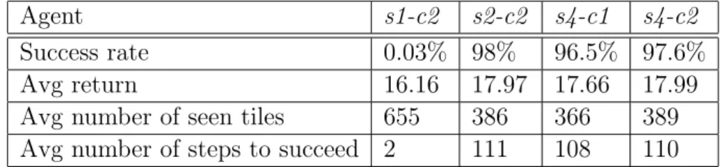
3.1 Hyper-parameters for partitioned A3C with cropped view . . . 43
3.2 Partitioned A3C with cropped view final results . . . 43
3.3 Hyper-parameters for ACER . . . 54
3.4 Final results of A3C and ACER without situations . . . 55
3.5 Final results of ACER descending until the tenth level . . . . 61
3.6 Dark rooms and labyrinths statistics . . . 62
3.7 Results until the tenth level with more steps . . . 64
3.8 Results of recovering the amulet from the first level . . . 67
3.9 Results of recovering the amulet from the second level . . . 68
Reinforcement Learning
Reinforcement learning (RL) is a machine learning setting involving an agent interacting with an environment that changes in relation to the actions performed. The agent receives a numerical reward signal for each action taken and seeks to maximize the cumulative reward obtained in the long run, despite the uncertainty about the environment. Since actions affect the opportunities available at later times, the correct choices require taking into account their indirect and delayed consequences, which may require foresight or planning. The RL framework is an abstraction of the problem of goal-directed learning from interaction, in which all relevant details are reduced to the environment states, the actions performed and the rewards consequently received, which define the goal of the problem. RL is strongly linked with psychology and neuroscience: of all forms of machine learning, it is the closest to the way that humans and other animals learn [41].
The main characteristics of RL are:
• being a closed-loop problem, such that the actions taken influence the later inputs, available actions and rewards;
• not having direct instructions as to what actions to take;
• the consequences of actions, and subsequent rewards, play out over extended periods of time.
RL differs from supervised learning in that there is no set of labeled ex-amples provided by an external supervisor. In essence, it uses training infor-mation that evaluates its actions rather than instructing them by providing correct samples. Such feedback indicates how good the action taken is, but not whether it’s the best or worst one possible. It would also be impractical to form a set of such examples that is both correct and representative of all the situations in which the agent is expected to act optimally. Moreover, RL is renown for producing optimal behaviors that were previously unknown, such as in the games of Backgammon [44] and Go [38, 39].
RL is also different from unsupervised learning, as it tries to maximize a reward signal instead of uncovering a hidden structure in unlabeled data.
To make the distinction even clearer, there is an important issue that arises only in RL: the trade-off between exploration and exploitation. An agent must in fact prefer actions it has tried in the past that were found to be effective in producing reward, however to discover such actions it has to try ones it has not selected before. The point is that neither exploration nor exploitation alone are sufficient to succeed at the task: they must be combined, typically by progressively shifting the focus from exploration to exploitation.
1.1
Elements of RL
In this section we present the main elements of the RL framework.
1.1.1
Agent
The entity continually interacting with the environment. The first selects actions according to a policy and the the second responds by presenting new observations and rewards. The agent can either be a complete organism or a component of a larger system. The boundary between the agent and the environment is usually drawn very close to the agent: for example, if it has arms then they are considered part of the environment and in general so
is everything that cannot be arbitrarily changed by the agent. The agent-environment boundary represents the limit of the agent’s absolute control, but not of its knowledge, in fact it may know to any degree how the rewards are computed as a function of its actions.
1.1.2
Environment
In general a Partially Observable Markov Decision Process (POMDP) [33, 30]. Formally, a MDP is a tuple (S, A, p), where:
• S is the set of possible states;
• A is the set of possible actions, with A(st) denoting the actions available
at time t in state st∈ S;
• p : S ×R×S ×A → [0, 1] is the probability function of state transitions, such that p(s, r|st, at) denotes the probability of a next state-reward
pair following a a state-action pair at time t. Often p(s|st, at) is used
to denote the probability of transitioning to state s without considering a specific reward. --- --- --- |...| |...+###### |...| |...+######### |...| ###+.!....| |...| ##############+...| -+--- ---+- ---+- # # # # ######### # #### # ---+---- # # |...| -+--- ---+- |...| |...| |.*...| |...| |...*.| |...%..@...| |...| |...| ---+--- ---+--- |...!...| # -+--- # # ######## ##### # -+--- --+-- |...| |...+##################+...?| |...| |...| |...| --- --- Level: 1 Gold: 3 Hp: 12(12) Str: 16(16) Arm: 4 Exp: 1/0 Cmd: 265
Environment
a
s
s
Agent
r
Figure 1.1: Markov Decision Process dynamics
The interaction between the agent and the environment is divided in discrete time steps t = 0, 1, 2, . . . At each time step the agent receives a representation of the environment state st ∈ S, selects an action at ∈ A(st)
according to a policy π and then receives the next state and reward st+1, rt
sampled from p(·, ·|st, at). We define a state-action trajectory the sequence
st, at, st+1, at+1, . . . , sT of states observed and actions taken from time t to
T . The steps are not required to refer to fixed intervals of time and likewise the actions may be low or high level controls, such as motor voltages or the decision of a destination, respectively. We will solely consider the episodic case in which the interaction with the environment naturally breaks down in episodes, i.e. in many independent finite trajectories ending in a final state. The opposite case, called continuing case, is also studied and described in [41].
Most of RL theory is developed assuming the Markov Property, an at-tribute that the states presented by the environment have if they contain all relevant information for predicting future states, e.g. the position of all pieces in a chess game. The algorithms are nonetheless successfully applied often times even in its absence: people can make very good decisions in non-Markov tasks, e.g. poker, so arguably this should not be a severe problem for a RL agent.
1.1.3
Model
A system that is able to predict how the environment will behave. It can be used for planning, i.e. deciding the sequence of future actions considering possible future situations before they are actually experienced. Methods for solving RL problems that use models and planning are called model-based, while simpler methods that are exclusively trial-and-error learners are referred to as model-free. The latter are much more effective than they may appear, which makes RL very powerful indeed: complex sequences of actions that maximize the future cumulative reward received can be learned without any prior knowledge of the environment dynamics. In this work will focus on model-free approaches and will not discuss the model-based alternative, which is explained in [41].
1.1.4
Policy
The definition of the agent’s way of behaving at a given time. It is a map-ping, or a probability distribution, from perceived states of the environment to actions to be taken. Formally, a policy is a function π : A × S → [0, 1] and the probability of selecting action a in state st at time step t is denoted
πt(a|st).
1.1.5
Reward signal
The definition of the goal in a RL problem. On each time step, the envi-ronment sends the agent a number representing the reward. The objective of the learning agent is to maximize the total reward received in the long run. Importantly the process generating the reward must be unalterable by the agent and its definition should be devised with care: we must reward only what we want the agent to achieve, but not how to achieve it. If subgoals are rewarded, e.g. taking enemy pieces in a chess game, the agent might learn just to accomplish such subgoals instead of what we really want to achieve, e.g. winning the chess game.
1.1.6
Value function
The total amount of reward the agent can expect to accumulate over the future, starting from a given state. This represents an indication of the long-term desirability of states, e.g. one may yield a low immediate reward but be regularly followed by states that yield high rewards, or the opposite. More formally, the value function corresponds to the expected return of a state s. The return is defined as Gt=
∑T
k=0γkrt+k where T is the final time step and
γ ∈ [0, 1] is a discount factor, which regulates how strongly future rewards
are taken into consideration. Hence a value function is defined as:
which denotes the expected return of starting in s and then following the policy π. This is called state-value function for policy π. The learning agent should seek actions that bring about states of highest value and not highest reward, because these are the actions that will obtain the greatest amount of reward over the long run. Values must be estimated and re-estimated from the sequences of observations an agent makes over its entire lifetime: as such a method for efficiently estimating values is crucial.
Another important function is qπ, the action-value function, which is
defined as:
qπ(s, a) =Eπ[Gt|st = s, at= a] (1.2)
The q and v functions are related in the following way: vπ(s) = ∑ a π(a|s)qπ(s, a) (1.3) q(s, a) =∑ s′,r p(s′, r|s, a)[r + γvπ(s′)] (1.4)
State value functions satisfy a recursive relationship, known as the Bell-man equation: vπ(s) =Eπ[Gt|st= s] =Eπ[rt+ γGt+1|st = s] =∑ a π(a|s)∑ s′,r p(s′, r|s, a)[r + γEπ[Gt+1|st+1 = s′]] =∑ a π(a|s)∑ s′,r p(s′, r|s, a)[r + γvπ(s′)], ∀s ∈ S (1.5)
An analogous equation can be derived for action value functions. This rule forms the basis of many ways to approximate vπ via update or backup
oper-ations, that transfer value information back to a state from its successors, or to state-action pairs from subsequent pairs.
1.1.7
Optimal policy and value functions
A policy π is defined to be better than or equal to another policy π′, i.e. π ≥ π′, if and only if vπ(s) ≥ vπ′(s) ∀s ∈ S. A policy that is better or equal
to all other policies is defined to be an optimal policy and is denoted by π∗. All optimal policies have the same optimal state and action value functions, defined as: v∗(s) = maxπvπ(s) and q∗(s, a) = maxπqπ(s, a). These equations
can also be written without referencing any policy, in a form known as the Bellman optimality equations:
v∗(s) = max a E[Gt|st= s, at= a] = max a E[rt+ γGt+1|st= s, at= a] = max a E[rt+ γv∗(st+1)|st = s, at= a] = max a ∑ s′,r p(s′, r|s, a)[r + γv∗(s′)] (1.6) q∗(s, a) =∑ s′,r p(s′, r|s, a)[r + γ max a′ q∗(s ′, a′)] (1.7) Once we have q∗ it’s easy to formulate an optimal policy: simply taking one of the actions that maximizes q∗(s,·) will do. In literature, those actions are called greedy actions and the policy is referred to as a greedy policy. Greedy does not imply optimal in general, however since q∗ is the estimate of the future return, and not of the future one-step reward, then a greedy policy always selects the action that maximizes the expected cumulative reward.
Using exclusively v∗ requires complete knowledge of the environment’s dynamics, i.e. p(s′, r|s, a), that would in principle allow to solve v∗ (and also q∗). However having this kind of information is rare and usually the state space of the problem is so large, e.g. in chess, that it would require thousand of years. This is actually what the value iteration [41] algorithm does: the procedure is divided in iterations, each of which computes a more precise estimate of v∗ by a formula directly derived from equation (1.6).
In practice, q∗ or v∗ are often estimated with increasing precision during the interaction with the environment, using the gathered experience. This kind of learning is usually referred to as on-line learning. Moreover, an optimal policy may not even require that the value of all states or state-action pairs be estimated, only the frstate-action that is frequently encountered.
In order to maintain a balance between exploration and exploitation in on-line learning, an ϵ-greedy policy is often used: such a policy selects the greedy action with respect to the current estimation of q∗ or v∗ with probability 1−ϵ and a random action otherwise. When greedy actions are chosen, then we are exploiting our current knowledge of the environment, otherwise we are exploring.
1.2
RL algorithms
In this sections we will describe some the most well known RL algorithms. Some of them can framed in a generalized policy iteration (GPI) scheme, while others in the policy gradient framework.
In GPI the processes of policy evaluation and improvement are alternated. The policy evaluation process computes vπ, or more generally brings its
esti-mate at a given time closer to its true value. The policy improvement process makes the current policy π greedy with respect to the updated estimate of vπ.
The two processes pull in opposing directions, because policy improvement makes the value function incorrect for the new policy, while policy evalua-tion causes π to no longer be greedy. Their interacevalua-tion however results in the convergence to optimality.
In policy gradient methods, the mapping π is learned directly via some
gradient ascent technique onE[Gt]. This has some advantages over GPI that
we discuss in section 1.2.6.
1.2.1
On-policy vs Off-policy
Algorithms are said to be on-policy if they improve the same policy that is used to interact with the environment, and off-policy if the policy improved, called target policy is different than the one used to make decisions, called behavior policy, which generates the training data and may be arbitrary in general. In both cases, the policy used for the interaction is required to take all actions with a probability strictly higher than zero and thereby is often
ϵ-greedy. In fact, exploration can only stop in the limit of an infinite number of actions in order to be sure there are no actions that are actually better than those favored at a given time. On-policy learning produce policies that are only near-optimal, because they can never stop exploring. Off-policy learning is more powerful and includes on-policy methods as a special case, but it usually suffers from greater variance and is slower to converge.
Importance sampling
Off-policy methods usually make use of importance sampling, a technique for estimating expected values under one distribution given samples from another, which is used to weights the returns according to the relative prob-ability of their trajectories occurring under the target and behavior policies, called importance-sampling ratio. The probability of a state-action trajectory st, at, st+1, at+1, . . . , sT occurring under policy π is
∏T−1
k=t π(ak|sk)p(sk+1|sk, ak).
Let µ be the behavior policy, then the importance-sampling ratio is:
ρt:T−1 = ∏T−1 k=t π(ak|sk)p(sk+1|sk, ak) ∏T−1 k=t µ(ak|sk)p(sk+1|sk, ak) = T∏−1 k=t π(ak|sk) µ(ak|sk) (1.8)
which has the interesting property of being independent of the environment dynamics. We also define ρt= ρt:t= π(aµ(att|s|stt)).
Importance sampling is necessary to compute an estimate of vπ that is
correct in relation to the policy π and unbiased, however it can be the source of high variance, because the product in (1.8) is potentially unbounded.
1.2.2
Bootstrapping and temporal-difference learning
A RL algorithm is said to bootstrap if the updates it makes are based on estimates. This kind of update is at the heart of temporal-difference (TD) learning, a technique for estimating state or action value functions. The target for the update of the simplest TD method, called TD(0) or one-step
to a policy at a given time. The complete TD(0) update is:
V (st)← V (st) + α[rt+ γV (st+1)− V (st)] (1.9)
where α∈ [0, 1] is called step-size parameter that controls the rate of learning and the starting value of V is arbitrary. The difference δt= rt+ γV (st+1)−
V (st) is called the TD error and arises in various forms throughout RL. This
form of TD evaluates every state s ∈ S and we refer to it as the tabular case. Since the target of the update involves the estimate of V , we say that TD(0) bootstraps and that it is biased. This bias is often beneficial, reducing variance and accelerating learning. The bootstrapping of one step TD methods enables learning to be fully on-line and incremental, since each update only requires a single environment transition.
The generalization of one-step TD is called n-step TD learning, and is based on the next n rewards and the estimated value of the state n steps later. The update rule thus involves n-step returns, defined as:
Gt:t+n = n−1
∑
k=0
γkrt+k+ γnVt+n−1(st+n) (1.10)
After n steps are made, the n-step TD update rule can be applied:
Vt+n(st)← Vt+n−1(st) + α[Gt:t+n− Vt+n(st)] (1.11)
The value of n that results in faster learning in practice depends on the problem and involves a trade-off: higher values of n allows a single update to take into account more future actions, at the cost of performing the first n without actually learning anything.
1.2.3
Function approximation and neural networks
In real world problems, we cannot hope to store a value for every single state in the state space, as is required by tabular methods. This is because state sets sizes are often exponential in the space required to represent a single state, which is the case for the game we want to focus on, Rogue.
In these cases we must to resort to function approximation, a scalable way of generalizing from spaces much larger than computational resources. The tools of choice for function approximation are artificial neural networks, par-ticularly deep convolutional neural networks, that are behind many of the recent successes in numerous fields of machine learning, especially computer vision [40, 42] and RL [29, 35, 28, 47]
Neural networks (NNs) are one of the most used methods of nonlinear function approximation. NNs are networks of interconnected units, the neu-rons, inspired to biological nervous systems. To each interconnection is as-sociated a real number: together these are the trainable parameters of NNs and are often called weights. The neurons are logically divided in layers, con-nected to those immediately preceding and following. The first layer is called input layer, the last output layer and in between there can be an arbitrary number of hidden layers: if these are present, the NN is referred to as a Deep Neural Network (DNN).
The most used layers are:
Dense or Fully Connected (FC) computes xi,j = σ(
∑
kWj,kxi−1,k) where
xi,j denotes the output of the j-th neuron of the i-th layer and W its
associated weight matrix. The function σ is the component that in-troduces nonlinearity in NNs: usually a rectified linear unit (ReLU) is preferred [32], defined as σ(x) = max{0, x}. The number of parameters of this kind of layer equals to input dimension times output dimension, so care should be taken when used on large inputs.
Convolution employs one or several windows, also called filters, that scan the input by moving the window on top of it, producing an output for each location. The window is moved according to stride values and its weights, referred to as kernel, are very low in quantity: only the size of kernel times the number of filters. Convolutions are known to be very powerful feature extractors and are especially good at 2-dimensional image processing, where they can learn to identify characteristics such as edges or other very localized patterns.
Recurrent layers are made of units that, in addition to the input from the preceding layer, also receive their own output at the previous step, called internal state. Via a built-in learned mechanism that combines the two, the units may “forget” (part of) the internal state and consider to a certain degree the input. Recurrent layers can thus be considered a form of learned memory of past inputs. The Long-Short Term Memory (LSTM) [18] was developed specifically to deal with the vanishing gra-dient problem [17], which is a real issue with a naive implementation of a recurrent network, because due to the chain-rule the gradient might involve a large number of factors close to zero multiplied together.
In this work we will describe several network architectures mainly by using images: refer to the legend in figure 1.2 for the meaning of each component.
C HxW,SHxSW@F (activation) M HxW,SHxSW GM LSTM N FC N (activation)
Convolution with a HxW kernel, SHxSW strides and F filters. Optionally it is followed by an activation function specified below.
Max-pooling with a HxW kernel and SHxSW strides.
Global max-pooling, equivalent to a max-pooling with a kernel of HxW equal to its input dimensions.
LSTM with N units.
Fully-connected (or dense) layer with N units, optionally followed by an activation function specified below.
1.2.4
The Deadly Triad
We face an important issue however if we combine function approxima-tion, bootstrapping and off-policy training, known as the deadly triad [41]. The combination produces a well known danger of instability and divergence, due to the following factors: the sequence of observed states presents cor-relations, small updates in (action-)value function estimate may result in a significant change in the policy and thereby alter the data distribution (because an update could change which action maximizes the function es-timate), and finally (action-)values and target values are correlated due to bootstrapping. The deadly triad was successfully addressed in [29], although only empirically without any theoretical guarantee, paving the way to a fair amount of work, summarized in [26].
1.2.5
Q-learning and DQN
Q-learning [49, 48] is an off-policy GPI TD method for estimating Q≈ q∗
demonstrated to converge to the optimal solution, at least in the tabular case, so long as all actions are repeatedly sampled in all states and the action-values are represented discretely, constituting one of the early breakthroughs in RL. We present tabular one-step Q-learning in Algorithm 1. Since the interaction with the environment is carried out by an ϵ-greedy policy on Q and its update rule actually evaluates a completely greedy policy, the algorithm classifies as off-policy.
A more recent breakthrough was achieved with Deep Q-Networks (DQNs) in [29], combining Q-learning with nonlinear function approximation and dealing with the deadly triad issue (section 1.2.4). In that work, deep convo-lutional neural networks were used to approximate the optimal action-value function q∗ and play several Atari 2600 games on the Arcade Learning Envi-ronment (ALE) [6] directly from (almost) raw pixels, in many cases reaching and surpassing expert human level scores. The results were very remarkable because no game-specific prior knowledge was involved beyond the
prepro-cessing of frames (that only consists in converting colors to luminance val-ues, stacking the last 4 frames due to artifacts of the old Atari platform and down-scaling them to save computational resources) and the very same set of parameters was used across all games. The main elements that enabled the success, addressing the instability issues, were experience replay and periodic updates of target values. Experience replay is a biologically inspired mecha-nism in which a number of state-action transitions (st, at, rt, s′t+1) are stored
and sampled for training, randomizing over the data hence reducing corre-lations in the observation sequence and smoothing over changes in the data distribution. The periodic update of target values, opposed to an immediate one, is implemented by using two separate parameter (or weight) vectors θi
and θ−i . The two vectors represent, respectively, the DQN parameters used to select actions and those used to compute the target at iteration i. The target parameters θ−i are only updated with θi every C steps, adding a
de-lay that reduces correlation with the targets and making divergence more unlikely. The authors also found that clipping the TD error term to be in
[−1, 1] further improved the stability of the algorithm. Pseudo-code is shown
in Algorithm 2.
The results of DQN were improved in [35] by prioritizing experience re-play, so that important experience transitions could be replayed more fre-quently, thereby learning more efficiently. The importance of experience transitions were measured by TD errors, such that these were proportional to the probability of being inserted in the experience memory buffer. The authors also made use of importance sampling to avoid the bias in the update distribution.
1.2.6
Policy gradient and REINFORCE
We turn now the attention to methods that directly learn a parametrized policy without consulting (action-)value functions, called policy gradient
meth-ods. As with DQN, we will denote the parameters with θ and write π(a|s; θ)
Algorithm 1 Tabular one-step Q-learning pseudo-code, adapted from [41]
1: initialize Q arbitrarily and Q(terminal-state,·) = 0
2: for each episode do
3: initialize state s
4: for each step of episode, state s is not terminal do
5: a ← action derived from Q(s, ·) (e.g. ϵ-greedy)
6: take action a, observe r, s′
7: Q(s, a) ← Q(s, a) + α[r + γ maxa′Q(s′, a′)− Q(s, a)]
8: s ← s′
Algorithm 2 DQN pseudo-code, adapted from [29]
1: initialize replay memory D with capacity N
2: initialize action-value function Q with random weights θ
3: initialize target action-value function ˆQ with weights θ− = θ
4: for each episode do
5: initialize state s1
6: for each step t of episode, state st is not terminal do
7: at ←
random a with probability ϵ
argmaxaQ(st, a; θ) otherwise
8: take action at, observe rt, st+1 9: store transition (st, at, rt, st+1) in D
10: sample random minibatch of transitions (sj, aj, rj, sj+1) from D
11: yj ← rj if sj+1 is terminal rj+ γ maxa′Q(sˆ j+1, a′; θ−) otherwise
12: perform gradient descent step on (yj − Q(sj, aj; θ))2 w.r.t. θ 13: every C steps reset ˆQ← Q, i.e. set θ− ← θ
important advantage over (approximate) TD methods is that the continuous direct policy parametrization does not suffer from sudden changes in action probabilities — one of the issues of the deadly triad — enabling stronger
the-oretical convergence guarantees [41]. Moreover, policy gradient techniques can express arbitrary stochastic optimal policies, which is not natural in GPI, and π can approach determinism, while ϵ-greedy action selection always has an ϵ probability of selecting a random action.
The REINFORCE [52] algorithm is a well known and simple Monte-Carlo policy gradient method. Monte-Monte-Carlo algorithms are the extreme of n-step methods on the opposite side of one-step TD. These methods always use the length of the episode as n and do not bootstrap. As such they are unbiased, but in practice exhibit greater variance and are slower to converge. REINFORCE employs the following update rule, derived from the policy gradient theorem [41]:
θt+1= θt+ αγtG∇θlog π(at|st, θt) (1.12)
Since the algorithm updates the same policy used for interacting with the environment, it belongs to the on-policy category.
(1.12) can be generalized to include an arbitrary baseline, as long as it does not vary with the action a:
θt+1 = θt+ αγt[G− b(st)]∇θlog π(at|st, θt) (1.13)
The baseline can significantly reduce the variance of the update and thereby speed up the learning process. Commonly, a learned estimate of the value function, V (s; θv), is the choice for baseline. We denote its parameters with
θv to indicate at the same time that in general they can be independent
from the policy parameters θ, but in practice are shared to some degree. For example, θ and θv could denote the weights of a neural network with
two separate output layers, one for π and the other for V , branching from a common structure of hidden layers, i.e. all non-output layers are shared. This is the case in the recent literature, e.g. A3C and ACER (figure 1.3), as well as in all our architectures (figures 3.1 and 3.3).
We present the pseudo-code of REINFORCE with baseline in Algorithm 3.
Algorithm 3 REINFORCE with baseline pseudo-code, adapted from [41]
1: initialize policy and state-value parameters θ and θv arbitrarily 2: for each episode do
3: generate a trajectory s0, a0, r0, . . . , sT, aT, rT following π(·|·; θ) 4: for each step t of episode do
5: Gt ← return from step t
6: δ ← Gt− V (st, θv)
7: θv ← θv+ βδ∇θvV (st, θv) ▷ β ∈ [0, 1] is a step-size parameter
8: θ ← θ + αγtδ∇
θlog π(at|st, θ)
1.2.7
Actor-Critic and A3C
Policy gradient methods that learn a value function and use bootstrap-ping are called actor-critic, where actor references the learned policy while critic refers to the learned value function. With bootstrapping, actor-critic methods re-introduce the TD error in the update rule. This enables learning to be fully on-line, on the contrary of REINFORCE, which as Monte-Carlo method must experience an entire episode before learning can begin.
A simple one step actor-critic algorithm would use the following update rule:
θt+1 ← θt+ αγt(rt+ γV (st+1; θv)− V (st; θv))∇θlog π(at|st, θ) (1.14)
The actor-critic framework has been the center of attention of the latest RL endeavors [28, 37, 47, 19]. The Asynchronous Advantage Actor-Critic (A3C) algorithm [28] is a particular method that improved the state-of-the-art results of its time on Atari 2600 games and other tasks using several parallel actor-critic learners independently experiencing the environment, a component that stabilizes learning without the need for experience replay. The parallel nature induced a faster learning time with less resources, using moderately powerful CPUs instead of very powerful GPUs. The algorithm selects actions using its policy for up to tmax steps or until a terminal state
is reached, receiving up to tmax rewards from the environment since its last
state-action pairs encountered since the last update. Each n-step update uses the longest possible n-step return: a one-step update for the last state, a two-step update for the second last state, and so on. The accumulated updates are applied in a single gradient step. This is done in a number of parallel threads, each interacting with an independent instance of the environment with a local copy (θ′ and θv′) of a set of global parameters (θ and θv), asynchronously updating the latter at each iteration in an intended
non thread-safe way in order to maximize throughput. A3C parameterize the policy π and the baseline V with a neural network with two output layers, see figure 1.3. C 8x8,4x4@16 ReLU C 4x4,2x2@32 ReLU FC 256ReLU FC |A| Softmax π FC 1 V Input HxWxL
Figure 1.3: A3C neural network
The A3C policy update rule is:
θt+1 ← θt+∇θlog π(at|st, θ)A(st, at; θ, θv) + β k−1 ∑ i=0 ∇θH(π(·|st+i; θ)) (1.15) A(st, at; θ, θv) = k−1 ∑ i=0 γirt+i+ γkV (st+k; θv)− V (st; θv) (1.16) where:
• A is an estimate of the advantage function aπ(st, at) = qπ(st, at)−vπ(st),
expressing the advantage of taking action atin state stand then acting
according to π;
• H is the Shannon’s entropy function, that the authors found to be particularly helpful on tasks requiring hierarchical behavior, encourag-ing exploration and preventencourag-ing premature convergence to suboptimal policies, with β controlling the strength of the entropy regularization term.
The pseudo-code of an A3C actor-critic learner is shown in Algorithm 4. A2C is the synchronous version of A3C, employed in [37] with the same or better results than A3C. Synchronous means that the trajectories expe-rienced by the parallel actor-learners are collected and a single parameters update is computed. This allows a better exploitation of the parallel com-puting power of a GPU, reducing the wall-clock time of training, but not the actual number of training steps required to achieve a certain performance measure.
A3C and A2C display an issue known as sample inefficiency: they require a great amount of experience steps to reach a fixed performance score, much more than, e.g., DQN. Even if at the end of the training they find better policies, simulations steps can be expensive and sample efficiency become crucial, even more so when agents are deployed in the real world.
1.2.8
ACER
The Actor-Critic with Experience Replay (ACER) algorithm [47] com-bines the A3C framework with experience replay, marginal importance weights, the Retrace target [31] to learn Q, a technique the authors call truncation with bias correction trick and a more efficient version of Trust Region Policy Optimization (TRPO) [36], improving on the sample efficiency of A3C. Due to experience replay, ACER classifies as an off-policy algorithm.
Algorithm 4 A3C pseudo-code for an actor-learner thread, adapted from [28]
▷ assume global shared parameter vectors θ and θv
▷ assume global shared counter T = 0
▷ assume thread-specific parameter vectors θ′ and θ′v
1: initialize thread step counter t ← 1 2: repeat
3: reset gradients: dθ← 0 and dθv ← 0
4: synchronize thread-specific parameters θ′ ← θ and θ′v ← θv 5: tstart ← t 6: get state st 7: repeat 8: sample at ∼ π(·|st; θ′) 9: perform at, observe rt, st+1 10: t ← t + 1 11: T ← T + 1
12: until terminal st or t− tstart= tmax 13: R ← 0 if st is terminal V (st; θ′v) otherwise 14: for i← t − 1 down-to tstart do 15: R ← ri + γR 16: dθ ← dθ + ∇θ′log π(ai|si; θ′)(R− V (si; θv′)) + β∇θ′H(π(·|si; θ′)) 17: dθv ← dθv+ ∂θ∂′ v(R− V (si; θ ′ v))2
18: perform asynchronous update of θ using dθ and of θv using dθv 19: until T > Tmax
In ACER, a neural network parameterize π and Q, instead of V as in A3C, because the method is based on marginal value functions [13]. They still make use of V as the baseline, which can be simply computed given π and Q as per equation (1.3). Without TRPO, the ACER update rule would be:
θt+1 ← θt+ ¯ρt∇θlog π(at|st; θ)[Qret(st, at)− V (st; θv)]
+ E a∼π ([ ρt(a)− c ρt(a) ] + ∇θlog π(a|st; θ)[Q(st, a; θv)− V (st; θv)] ) where:
• Qret is the Retrace target [31];
• ρtis referred to as marginal importance weight and is expected to cause
less variance than a complete importance sampling ratio, since it does not involve the product of many potentially unbounded factors; • ρt(a) = π(aµ(a|s|st;θ)
t) , where µ is the policy that was used to take the action,
which may differ from π during experience replay;
• ¯ρt = min{c, ρt} is the truncated importance weight, with c being its
maximum value. This clipping ensures that the variance of the update is bounded;
• [x]+ = max{0, x}. This term in the lower part of the equation ensures
that the estimate is unbiased and activates only when ρt(a) > c and is
at most 1;
• The above two points make up the truncation with bias correction trick. With TRPO, the update is corrected so that the resulting policy does not deviate too far from an average policy network representing a mean of past policies. The authors decompose the policy network in two parts: a distribution f and a deep neural network that generates its statistics ϕθ(s),
Algorithm 5 ACER pseudo-code for an actor-learner, adapted from [47]
▷ assume global shared parameter vectors θ, θv and θa
▷ assume ratio of replay r
1: repeat
2: call ACER on-policy
3: n ← Poisson(r)
4: for n times do
5: call ACER off-policy
6: until Max iteration or time reached
7: function ACER(on-policy?)
8: reset gradients: dθ← 0 and dθv ← 0
9: synchronize thread-specific parameters θ′ ← θ and θ′v ← θv 10: if not on-policy? then
11: sample trajectory {s0, a0, r0, µ(·|s0),· · · , sk, ak, rk, µ(·|sk)} 12: else 13: get state s0 14: for i← 0 to k do 15: compute f (·|ϕθ′(si)), Q(si,·; θ′v) and f (·|ϕθa(si)) 16: if on-policy? then 17: sample ai ∼ f(·|ϕθ′(si)) 18: perform ai, observe ri, si+1
19: µ(·|si) ← f(·|ϕθ′(si)) 20: ρ¯i ← min { 1,f (ai|ϕθ′(si)) µ(ai|si) } 21: Qret ← 0 if st is terminal ∑ aQ(sk, a; θv′)f (a|ϕθ′(sk)) otherwise 22: for i← k down-to 0 do 23: Qret ← r i+ γQret 24: Vi ← ∑ aQ(si, a; θ′v)f (a|ϕθ′(si)) 25: g ← min{c,ρi(ai)}∇ϕ θ′(si)log f (a|ϕθ′(si))(Q ret−V i) +∑a[1− c ρi(a) ] +f (a|ϕθ′(si))∇ϕθ′(si)log f (a|ϕθ′(si))(Q(si,ai;θ ′ v)−Vi) 26: k ← ∇ϕθ′(si)DKL[f (·|ϕθa(si))||f(·|ϕθ′(si))] 27: dθ ← dθ + ∂ϕθ′(si) ∂θ′ (g− max { 0,k||k||Tg−δ2 2 } k) 28: dθv ← dθv+∇θ′v(Q ret− Q(s i, ai; θ′v))2 29: Qret ← ¯ρ i(Qret− Q(si, ai; θ′v)) + Vi
30: perform asynchronous update of θ using dθ and of θv using dθv 31: update the average policy network: θa← αθa+ (1− α)θ
The update is constrained by the KL divergence between the distribution derived from the current and the average policy. The parameters θa of the
average network are updated softly, whenever the policy is changed, by the rule θa ← αθa+ (1− α)θ. We present ACER pseudo-code in Algorithm 5.
1.3
RL applications
Videogames possibly represent the major RL domain and are certainly an important AI test bed, but they are not by any stretch the only application of the RL framework. In this section we outline some notable fields in which RL has been used (for a more thorough description see [26]):
Games are useful AI benchmarks as they are often designed to challenge human cognitive capacities. Many RL environments exist for games, both for discrete and contiuos actions, such as the Arcade Learning Environment (ALE) [6], featuring arcade Atari 2600 games, OpenAI Gym [8], also featuring Atari games but also others involving contin-uous actions, VizDoom [22], that allows interacting with the popular Doom videogame, one of the fathers of First Person Shooter (FPS) games and a StarCraft II environment [46], a very popular Real-Time Strategy (RTS) videogame. The game of our focus is Rogue, that we extensively describe in chapter 2.
Robotics [23] offers an important and interesting platform for RL: the real-world challenges of this domain pose a major real-real-world check for RL methods. Robotics usually involves controlling torque’s at the robot’s motor, a task with continuous actions, harder than discrete actions domains.
Natural Language Processing (NLP) where deep learning has recently been permeating and RL has been applied, for instance, in language tree-structure learning, question answering, summarization and senti-ment analysis.
Computer vision where RL has been used, e.g., to focus on selected se-quence of regions from image or video frames for image classification and object detection.
Business management can benefit from RL, for example, in commercially relevant tasks such as personalized content or ads recommendation. Finance offers delicate tasks suitable for RL such as trading and risk
man-agement.
Healthcare presents interesting and important tasks, e.g. personalized medicine, dynamic treatment regimes and adaptive treatment strate-gies, where issues that are not standard in RL arise.
Intelligent transportation systems where RL can be applied to impor-tant and current tasks such as adaptive traffic signal control and self-driving vehicles.
Rogue
In this chapter we describe Rogue, the videogame of our focus, and why it is an interesting problem for Reinforcement Learning (RL).
--- --- --- |...| |...+###### |...| |...+######### |...| ###+.!....| |...| ##############+...| -+--- ---+- ---+- # # # # ######### # #### # ---+---- # # |...| -+--- ---+- |...| |...| |.*...| |...| |...*.| |...%..@...| |...| |...| ---+--- ---+--- |...!...| # -+--- # # ######## ##### # -+--- --+-- |...| |...+##################+...?| |...| |...| |...| --- --- Level: 1 Gold: 3 Hp: 12(12) Str: 16(16) Arm: 4 Exp: 1/0 Cmd: 265
Figure 2.1: A Rogue screenshot
2.1
A game from the 80ies
Rogue, also known as Rogue: Exploring the Dungeons of Doom is a dun-geon crawling video game, father of the rogue-like genre, by Michael Toy and Glenn Wichman and later contributions by Ken Arnold. Rogue was originally developed around 1980 for Unix-based mainframe systems as a freely-distributed executable.
In Rogue, the player controls a character, the rogue, exploring several levels of a dungeon seeking the Amulet of Yendor, located on a specific level. The player must fend off an array of monsters that roam the dungeons and, along the way, they can collect treasures that can help them, offensively or defensively, such as weapons, armor, potions, scrolls and other magical items. Rogue is turn-based, taking place on a grid world represented in ASCII char-acters, allowing players unlimited time to determine the best move to survive, while the world around is frozen in time. Rogue implements permadeath as a design choice to make each action meaningful: should the player-character lose all their health from combat or other means, the character is dead, and the player must restart a brand new character and cannot reload from a saved state. The dungeon levels, monster encounters, and treasures are pro-cedurally generated on each playthrough, so that no game is the same as a previous one. As the first game presenting these as its core mechanics, Rogue is an important milestone in videogames history.
2.2
A difficult RL problem
There are many factors that make Rogue difficult and interesting for RL, some of which have already been mentioned in the preceding section. Some of these make it so hard that it is not conceivable to deal with them at the current level of technology and state-of-the-art methods. The problem has already been studied in previous work [34, 3, 4], for completeness we summarize here the challenges offered by the game:
POMDP nature Rogue is a Partially Observable Markov Decision Process (see section 1.1.2). The layout of each level of the dungeon is initially unknown and partially hidden, and is progressively discovered as the rogue crawls the dungeon. Solving partially observable mazes is a no-toriously difficult and challenging task [50, 41, 21] Deep learning ap-proaches were investigated in [51, 21], however the considered problems were different and simpler than the challenges offered by Rogue and in the case of [21] the authors focused on imitation learning rather than RL. Imitation learning is very akin to supervised learning, in which a policy is learned from examples produced by another policy that is generally supposed to be optimal (e.g. human expert actions).
Procedural generation and no level-replay Rogue dungeons are proce-durally generated: whenever a new game is started (e.g. when the player dies) the levels will be randomly generated and different from previous ones. Replaying a previously experienced dungeon is thereby forbidden, unlike most videogames that allow restarting the same level without any alteration when losing. The procedural generation, even if it has constraints (e.g. the number of rooms is at most nine), means that level-specific learning can’t be deployed with good results. It has been shown in [43] that simple convolutional networks can only learn to navigate sufficiently small (8×8), completely observable 2-dimensional grid mazes and are not able to generalize in larger spaces. The authors argue that learning to plan seems to be required for this kind of task. Complex mechanics The game offers many different challenges:
• exploring the dungeon searching for the Amulet; • finding and descending the stairs to the next level;
• discovering hidden areas, which may even conceal the stairs or the Amulet;
• collecting items, such as food to avoid starving and weapons to improve the chances of surviving fights;
• using the gathered items through the interaction with an inventory menu.
Learning to successfully engage in all of these activities in a completely end-to-end unsupervised way is a very difficult task, especially the dis-covery of hidden areas and a sensible use of the inventory, possibly beyond the current state-of-the-art.
Memory and Attention Both are important machine learning topics and both seems to be important for Rogue.
Memory is needed, e.g., to remember whether the Amulet was recov-ered because after that in order to win the game the stairs should be ascended instead of descended, which are different actions. Another scenario that requires memory is the discovery of hidden areas: sup-pose that a corridor terminates in what appears to be a dead-end, but actually continues into a room. If the wall is searched with a spe-cific action it will reveal the continuation of the corridor, however the number of times the action should be performed is stochastic, usually requiring at most 10 attempts. Long-Short Term Memory (LSTM) [18] neural network units seem to be the natural choice for tackling these kind of issues and we will employ them in this work. LSTM units have been used in other RL tasks with good results, some examples are [51, 16, 19].
Attention is the ability to focus on specific parts of interest while ig-noring others of lesser relevance, typical of human cognition. In Rogue, the part of the screen immediately surrounding the player is the one that most intuitively requires attention, especially for deciding the next short term action. Attention has been extensively investigated in re-cent works, such as [20, 15, 45], and seems to be a re-central topic for the future of machine learning.
Sparse rewards Rogue has no frequently increasing player score: there is a status bar in the lower part of the screen, showing values such as the current dungeon level, health and gold, however they vary sporadically. The quantity of gold recovered can serve as a score measure, however it is only minor with respect to the real objective of the game - recovering the Amulet of Yendor - that determines whether the game is won or lost. A game that was won is obviously better than one that was lost, even if more gold was attained in the latter.
Being an environment with sparse rewards is a trait shared with Mon-tezuma’s Revenge, renown as one of the most complex Atari 2600 games. Neither DQN, A3C or ACER were able to devise effective policies for this game, where complex sequences of actions must be learned without reinforcement before attaining any variation in score and, thereby, reward. Devising some sort of intrinsic motivation seems to be required for these kind of task, i.e. a problem independent re-ward added to the environment’s own extrinsic rere-ward. A successful and theoretically based approach to this issue is presented in [5], where the authors employ a count-based exploration bonus, designed to be useful in domains with large state spaces where a state is rarely vis-ited more than once. Good results were achieved even in Montezuma’s Revenge using this approach.
2.3
Rogueinabox
In this work we develop RL agents in Python that interact with the game via the Rogueinabox library1, developed in [34, 3] and updated in [4]. This is
a modular and configurable environment, that allows the use of custom state representations and reward functions. To our knowledge, this is the sole AI environment for Rogue, while for rogue-likes we are aware of [9] for Desktop Dungeons and [24] for Nethack, an evolution of Rogue.
1
We contributed ourselves to the library, mainly by:
• Implementing in the Rogue source code the customization of several options with command line parameters:
– Whether to enable monsters, implemented in [2] with a compile-time flag;
– Whether to enable hidden areas; – Random seed;
– Amulet level;
– Number of steps before the rogue is affected by hunger; – Number of traps;
• Realizing an agent wrapper base-class and an implementation that records all game frames on file;
• Refactoring several aspects;
• Allowing the users customize some library behavior; • Documenting most of the code;
Learning to play Rogue
In this chapter we describe our objectives, the simplifications we intro-duced to the problem, our attempts to create an agent capable of learning to play the game, the resulting policies and our evaluation metrics.
Our implementations use the Tensorflow library [1] for Python1, we will
link to each of them in the respective sections. In all of our experiments we employ the RMSProp optimizer2, possibly the most popular gradient descent algorithm in RL, used in [29, 28, 19, 43, 47]
3.1
Problem simplification
Due to the complex mechanics outlined in section 2.2 we introduced some simplifications so that the problem becomes approachable with current state-of-the-art methods. In particular:
1. We initially limited ourselves to find the stairs of the first level and descend them, instead of looking for the Amulet of Yendor; given our good results we later expanded on this, see section 3.2;
1 https://docs.python.org/3.5/library/index.html 2 http://www.cs.toronto.edu/~tijmen/csc321/slides/lecture_slides_lec6. pdf 33
2. We disabled monsters and hunger, so that fighting and inventory man-agement were not part of the problem;
3. We disabled hidden areas, aware of the difficulty of discovering them in an end-to-end way, due to the unpredictable number of search actions required to uncover them;
4. We drastically limit the number of actions available to our agents: movement by one cell in the four cardinal directions and interaction with the stairs (descent/ascent). The game actually encompasses a much wider spectrum of commands, such as moving in a direction un-til an obstacle, inspecting the inventory, equipping items, eating food, drinking potions, etc.
What we were left with are randomly generated partially observable mazes, that because of Rogue’s no-replay can only be experienced once. The result-ing task is still challengresult-ing enough to be interestresult-ing (see section 2.2), but not so difficult as to be unapproachable.
3.2
Objectives
In Rogue the player wins the game when, after descending a fixed number of levels, they recover the Amulet of Yendor and climb back up through all levels, although these are not the same that were descended. By default the amulet is located at level 26 and we deemed this challenge too difficult for learning agents, even with the simplifications previously described. Instead, we formulate and tackle the following objectives:
1. Descend the first level;
2. Descend until the tenth level;
3.3
Descending the first level
We set our first objective to develop an agent capable of reliably finding and descending the stairs of the first level. By default this level has no hidden areas, even if they are enabled.
Previous work [3, 4] employed DQN (section 1.2.5) and were able to de-scend the stairs in the first level in 23% of games. In comparison, a completely random agent attains 7%. They faced many problems, mainly their agent did not seem able to learn to backtrack when it found itself at a dead-end and had a hard time getting away from walls once it got next to them. We overcame these issues with different algorithms, state representations and reward functions. We devised two different approaches, that we describe in this section.
3.3.1
Evaluation criteria
When developing several methods to solve a task it’s important to estab-lish a well-defined set of metrics under which each different effort becomes comparable. We expand on the criteria used in [4] and base our evaluation on the following statistics:
1. The average number of episodes in which the agent is able to descend the stairs; when this happens, we declare the episode won and reset the game;
2. The average number of steps taken when climbing down; 3. The average return;
4. The average number of tiles seen;
Our emphasis is on the first two points, but we also keep an eye on the others. In all of our experiments, we average these values over the most recent 200 games played at a given training step. Since we always employ several parallel actors, in the statistics we display in the various plots the
values are the average over the averages of each actor. In these and all other evaluation metrics, when victory conditions are not met within the maximum amount of actions established, then the episode is considered lost and the game reset.
Whenever two methods achieve the same results, we prefer the one that employs the smallest number of non-learned features or mechanisms. When they are equal even in that regard, we prefer the most sample efficient one, i.e. that which produces such results in a lower amount of training steps.
3.3.2
Partitioned A3C with cropped view
We describe here our first approach3, that was published in [2] in collab-oration with Francesco Sovrano — who developed most of the code — and accepted to LOD 20184, the Fourth International Conference on Machine Learning, Optimization, and Data Science. The method can be summarized in the following points:
1. The A3C algorithm;
2. The use of situations, a technique we developed to partition different category of states such that for each category a specific policy is learned, parameterized by a specific neural network, a situational agent;
3. A cropped view, i.e. a representation of the Rogue screen centered on the player and comprising only a portion of fixed size of their immediate surroundings, cropping out everything outside of it;
4. A neural network with a Long-Short Term Memory (LSTM) layer; 5. A reward signal not only encouraging descending the stairs, but also
the exploration of the level and punishing actions that result in the rogue not moving.
3https://github.com/Francesco-Sovrano/Partitioned-A3C-for-RogueInABox 4
Neural network architecture
In previous work [34, 3, 4] some forms of handcrafted non-learned memory was used, such as a long-term heatmap with color intensities proportional to how many times the rogue walked on each tile and a short-term snake-like memory, representing the most recent rogue positions. These were provided as input to the neural network, instead of using any type of recurrent neural unit, which isn’t very satisfying from a machine learning perspective.
In this work we decided to forgo those kind of handcrafted memories and employ in all of our neural network models a Long-Short Term Memory (LSTM) layer, that we described in section 1.2.3. When using a recurrent unit in RL we must take care how to perform backpropagation. There are two important matters to consider: preserving the temporal sequence of the steps — that both A3C and ACER pseudo code do not do (they actually reverse it) — and which initial recurrent hidden state to use for gradient descent. In our implementations we ensure the temporal preservation and use different initial states for backpropagation in A3C and ACER. In the former case, we store the recurrent state before each n-step update and then employ it for gradient descent. In the latter case, we always use an hidden state completely filled with zeros. Both approaches seem to perform equally well and it would be interesting to test which one actually achieves better results under identical circumstances. In appendix A some code snippets on this issue can be found.
The architecture we used is shown in 3.1. The network is fundamentally an extension of the structure used in A3C (figure 1.3): it consists of two con-volutional layers followed by a fully connected (FC or dense) layer to process spatial dependencies, then a LSTM layer to process temporal dependencies. From here the structure branches into value and policy output layers. The total number of parameters of this model is almost 3 millions.
The network input is the state representation that we describe later in this section, while the LSTM also receives as input a numerical one-hot represen-tation of the action taken in the previous state, concatenated to the obtained
C 3x3,1x1@16 ReLU ...| ## ---+- # ######### # # ---+- ...| ...%..@...| ---+---
Input 17x17xL C 3x3,1x1@32ReLU FC 256ReLU
LSTM 256 Action-Reward FC 5 Softmax π FC 1 V
Figure 3.1: Neural network architecture for partitioned A3C
reward, inspired by [19]. Suppose that action aj was taken, then the one-hot
vector representing it is x such that xj = 1 and xi = 0 ∀ai ∈ A, i ̸= j.
This entails our network is actually computing π and V as a function of (st, at−1, rt) rather than just st. Later we will employ ACER on the same
conditions as A3C: there the model will compute its output exclusively on st, showing that the richer A3C input is not influential.
Situations
With the term situation we denote a subset of environment states sharing a common characteristic, used to discriminate which situational agent should perform the next action. Such an agent is parameterized by the neural net-work model we just described and is completely independent from the others and do not share any parameter. The only way they interact is by contribut-ing to the same return: the update rule for each situational agent takes into account the rewards received by the others that acted later. Please see the pseudo-code in Algorithm 6 for more details. The situations partition the task in a way that is reminiscent of hierarchical models [50, 10, 25], where generally a top-level model selects which sub-level model should interact with the environment, that at a later point returns control to the top-level system. We experimented with three sets of situations, the first, that we call s4