with the Calorimetric Electron Telescope on the International Space Station.
Supplemental online material.
(CALET Collaboration) (Dated: October 6, 2017)
Supplemental material concerning “Energy Spectrum of Cosmic-ray Electron + Positron from 10 GeV to 3 TeV Observed with the Calorimetric Electron Telescope on the International Space Station.”
CALET INSTRUMENT
CALET is an all-calorimetric instrument, with a total vertical thickness equivalent to 30 radiation lengths (X0)
and 1.3 proton interaction lengths (λI), preceded by a charge identification system. The energy measurement relies on two independent calorimeters: a fine-grained pre-shower IMaging Calorimeter (IMC), followed by a Total AbSorption Calorimeter (TASC). In order to iden-tify the individual chemical elements in the cosmic-ray flux, a Charge Detector (CHD) is placed at the top of the instrument. A schematic overview of the CALET instrument is presented in Fig. 1. CALET has a field of view of ∼45◦ from the zenith, and an effective geo-metrical factor for high-energy (> 10 GeV) electrons of ∼1040 cm2sr, nearly independent of energy.
Calorimeter
CGBM
FIG. 1. CALET instrument assembly showing the main calorimeter, and the Gamma-ray Burst Monitor (CGBM), composed of a hard X-ray monitor and a soft gamma-ray mon-itor [1], installed in a JEM standard payload with a size of 1850mm(L)× 800mm(W) × 1000mm(H). The total weight is 613 kg.
The CHD has been designed to measure the charge of incoming particles. It consists of a double layered, seg-mented, plastic scintillator array placed above the IMC. Each layer comprises 14 plastic scintillator paddles, with dimensions 450 mm(L)× 32 mm(W) ×10 mm(H). This segmented configuration and the two layers of paddles orthogonally arranged have been optimized to reduce multi-hits on each paddle caused by backscattered
parti-cles produced in IMC and TASC. The scintillation light generated in each paddle is collected and read out by one photomultiplier tube (PMT). The CHD and related front-end electronics have been designed to provide par-ticle identification over a large dynamic range for charges from Z =1 to 40. The charge identification capabilities of CHD have been investigated by exposing it in an ion beam at GSI [2] and at CERN-SPS [3], measuring a charge resolution ranging from 0.15 electron charge units (e) for B and C to ≃0.30-0.35 e in the Fe region. The flight data show a charge resolution in agreement with accelerator results [4, 5].
The IMC images the early shower profile with a fine granularity by using 1 mm square cross section scintillat-ing fibers (SciFi) individually read out by Multi-Anode PMT (64-anode Hamamatsu R7600-M64). The imaging pre-shower detector consists of 7 layers of tungsten (W) plates each separated by 2 layers of SciFi belts arranged in the X and Y directions and capped by an additional X, Y SciFi layer pair. Each SciFi belt is assembled with 448 fibers. The dimensions of the SciFi layers are 448 mm (L)× 448 mm (W). The total thickness of the IMC is equivalent to 3 X0. Each of the first 5 W-SciFi layers
are 0.2 X0 thick while the last 2 layers provide 1.0 X0
sampling. The IMC fine granularity makes it possible to : (i) reconstruct the incident particle trajectory; (ii) determine the starting point of the shower; and (iii) sep-arate the incident particles from backscattered particles. Above several tens of GeV, the expected angular resolu-tion for electrons is 0.16◦, while for gamma-rays 0.24◦[6]. The IMC fiber alignment is calibrated using penetrating particles on orbit, and found to be very well consistent with ground calibration results using atmospheric muons. The homogeneous TASC calorimeter is designed to measure the total energy of the incident particle and discriminate the electromagnetic from hadronic show-ers. It is composed of 12 layers, each consisting of 16 lead tungstate (PWO) logs, each 326 mm (L)×19 mm (W)×20 mm (H). Layers are arranged alternatively in X and Y to provide a 3D reconstruction of the showers. Six layers image the XZ view and the other six the YZ view. The total area of the TASC is 326× 326 mm2 and the
total thickness corresponds to about 27 X0and 1.2 λI at normal incidence. Each PWO log of the top layer is read out by a PMT to generate a trigger signal. Hybrid pack-ages of silicon Avalanche PhotoDiode and silicon
Photo-Diode (Dual APD/PD) are used to detect photons from all of the bars in the remaining eleven layers. The readout front end system of each pair of APD/PD sensors is con-figured with a Charge Sensitive Amplifier (CSA) and a pulse shaping amplifier with dual gain. The readout sys-tem provides a dynamic range exceeding 6 orders of mag-nitudes which allows each bar to measure signals from 0.5 MIPs (Minimum Ionizing Particles) to 106 MIPs, which
corresponds to the energy deposit by a proton-induced 1000 TeV shower.
The basic features of detector performance were in-vestigated using Monte Carlo (MC) simulations [7], and verified by the beam tests at CERN-SPS [8–10]. TASC can measure the energy of the incident electrons with resolution ≤2 % above 20 GeV [10]. Another stringent requirement is to efficiently identify high-energy electrons among the overwhelming background protons. The pro-ton rejection power, achievable with the combined IMC and TASC, is estimated to be∼105by means of MC sim-ulations [11], with 80% efficiency for electrons up to the TeV region. Results in agreement with MC simulations are observed using flight data (FD) below 1 TeV [12]. As far as detector response is concerned, electronics noise inferred by pedestal distributions, photoelectron statis-tics obtained from MIP distributions and cross-talk be-tween SciFis in IMC are implemented in the MC pro-gram, whereas the other items, e.g. position dependence, temperature effect, are taken into consideration through detailed in-flight calibration.
ELECTRON IDENTIFICATION
Electron identification is performed by taking advan-tage of shower shape difference between electromagnetic and hadronic showers. One of the dominant sources of systematic uncertainties comes from the rejection of pro-ton component, which is 100 to 1000 times larger than the electron component, and the subtraction of remain-ing contamination in the final set of electron candidates. In general it is known that multivariate analysis (MVA) based on machine learning tends to give the best performance. In this analysis, we applied both (i) simple cut analysis and (ii) boosted decision tree (BDT) which is a powerful MVA algorithm where correlation between parameters are taken into account. Then we checked the consistency between the methods. In addition, it was required that the key distributions for electron and pro-ton separation have very good matching between FD and MC, especially for the consistency of BDT response be-tween FD and MC in BDT analysis.
Simple Two-Parameter Cut Analysis
Electron identification with an analysis based on sim-ple cuts up to 3 TeV is a distinctive capability of CALET thanks to its substantially thick calorimeter of 30X0.
Shower profiles of electrons and protons are characterized by parameters corresponding to longitudinal and lateral developments. For the former, the fractional energy de-posit (FE) of TASC-Y6 layer sum with respect to TASC total energy sum is employed. For the latter, the second moment of lateral energy deposit distribution in TASC with respect to the shower axis (RE) is used. We specif-ically use the RE estimator that is calculated only from topmost TASC layer, resulting in the following definition:
RE= √∑ j{∆Ej· (xj− xc)2} ∑ j∆Ej ,
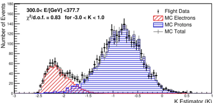
where the sum runs over the logs of the layer and xcis the coordinate of the reconstructed particle track in the first TASC layer, xjand ∆Ej are the coordinate of the center and the energy deposit in the j-th PWO log, respectively. In order to minimize the impact of noise in each chan-nel, a 3 MIP threshold is applied to all channels for FE and RE. While these prescriptions significantly reduce the proton rejection power in the low energy region, they are adopted to make our analysis much less sensitive to possible fluctuation in detector noise. Based on the val-ues defined here, a K-estimator is defined as follows:
K = log10(FE) +1 2RE.
An example of K-estimator distributions is shown in Fig 2, where clear separation of the electron peak from the proton peak is achieved.
K Estimator (K) -3 -2.5 -2 -1.5 -1 -0.5 0 0.5 1 Number of Events 0 20 40 60 80 100 120 140 160 180 Flight Data MC Electrons MC Protons MC Total 300.0< E/[GeV] <377.7 /d.o.f. = 0.83 for -3.0 < K < 1.0 2 χ
FIG. 2. An example of K-estimator distribution in the 300 <
E < 378 GeV bin. The reduced chi-square of the fit in the
K-estimator range from -3 to 1 is 0.83.
Because RE is a second moment parameter, it is sensi-tive to the tail of lateral distribution affected by multiple Coulomb scattering. In order to reproduce FD distri-butions with EPICS, the MC program was intensively
checked and tuned. Most importantly, we have adopted the “El hin” model[13], implemented in EPICS, which provides an improved treatment of multiple Coulomb scattering with respect to the default Moliere model in EPICS.
Multivariate Analysis using Boosted Decision Trees
Definition of discriminating variables - We use
the multivariate analysis toolkit TMVA [14] available in the Root analysis framework to train boosted decision trees (BDT) and to calculate BDT response. The dis-criminating variables for BDT are selected from the fol-lowing list in an energy dependent way where the vari-ables with very good agreement between MC and FD have been chosen:
(1) A parameter characterizing lateral shower develop-ment in TASC (RE);
(2) A parameter characterizing longitudinal shower de-velopment in TASC (FE);
(3) IMC Shower concentration (CIMC−Y8);
(4) Parameters to fit longitudinal shower development in TASC:
a. shower maximum (α/b);
b. shower attenuation constant (b); c. 5% shower depth (t5%);
d. goodness of fit (χ2 TASC);
(5) Parameters to fit the pre-shower development in IMC:
a. constant in exponential fit (p0);
b. slope in exponential fit (p1);
c. goodness of fit (χ2 IMC);
where CIMC−Y8 is defined as the sums of the energy
de-posits of±9 fibers (1 Moliere radius for tungsten) along the reconstructed shower axis divided by the sum of all 448 fibers in the bottom IMC layer (Y8). TASC shower profile fit and IMC shower profile fit are performed ac-cording to the following parameterizations [15]:
dE dt = E0 b(α+1) Γ(α + 1)t αe−bt, dE dt = e p0+p1t,
where t is the depth in radiation length along the re-constructed shower axis measured from the position of first impact. The fitting parameters are used as discrimi-nating variables for BDT. The discrimidiscrimi-nating variables actually used are: (1)–(3) below 100 GeV, all except for (3),(4)-b in 100–500 GeV, all except for (3) above 500 GeV. In the low energy region below 100GeV, it
is sufficient to use only the first 3 discriminating vari-ables. However, at present, simulation of backscattering by EPICS above 100 GeV needs a deeper study as the tribution of shower concentration in IMC shows some dis-crepancy with respect to the flight data. Therefore, (3) is not used as discriminating variable above 100 GeV. In addition, (5) is not used in the lower energy region where it shows some inconsistencies. Possible secondary effects that may arise even when removing the above variables from the set of discriminating variables have been stud-ied. We have carried out a comparison with results based on Geant4 [16] and have estimated the related systematic uncertainties in the following section.
Training and application of BDT - In the BDT
analysis the whole set of MC data (electrons and pro-tons) is equally subdivided into training and test samples. During the training, supervised learning is performed us-ing particle identification as supervisory signal. While training is carried out only using the former dataset, test samples are actually used to estimate the efficiency for electrons and contamination of protons. In order to take advantage of exact shower development for electrons as a function of energy and event geometry, each training was carried out separately with a specific geometry condition and fine energy binning with a bin-width factor of 101/25. The decision trees with a depth of 20 are generated 100 times with updated weights for mis-identified events, and are used to calculate BDT response using the weighted average of all the trees.
Background Contamination
Besides K-estimator and BDT response specifically se-lected for proton rejection, most of the pre-selection cuts have also some capability in proton rejection. To illus-trate this, (a) electron and (b) proton efficiencies as a function of energy are shown in Fig. 3 for each important selection step. By combining trigger, track reconstruc-tion and all the pre-selecreconstruc-tion cuts, efficiency for protons is already less than 1% level, and electron identification adds another factor of 10 to 100 while preserving most of electrons. It should be noted that the proton effi-ciency shown in Fig. 3 is the effieffi-ciency with respect to the primary proton energy, while the rejection power of 105 mentioned earlier is the rejection power with respect
to potential background for the electron measurement, i.e. the integral of the assumed proton flux above the electron energy.
To extract the proton contamination in the final sam-ple of electron candidates, template fitting of the crit-ical distribution for electron/proton identification (K-estimator defined in the previous section for simple cut analysis and BDT response for MVA) was used where normalization factors for MC electrons and MC protons are included as fitting parameters. The cut position
cor-responding to 80% efficiency is determined by using the MC electron distributions, and the contaminating pro-tons are derived as the expected absolute number of MC proton events passing the electron selection with relative normalization factor. In this way, it is possible to sub-tract the background protons regardless of the spectral shape of electrons.
The proton spectrum adopted to calculate contamina-tion into each energy bin is derived from the published measurements and flux parameterization of AMS-02 [17]
Energy [GeV] 20 30 40 102 2×10² 103 2×10³ Electron Efficiency 0.1 0.2 0.3 0.4 0.5 0.6 0.7 0.8 0.9 1 (1) Offline Trigger
(2) Geometrical Condition & (3) Track Quality Cuts (4) Charge Selection
(5)&(6) Shower Development Consistency Cuts K-estimator Cut 80% BDT Cut 80% (a) Energy [GeV] 20 30 40 102 2×10² 103 2×10³ Proton Efficiency -5 10 -4 10 -3 10 -2 10 -1 10 1 (b)
FIG. 3. (a) Electron efficiency as a function of energy for each important selection step. (b) Same for protons. Black, green, yellow, blue and red histograms show the efficiency after (1) offline trigger, (2) geometrical condition with (3) track quality cuts, (4) charge selection, and (5)&(6) shower development consistency cuts, K-estimator cut with 80% efficiency, BDT cut with 80% efficiency, respectively.
and CREAM-III [18]. Each event in MC is weighted con-sidering the difference between the parameterized and generated (E−1) spectrum as a function of primary en-ergy, which is also taken into account in the statistical error calculation for the MC sample by summation of the squared weights. As expected, BDT showed better per-formance especially above TeV range where background contamination is a factor of 2–3 less than a cut driven analysis. Note that the statistics available for the former method is almost one half of the latter due to the needs of training.
SYSTEMATIC UNCERTAINTY
Contributing factors to systematic uncertainties in-clude:
1. energy scale;
2. geometrical acceptance; 3. observational live time; 4. radiation environment at ISS; 5. long-term stability;
6. pre-selection;
(a) track reconstruction; (b) pre-selection efficiency; 7. electron identification;
(a) electron identification efficiency; (b) background contamination; 8. MC model dependence.
Each item except for energy scale uncertainty has been included in the total systematic uncertainty band. In the following a summary of the main topics is provided while discussions about energy scale uncertainty and BDT analysis stability are provided in the main text.
Observational Live Time
Measurements of dead time is the key to retrieve ob-servational live time. In CALET observations, there is around 5–6 ms of dead time occurring for data acquisi-tion of each event. Although the dead time could vary due to periodic tasks and load of data acquisition, it is accurately counted event by event with a scaler based on 15.625 µs clock while readout of the scaler is carried out periodically every 1 sec. On the other hand, possible error in dead time measurements would be seen as a de-pendence on the data acquisition rate because the errors would cumulate.
To estimate such effects, the whole observation period is divided into 4 sub-periods as (i) live time fraction larger than 0.88, (ii) 0.72–0.88, (iii) 0.60–0.72 and (iv) less than 0.60. Then, the spectrum for each period is calculated
and compared with the one from the whole period by tak-ing the relative difference. While small, some dependence on the live time fraction was observed. To estimate sys-tematic errors due to live time measurements, a limited energy range can be used because the live time accumu-lation for the flux calcuaccumu-lation is practically energy inde-pendent. From the distribution of the relative difference in all the cases and all bins between 20 GeV to 100 GeV, the standard deviation of 3.4% is obtained. While the result includes statistical fluctuations, the uncorrected standard deviation of 3.4% is considered as systematic error due to live time measurements. Note however that the dependence might be due to some hidden parameters since there is no simple correlation (monotonical increase or decrease) between live time fraction and relative differ-ence of spectrum. It could be due to the fact that in the 4 periods the contiguous time intervals selected are not much larger than dead time sampling interval of 1 sec. In such case, the first and last events in the time interval introduce an approximation error which is not present in the regular flux. While this possibility should be further investigated in the future, the current estimate of sys-tematic uncertainty due to the observed discrepancy is on the conservative side.
During ground test, accuracy of live time measure-ments were measured and validated with 0.2% precision by using random trigger system and equivalent model of Mission Data Controller (MDC) in various trigger con-ditions and characteristic buffer usage status. The de-pendence on live time fraction in FD is larger than the results of ground test. However, the largest discrepancy, i.e. sub-period (iii), corresponds to only 3.5% of the total live time, therefore a systematic uncertainty of 3.4% is comfortably conservative.
Long-term Stability
To confirm the long-term stability of detector sensi-tivity, spectrum stability was investigated by dividing the whole observation period into 4 sub-periods for every 157 days (in total 627 days and thus the last period covers 156 days). There are some variations at the level of 1–2% in the first observation period. The long-term variation of detector gain is monitored and corrected by MIP cali-bration carried out on orbit at regular intervals and there is no systematic deviation in the calibration results. Even though very small, the reason for the long-term variation in the spectrum is not well understood. The systematic error related to long-term stability is evaluated in the 20–100 GeV energy range in the same way as live time, resulting in a systematic uncertainty of 1.4%. While it is mostly consistent with pure statistical fluctuation which is evaluated as 1.4%, a systematic uncertainty of 1.4% is conservatively associated with long-term stability.
Electron Identification
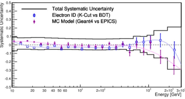
The procedure to identify electrons from the over-whelming proton flux (a factor of the order of 1000 larger than the electron flux in the TeV region) and to subtract the remaining proton background from the final electron candidates are the most important source of systematic uncertainty. One of the main difficulties in the evalu-ation of such systematic effect is the strong correlevalu-ation between electron efficiency and proton rejection power. In the present analysis, the final result above 500 GeV is obtained using BDT which has superior proton rejection capability in the higher energy region. However, care needs to be taken since the selection criteria of BDT are formed by complex multi-parameter cuts making it dif-ficult to disentangle the possible issues. On the other hand, a simple two parameter cut is used to derive the final spectrum below 500 GeV to maximize statistics of MC protons and to allow fitting of the background con-tamination. Note that smooth variation of background contamination is not guaranteed in BDT because inde-pendent training of trees in each energy bin. Due to the very high statistics of electron candidates in the low-energy region, MC statistics is the largest source of sta-tistical fluctuation. As both methods should be valid as long as our MC description is correct, the simple cut analysis and BDT results are compared to verify their consistency. The relative difference between K-estimator cut and BDT analyses is shown as blue points in Fig. 4 as a function of energy, together with the log-polynomial fit (light blue line) that has been used to estimate the bin-by-bin systematic uncertainty. Overall, they are con-sistent with each other. While BDT has better rejection power and thus is affected by smaller contamination in the TeV region, BDT uses a complicated multi-parameter selection optimization in each energy bin as mentioned, and it is difficult to understand its systematics in simple terms. On the other hand, the simple cut analysis relies totally on one parameter for electron identification but suffers from larger BG contamination. Therefore, the fact that there is a relatively small discrepancy of the order of the 3% (5%) below (above) 500 GeV, between these two analyses provides an important consistency check. The relative difference fitted with log-polynomial func-tion is included in the systematic uncertainty taking into account the sign of the difference for each energy bin.
MC Model Dependence
By simulating important detector response such as pedestal noise and photoelectron statistics, important distributions like energy deposit of minimum ionizing particles are well reproduced by MC. In addition, de-tector geometry is reproduced in detail using CALET CAD model. Overall, an agreement between FD and
Energy [GeV] 10 20 30 40 50 60 2 10 2 10 × 2 3 10 3 10 × 2 3 10 × 3 Systematic Uncertainty -0.5 -0.4 -0.3 -0.2 -0.1 0 0.1 0.2 0.3 0.4 0.5
Total Systematic Uncertainty Electron ID (K-Cut vs BDT) MC Model (Geant4 vs EPICS) Total Systematic Uncertainty Electron ID (K-Cut vs BDT) MC Model (Geant4 vs EPICS)
FIG. 4. Energy dependence of systematic uncertainties in electron identification methods (K-estimator vs BDT) and MC models (Geant4 vs EPICS), which are fitted with 7th-order log-polynomial to avoid too much statistical fluctua-tions while preserving possible energy dependent structures. Fit functions are shown as curves and are used to estimate energy dependent systematic uncertainties. Note that uncer-tainties in electron identification are estimated by (BDT − K-estimator) below 500GeV and (K-estimator− BDT) above 500GeV.
MC is achieved at fairly high level, though not perfect. Specifically, backscattering of high energy protons and electromagnetic shower attenuation below a few hundred GeV are examples of such small discrepancies. To eval-uate the uncertainty coming from the incompleteness of our MC model based on EPICS, comparison with a dif-ferent MC model based on Geant4 was carried out. The detector model used in Geant4 version is mostly iden-tical to CALET CAD model. Geant4 version employs FTFP BERT as physics list which is recommended for the simulation of high energy showers. The important points in comparison between Geant4 and EPICS are:
- Backscattering: EPICS produces less backscatter-ing with respect to FD while Geant4 generates too much backscattering. Both are not in very good agreement with FD, but their discrepancies are on opposite sides with respect to FD.
- Shower attenuation constant: it is in good agree-ment with FD in Geant4, while showing discrep-ancy in EPICS below a few hundred GeV.
Therefore, the difference between Geant4 and EPICS can be considered as upper limit on possible effects of physics processes which are not perfectly simulated, making it possible to quote it as systematic uncertainty related to physics process simulation. The relative difference be-tween the spectrum derived with Geant4 and that de-rived with EPICS is shown as purple points in Fig 4, and fitted with log-polynomial. The resultant function is used to quote the systematic uncertainty considering the sign of difference in each energy bin. The estimated systematic error due to MC model which is within a few percent below 1 TeV and below 25% in the TeV region where statistical accuracy dominates the estimation.
TABULATED FLUX
The measured all-electron flux including statistical and systematic errors is tabulated in Table I.
TABLE I. Summary of CALET electron plus positron spec-trum. For the flux, the first and second errors represent the statistical uncertainties (68% confidence level) and systematic uncertainties, respectively, while the systematic uncertainty on the energy scale is not included.
Energy Bin Mean Energy Flux
(GeV) (GeV) (m−2sr−1s−1GeV−1) 10.6–11.9 11.3 (1.546± 0.005+0.117−0.108)× 10−1 11.9–13.4 12.6 (1.065± 0.004+0.072−0.055)× 10−1 13.4–15.0 14.2 (7.404± 0.026+0.500−0.383)× 10−2 15.0–16.9 15.9 (5.073± 0.020+0.344−0.261)× 10−2 16.9–18.9 17.8 (3.504± 0.015+0.238−0.180)× 10−2 18.9–21.2 20.0 (2.457± 0.012+0.174 −0.136)× 10−2 21.2–23.8 22.5 (1.679± 0.009+0.119−0.093)× 10−2 23.8–26.7 25.2 (1.159± 0.007+0.082−0.066)× 10−2 26.7–30.0 28.3 (7.988± 0.037+0.568−0.457)× 10−3 30.0–33.7 31.7 (5.411± 0.029+0.354−0.287)× 10−3 33.7–37.8 35.6 (3.715± 0.023+0.243 −0.197)× 10−3 37.8–42.4 39.9 (2.620± 0.018+0.163 −0.139)× 10−3 42.4–47.5 44.8 (1.794± 0.014+0.111−0.095)× 10−3 47.5–53.3 50.3 (1.261± 0.011+0.075−0.067)× 10−3 53.3–59.9 56.4 (8.883± 0.087+0.525−0.475)× 10−4 59.9–67.2 63.3 (6.129± 0.068+0.338−0.328)× 10−4 67.2–75.4 71.0 (4.162± 0.053+0.230 −0.223)× 10−4 75.4–84.6 79.7 (3.009± 0.043+0.158 −0.166)× 10−4 84.6–94.9 89.4 (2.023± 0.033+0.106−0.111)× 10−4 94.9–106.4 100.4 (1.45 ± 0.03+0.07−0.08)× 10−4 106.4–119.4 112.6 (9.94 ± 0.21+0.51−0.57)× 10−5 119.4–134.0 126.3 (7.00 ± 0.16+0.34−0.41)× 10−5 134.0–150.4 141.8 (4.99 ± 0.13+0.25 −0.29)× 10−5 150.4–168.7 159.1 (3.57 ± 0.10+0.17−0.21)× 10−5 168.7–189.3 178.8 (2.53 ± 0.08+0.12−0.15)× 10−5 189.3–212.4 200.1 (1.72 ± 0.06+0.08−0.10)× 10−5 212.4–238.3 224.5 (1.14 ± 0.05+0.05−0.07)× 10−5 238.3–267.4 252.4 (8.01 ± 0.39+0.39−0.46)× 10−6 267.4–300.0 282.9 (5.72 ± 0.31+0.28 −0.33)× 10−6 300.0–336.6 317.6 (3.93 ± 0.24+0.20−0.22)× 10−6 336.6–377.7 355.9 (2.80 ± 0.19+0.15−0.15)× 10−6 377.7–423.8 400.3 (1.90 ± 0.15+0.11−0.10)× 10−6 423.8–475.5 446.7 (1.14 ± 0.11+0.06−0.06)× 10−6 475.5–598.6 530.3 (7.18 ± 0.56+0.40−0.48)× 10−7 598.6–753.6 665.1 (3.13 ± 0.33+0.28 −0.18)× 10−7 753.6–948.7 848.8 (1.84 ± 0.23+0.16−0.16)× 10−7 948.7–1194.3 1065.4 (9.39 ± 1.46+0.92−1.04)× 10−8 1194.3–1892.9 1489.2 (2.33 ± 0.44+0.36−0.34)× 10−8 1892.9–3000.0 2432.8 (4.51 ± 1.60+0.89−1.28)× 10−9
[1] K. Yamaoka et al., in Proc. 7th Huntsville Gamma-Ray
Burst Symposium, GRB 2013 (2013) p. 41.
[2] P. S. Marrocchesi et al., Nucl. Instrum. Methods Phys Res., Sect. A 659, 477 (2011).
[3] P. S. Marrocchesi et al., in Proc. of 33rd international
cosmic ray conference (ICRC2013) 362 (2013).
[4] P. S. Marrocchesi et al., in Proceeding of Science
(ICRC2017) 156 (2017).
[5] Y. Akaike et al., in Proceedings of Science (ICRC2017)
181 (2017).
[6] M. Mori et al., in Proc. of 33rd international cosmic ray
conference (ICRC2013) 248 (2013).
[7] Y. Akaike et al., in Proceedings of the 32nd ICRC, Vol. 6 (2011) p. 371.
[8] Y. Akaike et al., in Proc. of 33rd international cosmic ray
conference (ICRC2013) 726 (2013).
[9] Y. Akaike et al., in Proceeding of Sciences (ICRC2015)
613 (2015).
[10] T. Niita, S. Torii, Y. Akaike, Y. Asaoka, K. Kasahara,
et al., Adv. Space Res. 55, 2500 (2015).
[11] F. Palma et al., in Proceedings of Science (ICRC2015)
1196 (2015).
[12] L. Pacini, Y. Akaike, et al., in Procceeding of Science
(ICRC2017) 163 (2017).
[13] J. Femindez-Varea, R. Mayo, J. Bar, and F. Salvat, Nucl. Instrum. Methods B73, 447:473 (1993).
[14] A. Hocker et al., in Proc. Sci., ACAT2007 (2007) p. 040. [15] E. Longo and I. Sestili, Nucl. Instrum. Methods 128, 283
(1975).
[16] S. Agostinelli et al., Nucl. Instrum. Methods Phys. Res.
A506, 250 (2003).
[17] M. Aguilaret al., Phys. Rev. Lett. 114, 171103 (2015).
![FIG. 1. CALET instrument assembly showing the main calorimeter, and the Gamma-ray Burst Monitor (CGBM), composed of a hard X-ray monitor and a soft gamma-ray mon-itor [1], installed in a JEM standard payload with a size of 1850mm(L) × 800mm(W) × 1000mm(H)](https://thumb-eu.123doks.com/thumbv2/123dokorg/4647973.41962/1.918.142.389.569.804/instrument-assembly-showing-calorimeter-monitor-composed-installed-standard.webp)