Research Article
Minimal Diagnosis and Diagnosability of Discrete-Event
Systems Modeled by Automata
Xiangfu Zhao ,
1Gianfranco Lamperti ,
2Dantong Ouyang ,
3and Xiangrong Tong
11School of Computer and Control Engineering, Yantai University, Yantai 264005, China 2Department of Information Engineering, University of Brescia, Brescia 25123, Italy 3College of Computer Science and Technology, Jilin University, Changchun 130012, China
Correspondence should be addressed to Xiangfu Zhao; [email protected] and Xiangrong Tong; [email protected] Received 13 September 2019; Revised 13 December 2019; Accepted 7 January 2020; Published 18 February 2020 Guest Editor: Viet-Thanh Pham
Copyright © 2020 Xiangfu Zhao et al. This is an open access article distributed under the Creative Commons Attribution License, which permits unrestricted use, distribution, and reproduction in any medium, provided the original work is properly cited. In the last several decades, the model-based diagnosis of discrete-event systems (DESs) has increasingly become an active research topic in both control engineering and artificial intelligence. However, in contrast with the widely applied minimal diagnosis of static systems, in most approaches to the diagnosis of DESs, all possible candidate diagnoses are computed, including nonminimal candidates, which may cause intractable complexity when the number of nonminimal diagnoses is very large. According to the principle of parsimony and the principle of joint-probability distribution, generally, the minimal diagnosis of DESs is preferable to a nonminimal diagnosis. To generate more likely diagnoses, the notion of the minimal diagnosis of DESs is presented, which is supported by a minimal diagnoser for the generation of minimal diagnoses. Moreover, to either strongly or weakly decide whether a minimal set of faulty events has definitely occurred or not, two notions of minimal diagnosability are proposed. Necessary and sufficient conditions for determining the minimal diagnosability of DESs are proven. The relationships between the two types of minimal diagnosability and the classical diagnosability are analysed in depth.
1. Introduction
In recent years, several disasters, including the nuclear leakage that occurred in Fukushima (Japan) in 2011 and the blackout that occurred in nearly the entire country of India in 2012, have greatly threatened the safety of society and even the lives of many people. To prevent such disasters, determining faulty events/components is a very important topic. To this end, model-based fault diagnosis techniques may be very effective. Nonlinear science is a new interdisciplinary subject which studies the common problems proposed by nonlinear interaction widely existing in various disciplines, especially in complex networks [1–4], system control [5–7], secure communication [8–10], chaotic systems [11], random number generators [12, 13], discrete-event systems (DESs) [14], and other fields. The creative work on the diagnosis/ diagnosability of DESs, presented in [15, 16], with the originally proposed concept of a diagnoser, model-based diagnosis, and diagnosability have attracted more and more
attention, as indicated by the large number of methods and techniques proposed in the literature, including [17–26]. Because of the intractable complexity of reasoning of the global DES model and the corresponding centralized diagnoser, decentralized approaches were proposed in [27–29]. More recently, fuzzy diagnoser/diagnosability [30, 31] or the stochastic diagnoser/diagnosability/prog-nosability [32–35] has been studied, with fuzzy or stochastic information being injected into an automaton that models a DES. In addition to diagnoser-based approaches for the diagnosis of DESs, a history-based approach [36, 37] and a consistency-based approach [38] to the diagnosis of DESs have also been presented.
However, as far as we know, one of the current main problems is that, in most approaches to diagnosing DESs, all possible candidate diagnoses are derived, even if many candidates are proper supersets of some other candidates. In other words, nonminimal (redundant) diagnoses are generated.
Volume 2020, Article ID 4306261, 17 pages https://doi.org/10.1155/2020/4306261
In this paper, we extend the idea of a minimal diagnosis, first presented in [39], via additional theoretical analyses, formal proofs, examples, and comparisons with related work.
Example 1. Among candidate diagnoses (sets of possible
faulty events) f 1, f 2, f3, f 1, f2, f3, f 1, f3, f4, and
f2, f3, f4
, only {f1} and f 2, f3are minimal according to
the set-inclusion relationship, as all other candidates contain
f1
or f 2, f3and include additional faults (f2and/or f3
and/or f4). Minimal diagnosis differs from
dinality diagnosis. In our example, the only minimal-car-dinality diagnosis is f 1. In this paper, we focus on minimal diagnosis rather than minimal-cardinality diagnosis. In addition, in our example, even if we cannot definitely know
whether f4 has occurred or not, we know that minimal
diagnoses {f1} and {f2, f3} are generally more probable
than others.
In theory, all possible fault sets need to be diagnosed. However, considering a scenario like Example 1, although there are a large number of possible candidate diagnoses that can explain the current observation sequence, there may exist set-inclusion relationships among some of them.
The two principles of parsimony and joint-probability distribution, which are briefly described as follows:
(i) The principle of parsimony: also called “Occam’s razor” [40], parsimony is a principle of succinctness often adopted in logic and problem solving which states that, among competing hypotheses, the hy-pothesis with the fewest assumptions should be selected. The principle of parsimony has also been introduced for the minimal diagnosis of static sys-tems [41].
(ii) The principle of joint-probability distribution: a widely used assumption in the literature, in this paper, a joint-probability distribution means that each fault is independent of one another and that the prior probability of each fault is equal.
Minimal diagnoses (based on the set-inclusion rela-tionship (for instance, we assume that there are three candidate diagnoses f 1, f 1, f2, and f 2, f3, f4, f5. Then, f 1and f 2, f3, f4, f5are minimal diagnoses, even if f 2, f3, f4, f5has a bigger cardinality than f 1, f2but without a set-inclusion relationship between them.)) are more likely than the corresponding nonminimal ones. As a result, just like the minimal diagnosis of static systems [41, 42], determining only the minimal diagnoses of DESs is bound to reduce the complexity, as additional nonminimal diagnoses are not considered.
The benefit of a minimal diagnosis is related to both cognition and computation. Cognition is relevant to the human who is responsible for the monitoring of the DES. Consider, for instance, the operator in the control room of a power network, who is responsible for the correct behaviour of the network. When a misbehaviour occurs, such as a short circuit on a transmission line, several actions can be trig-gered by the protection system to isolate the shorted line,
e.g., opening breakers and reconfiguring the power load to avoid a blackout. If the reaction of the protection system is abnormal, a possibly large number of alarms and messages will be generated. Since the operator is expected to activate specific recovery actions, it is essential that the (possibly overwhelming) stream of information generated by the system, namely, the observation, be interpreted correctly under stringent time constraints. This is why automated diagnosis becomes a key factor in supporting the operator in performing his/her critical job. To this end, the diagnosis engine may generate diagnosis information in a relatively short amount of time. Specifically, a set of candidate diag-noses are presented to the operator, who is expected to make critical decisions regarding the safety of the involved pop-ulation. However, if the number of candidates is large, the operator may be confused about which diagnoses should deserve more attention. Choosing minimal diagnoses is a good heuristic, as they are more probable and, as such, more worthy of attention.
Computation involves the efficient generation of can-didate diagnoses. Since a key factor in real applications of automated diagnosis is the time response, that is, the delay between the occurrence of a faulty event and the generation of candidate diagnoses, it is of paramount importance that the diagnosis engine is not only effective but also efficient. Being free of the burden of nonminimal candidates, minimal diagnosis allows the diagnosis engine to be more efficient compared with nonminimal diagnosis with respect to both processing speed and memory space.
In summary, the main contribution of the paper is that the theoretical concepts of minimal diagnosis and minimal diagnosability of DESs are proposed, and meanwhile, the minimal diagnosis of DESs is not a purely academic exercise; it may drive attention to the actual cause of a misbehaviour effectively (cognition) and efficiently (computation).
The rest of the paper is organized as follows. The ter-minology and preliminary concepts related to the model-based diagnosis of DESs are given in Section 2. Several novel concepts, including minimal diagnosis, minimal diagnoser, and minimal diagnosability of DESs, are presented in Sec-tion 3. Related work is discussed in SecSec-tion 4. Conclusions and future work are presented in Section 5.
2. Background
In this section, the classical notions of the diagnosis, diagnoser, and diagnosability of DESs [16] are recalled.
2.1. Classical Diagnosis of DESs. A DES is a deterministic
finite state machine (FSM), namely, G � (Q, Σ, T, q0), where
Q is the set of states.
Σ is the set of events, including two disjoint sets of observable events (Σo) and unobservable events (Σuo); f� f 1, f2, . . . , fm(for the sake of simplicity, the classification (types) of faults in [16] is disregarded in this paper), with f⊆ uo, is the set of faulty events to be inferred, while (Σuo− Σf)is the set of events that are both unobservable and nonfaulty.
T⊆ Q × Σ × Q is the set of transitions, where a tran-sition from state q to state q′, when event e is activated
on state q, is equivalently denoted by (q, e, q′)∈ T,
q⟶e q′, or T(q, e) � q′.
q0∈ Q denotes the initial state of the system.
The behaviour of G consists of all possible traces
gen-erated from q0to some state in G, which form a prefix-closed
language L(G), abbreviated as L, with L ⊆ Σ∗(Σ∗is the set of all possible strings composed of events in Σ, including the empty string ε). For simplicity, we assume that language L is live, that is,
For each state q ∈ Q, there exists at least one event
σ ∈ Σ such that q ⟶σ q′ holds, where q′∈ Q (with q′
being nonnecessarily different from q).
In addition, similar to [16], we assume that there does not exist any cycle of unobservable events, that is,
For any cycle q1⟶
σ1
q2⟶σ2 · · · qk−1⟶σk−1 qk ⟶σk q1
(k ≥ 1), qi∈ Q, and σi∈ Σ (i ∈ [1 · · · k]), there exists at least one event σj (j ∈ [1 · · · k]) such that σj ∈ Σo.
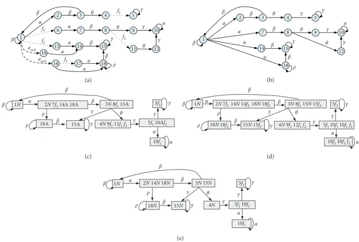
Example 2. Outlined in Figure 1(a) is the diagrammatic
representation of a DES model G, where Σo�{α, β, c, θ, ρ},
Σf� f 1, f2, and Σuo�σuo1,σuo2∪ Σf.
We denote the empty trace as ε and extend one transition event to a string of transition events as follows:
q⟶ε qalways holds
For s ∈ Σ∗ and σ ∈ Σ, q ⟶s σ q′ holds whenever
q⟶s q″ and q″⟶σ q′hold for q″∈ Q
Denoting a transition in which the entered state is missing, q ⟶s indicates that, for s ∈ Σ∗, there exists at
least one state q′∈ Q such that q ⟶s q′ holds.
The notation L/s represents the postlanguage of L after string s ∈ L, that is, L/s � t | t ∈ Σ{ ∗, st∈ L}.
Two types of projection are given: PrjΣo(on observation)
and PΣf (on faults). Assuming that σ ∈ Σ and s ∈ Σ
∗, PrjΣo:Σ
∗⟶ Σ∗
o represents how a trace is projected onto a
sequence of observable events:
PrjΣo(sσ) � PrjΣo(s)PrjΣo(σ). (1)
Conversely, Prj−Σ1o(so) � s | s ∈ L, PrjΣo(s) � sodenotes
the set of traces whose projection equals so(note here that
Prj−1
Σo(PrjΣo(so))may not equal so).
PΣ
f: Σ
∗⟶ 2Σf denotes how a (possibly empty) trace
s∈ Σ∗ is mapped onto a set of faults:
PΣ
f(s) � fi fi
∈ Σf, fi∈ s
. (2)
Example 3. Let s � af1bcf2, f 1, f2⊆ Σf, and a, b, c{ }⊆ Σo. We have PrjΣo(s) � abcand PΣf(s) �{f1, f2}.
Let se denote the last event of a nonempty trace s ∈ Σ+,
where Σ+�Σ∗− { }, and F ⊆ Σf. Then, SFε � s | s{ ∈ L,
PΣ
f(s) � F, se ∈ F} denotes the set of all traces ending with
one fault of F and containing all the faulty events of F.
We use L(G, q) to denote all traces in G starting from state q. Let Lo(G, q) � s | s ∈ L(G, q), s � uσ, u ∈ Σ∗uo,
σ ∈ Σo}denote all traces starting from state q up to the first
observable event and Lσ(G, q) �{s | s ∈ Lo(G, q), se �σ}
denote all traces starting from q up to the first observable event σ.
Based on G � (Q, Σ, T, q0), an FSM Go�(Qo, Σo, To, q0) (in general, nondeterministic (a nondeterministic FSM is a state in G which may reach more than one state via the same transition event. Accordingly, in Figure 1(b), state 1 can reach four different states (2, 7, 14, and 18) via the same observation α)) is defined as follows:
Qo� q 0
∪ q ′| q⟶σ q′∈ T, σ ∈ Σo} denotes both q0 and all observable states.
To⊆ Qo×Σo× Qodenotes the set of transitions, defined as follows: qo,σ, qo′ ∈ To, iff T qo, s � qo′, s∈ Lσ G, q o . (3) As such, L(Go) � t | t �Prj Σo(s), s∈ L .
Example 4. With reference to Example 2, Figure 1(b)
presents a diagrammatic representation of Go, with G
be-ing displayed in Figure 1(a).
Based on the abovementioned notions, the notion of the diagnosis of a DES is given in Definition 1.
Definition 1. Let G � (Q, Σ, T, q0) be a DES, L be the
corresponding language of G, and obs ∈ Σ∗o be the current
observation sequence for G. A subset F ⊆ Σf is called a
candidate diagnosis (or just a diagnosis) of a DES for ob-servation sequence obs (written as F ⇝ obs) iff there is a
string of events s ∈ L with se∈ Σo such that PΣf(s) �
F∧ PrjΣo(s) �obs.
In other words, a diagnosis of a DES is a set of faulty events (unlike the diagnosis of static systems (e.g., [41, 42]), where a diagnosis is defined as a set of faulty components.) in a trace whose mapping onto observable events equals only the current observation sequence obs. Note that the
con-dition se∈ Σo must be satisfied in the definition, as we
generally use the currently received observation sequences immediately after the DES fails to work properly to infer a set of faults to explain observation obs (this is also a funda-mental principle of finding the diagnosis of DESs).
Example 5. With reference to Example 2, for the DES G
displayed in Figure 1(a), if we get the current observation sequence obs � αβθ, then all candidate diagnoses are ∅,
f1
, and f 1, f2, with αβθ, f1αβθ, and f1αβf2θ being the corresponding traces of events, respectively.
2.2. Classical Diagnoser for DESs. To generate candidate
diagnoses, the diagnoser-based approach introduced in [16] is used.
Let Δ � 2Σf∪ A{ }be all possible fault labels, with each label
being a set of faulty events. N is used as an alias for the empty fault set (to indicate a normal state). A is interpreted as
“ambiguous” (that is, we cannot be sure that some faults have definitely occurred).
Starting from Go� (Qo,Σo, To, q
0), the classical
diag-noser Gdfor G is a deterministic FSM:
Gd� q d,Σo, Td, q0d, (4) where
qd⊆ 2(Qo×Δ)
is the set of states.
q0
d� (q 0, N)(since the fault label associated with q0is
N, G is assumed to be normal at the initial state.) Any
state qd∈ qdis reachable from q0
dvia transitions in Td, written as qd�{(qo 1, l1), . . ., (qon, ln)}, where q o i ∈ Q oand
li∈ Δ (that is, liis in the form of either N or a nonempty
subset of Σf∪ A{ }). In subsequent set-theoretic
oper-ations in the minimal diagnoser, we replace N with the empty set ∅.
The range function R: qd×Σo⟶ qd is defined as
follows: R qd,σ � ∪ qo,l ( )∈qd ∪ s∈Lσ(G,qo) T qo, s,LP qo, l, s ⎛ ⎝ ⎞⎠, (5)
where LP: Qo×Δ × Σ∗⟶ Δ denotes the fault label
propagation function. Given qo∈ Qo, l∈ Δ, and s ∈ Lo(G,
qo), fault label l is propagated by LP over string s from qoin the following way:
LP qo, l, s � f ifi∈ l ∨ fi∈ s. (6)
Then, the label correction function LC: qd⟶ qd is
defined as follows: LC qd �qo, l qo, l∈ qd, and ∄ qo, l′∈ qdwith l′≠ l∪ q o, A{ }∪ li 1∩ · · · ∩ lik| qo, li 1 , . . . , qo, li k ∈ qd, lv≠ lw, v, w∈ i1, . . . , ik, v≠ w, k ≥ 2. (7)
The label correction function LC and the label A can be explained as follows. When the system moves along trace s
and transitions from some state into a state qowith at least
two different fault labels, we cannot be sure that some faults
9 10 7 8 6 5 3 4 2 β β f1 f2 f2 f1 f2 β β γ γ γ γ ρ α α α β β α α α α θ θ θ 1 11 12 14 15 13 17 18 16 19 σuo1 σuo2 (a) β β β β β β γ γ γ γ γ ρ α α α α α θ θ 9 10 7 8 5 3 4 2 1 12 14 15 18 θ (b) γ γ γ γ γ ρ ρ β β β β α α α θ 2N 7f1 18A 15A 1N 14A 18A 3N 8f1 4N 9f1 5f1 5f1 10f1 10Af1 12f1 f2 15A (c) γ γ γ γ γ ρ ρ β β β β α α α θ 2N 7f1 1N 14N 14f218N 18f2 18N 18f2 3N 8f115N 15f2 15N 15f2 5f1 4N 9f112f1 f2 5f110f110f1 f2 10f110f1 f2 (d) γ γ γ γ γ ρ ρ β β β β α α α θ 1N 2N 14N 18N 3N 15N 4N 15N 18N 5f1 5f110f1 10f1 (e)
Figure 1: A DES and its related variant diagnosers: (a) DES model G. (b) Nondeterministic FSM Gofor G. (c) Classical diagnoser Gdfor G.
have definitely occurred; therefore, we use label A to refer to this scenario.
The transition function Td: qd×Σo⟶ qdis defined as
follows: qd2 � Tdq1d,σ⟺ q2d�LC R q 1 d,σ . (8)
In other words, assuming that the current state in diagnoser Gdis q1
d, while the next observable event is σ, we
generate the new state q2
dof Gdin the following way:
(1) For each (qo, l)∈ q1
d, compute the set S(q
o,σ) of
reachable states of G from qo using observation σ:
S(qo,σ) � T(qo, uσ) | u ∈ Σ∗
uo, and σ ∈ Σo
(note
here that S(qo,σ) is a finite set of observable
states, as we have made an assumption (in Section 2.1) that there does not exist any cycle of unobservable events [16]).
(2) Given qo′∈ S(qo,σ) with T(qo, uσ) � qo′, propagate label l associated with qoto label l′associated with qo′
according to the following rules:
(a) If l � N and s contains no faulty events, then label
l′ is kept as N.
(b) If l � {A} and s contains no faulty events, then label l′ is kept as {A}.
(c) If l � {A} ∪ F with F ⊆ Σfand s contains no faulty events, then label l′ is updated to F.
(d) If l � N or {A} and s contains a set F of faulty events, then label l′ is updated to F.
(e) If either l � F or A{ }∪ F with F ⊆ Σf and s
contains a set F′of faulty events, then label l′is updated to F ∪ F′(in cases (c), (d), and (e) above, we do not propagate label A from one state to the next. As noted in [16], while this leads to a re-duction in the state space of the diagnoser, no information necessary for either determining the diagnosability properties of a language or for implementing diagnostics is lost).
(3) Let q2
d be the set of all pairs (q
o′l′) generated by (1)
and (2) above for each (qo, l)∈ q1d. Replace all (qo′, l′), (qo′, l″) ∈ q2
d(l′≠ l″) with (qo′, {A} ∪ l′∪ l″). That is, if the same state qo′ appears more than once in q2
dwith different labels, then associate all the common faults with qo′ as well as the ambiguous label A with qo′.
Example 6. With reference to Example 2 and Example 4,
Figure 1(c) presents the classical diagnoser Gd relevant to
DES G displayed in Figure 1(a) (where pairs (q, l) are written as ql, while “{}” is omitted for each nonempty fault label l for
simplicity). According to Gd in Figure 1(c), we can easily
obtain the definite diagnosis {f1}, for a given observation
sequence αβθcc, online by synchronizing diagnoser Gdwith
the sequence.
2.3. Classical Diagnosability of DESs. To decide whether or
not a faulty event in a DES has definitely occurred, the classical notion of diagnosability presented by [16] is
rephrased in Definition 2 (Definition 2 is slightly different from the original definition of diagnosability in [16]. Spe-cifically, “∃ni(ni∈ N)” is placed after “∀s(s ∈ L, se� fi)“, while niin [16] becomes the greatest nifor all s in Definition 2. This adjustment, while not affecting the virtual meaning of diagnosability, allows us to provide a formalization that is more consistent with the notions of minimal diagnosability introduced below).
Definition 2. A prefix-closed and live language L is said to
be diagnosable iff, for any fault fi∈ Σf, we have
∀s s ∈ L, se� fi∃ni ni∈ N, ∀t t ∈ L/s, te∈ Σo,
‖t‖≥ ni⟹ D,
(9)
where the diagnosability condition D is defined as follows:
ω ∈ Prj−Σ1oPrjΣo(st)⟹ fi∈ ω. (10)
In other words, if a DES G is diagnosable, then any faulty
event fiof G will definitely be detected after its occurrence,
provided that the observation sequence after fi is long
enough.
Example 7. From Definition 2, we know that DES G in
Figure 1(a) is not diagnosable, since for observation
se-quences αρk, k ∈ N, we cannot decide whether fault f
2 has
definitely occurred or not.
3. Minimal Diagnosis of DESs
In this section, in a way similar to the minimal diagnosis of static systems [41, 42], a notion of the “minimal diagnosis” of DESs is proposed. Then, the related “minimal diagnoser” for DESs is presented to generate all minimal diagnoses. Finally, the relevant “minimal diagnosability” is put forward and compared with classical diagnosability.
3.1. Minimal Diagnosis of DESs. Based on Definition 1 and
Example 5, for a given observation sequence, there are three possible candidate diagnoses. Generally, given a DES G with language L, there is usually more than one string in L, with each string having a projection on the set of observable events equal to the current observation sequence obs. Hence, there may be more than one candidate diagnosis set according to the different strings. However, as noted above, minimal diagnoses are very valuable. For example, for a batch of new products from a factory, the qualification rate is usually very high (generally required to be more than 95%). The probability of a product with a fault is very low (less than 5%). According to the principles of joint probability dis-tribution (usually, in the literature, it is assumed that faults are independent of one another and have equal probability of occurrence), the probability of a product with two or more faults is significantly lower.
To obtain more likely candidates and to reduce the space complexity (with less space to store diagnoses with fewer faults), we provide a definition below to formalize the
concept of the minimal diagnosis of DESs based on set-inclusion relationship.
Let F1 and F2 be two candidate diagnoses for an
ob-servation sequence obs, namely, (F1⇝ obs) ∧ (F2⇝ obs).
The following notation is defined:
F1≼ F2 if F1⊆ F2
F1≺ F2ssif F1⊂ F2
F1≺ ≻ F2if (F1⊈ F2)∧ (F2⊈ F1)
Definition 3. Let G � (Q, Σ, T, q0)be a DES, obs be a rel-evant observation sequence, and F be a candidate diagnosis for obs. Candidate F is called a minimal diagnosis of G for obs, also written as F ⇝minobs, if there is no other candidate
diagnosis F′ for obs such that F′≺ F. The family of all
minimal candidate diagnoses for obs is F | F ⇝ minobs.
In other words, if a fault set F is a minimal diagnosis of G, then none of its proper subsets is a diagnosis. Furthermore, according to the principle of joint-probability distribution, a minimal diagnosis (with fewer number of faults) is more probable than the corresponding nonminimal diagnosis (with additional faults). As a result, some faulty events may not appear in the minimal diagnosis, although they can also be used to explain the current observation sequence. The following example explicitly verifies this conclusion.
Example 8. With reference to Example 5, for the DES G
displayed in Figure 1(a), when the current observation se-quence is obs � αβθ, we find that all the possible candidate diagnoses are ∅ (or N), f 1, and f 1, f2. Then, we get the minimal diagnosis N, i.e., the system is probably working normally. Although two fault sets f 1and f 1, f2can also be used to explain the current observation sequence, they are not minimal diagnoses.
3.2. Minimal Diagnoser for DESs. In this section, we propose
a type of minimal diagnoser based on a revised diagnoser.
3.2.1. Revised Diagnoser. In order to properly and briefly
define the concept of a minimal diagnoser, we first introduce
a revised diagnoser Gd based on the classical notion of
diagnoser Gd presented in [16].
Starting from Go� (Qo,Σo, To, q
0), a revised diagnoser
Gdfor G is a deterministic FSM:
Gd� Q d,Σo, Td, qd0, (11) where
Qd⊆ 2(Qo×Δ)
is the set of states.
qd
0 � (q 0, N). Any state Qd∈ Qdis reachable from qd0 via transitions in Td, written as Qd�{(qo
1, l1), . . ., (qon,
ln)}, where qo
i ∈ Qoand li∈ Δ (that is, liis in the form of
either N or a nonempty subset of Σf).
The transition function Td: Qd×Σo⟶ Qdis defined
as follows: TdQd,σ � ∪ qo,l ( )∈Qd s∈L ∪ σ(G,qo) T qo, s,LP qo, l, s ⎛ ⎝ ⎞⎠. (12)
In other words, assume that qd
1is the current state in the
revised diagnoser Gdand that σ is the next observable event.
The new state qd 2of G
dis generated in the following way (the
revised diagnoser can also be computed by performing a parallel composition between G and the label automaton Al, as suggested in the book by Cassandras and Lafortune [14], where Al is an automaton whose initial state is N, whose
remaining (2p− 1) states are nonempty subsets of
{f1, f2, . . . , fp}, with p being the number of faulty events,
and whose transition events are f1, f2, . . . , fp when
appropriate):
(1) For each (qo, l)∈ qd
1, compute the set S(qo,σ) of
reachable states of G from qoover observable event σ:
S qo,σ � T q o, uσ u∈ Σ∗uo,and σ ∈ Σo. (13) (2) Given qo′∈ S(qo,σ) with T(qo, uσ) � qo′, propagate
fault label l related to qoto fault label l′related to qo′
as follows: l′� l∪ fi | fi∈ u. (3) Let qd
2be the set of all pairs (qo′, l′), generated by the above steps (1) and (2), for each (qo, l)∈ qd
1.
According to the definitions of Gdand Gd, we can find
that for each state in Gd, there is a corresponding state in
Gd; the contrary, however, is not always the case. In
ad-dition, an important difference between Gdand Gdis that
the symbol A is not introduced in Gd. Hence, we can retain
more relevant fault information (for obtaining the minimal
diagnosis). For example, if one state Qd∈ Gd is {(qi, fi),
(qj, fj)}, then the two minimal diagnoses {fi} and {fj} are
both kept, that is, clearer fault information is provided
compared with Gd. In fact, the fault information in Gd is
denoted only as A in this situation, and the necessary fault
information is missing (e.g., states {(18, A{ })} and {(15,
A
{ })} in Figure 1(c)). Additionally, some relevant fault
information is again missing for all possible diagnoses, according to rules (c), (d), and (e) when propagating fault
label l, including A, into l′because the ambiguous symbol A
is omitted (see Section 2.2 and the transition from state {(5,
f1
), (10, {A, f1})} to state {(10, {f1})} in Figure 1(c)). In contrast, all possible fault information is preserved in the
revised diagnoser Gd.
Example 9. With reference to Example 2 and Example 4,
Figure 1(d) presents the revised diagnoser Gdrelevant to the
DES G displayed in Figure 1(a) (similar to Example 6, each pair (q, l) is written as ql, while, for the sake of simplicity, “{}” is omitted for each nonempty fault label l).
Notice how all possible fault information is maintained
in Gd, which can be conveniently exploited by a minimal
3.2.2. Minimal Diagnoser. To efficiently generate all
mini-mal diagnoses of a DES online, we propose a novel notion of minimal diagnoser, which can be generated offline.
Definition 4. Given a DES G � (Q, Σ, T, q0), the related
Go� (Qo,Σo, To, q
0), and the revised diagnoser Gd�(Qd, Σo,
Td, qd0), a minimal diagnoser for G is an FSM:
Gm� Qm,Σo, Tm, qm0, (14) where
Qm⊆ 2(Qo×Δ)
is the set of states.
qm
0 � (q 0, N). Any state qm ∈ Qmis reachable from qm0 via transitions in Tm, written as qm�{(qo
1, l1), . . ., (qon,
ln)}, where qo i ∈ Q
oand li∈ Δ (that is, liis in the form of
either N or a nonempty subset of Σf).
Tm: Qm×Σo⟶ Qm is the transition function.
More specifically, Tm and Qm are generated as follows:
(1) For each qd
i ∈ Qd, there exists a corresponding
minimized state qm
i ∈ Qm, obtained as follows:
ini-tially, qm
i � q
d
i; then, for each (q
o, l)∈ qd
i, any other (qo′, l′)∈ qd
i with l ≺ l′will be removed from q
m i (in particular, state qo′may equal qo). In other words, all the pairs labelled with nonminimal fault labels will be dropped.
(2) For each transition (qdi ⟶
σ
qdj)∈ Td(where σ ∈ Σo and qd
i, qdj ∈ Qd), there is a corresponding transition (qm
i ⟶
σ
qmj)∈ Tm (where qm
i , qmj ∈ Qm).
(3) All states and transitions in Gmare generated by the
abovementioned steps (1) and (2).
(4) Trim operation: if any two minimal states share not only the same contents but also the same transitions from them (to the same states), they will be seen as the same state and be merged into one state. Oth-erwise, they will not be merged even if they have the same contents.
From the definition of minimal diagnoser, any state in
the revised Gd is transformed into a state in the minimal
diagnoser Gm, though generally with the same or fewer labels
(there may be several different states in Gd that have been
transformed into one state in Gm).
In other words, the minimal diagnoser Gm, with the same
number of states and the same isomorphic transition structure as those of the classical diagnoser Gd, is a deter-ministic (and trim) FSM, where each state is generally
smaller than the corresponding state in Gd (although the
space complexity of Gm is still exponential regarding the
number of states of the system model, since only the minimal fault labels are retained, less space is required. Although, for simplicity, the theoretical definition of minimal diagnoser is
based on that of the revised diagnoser Gd, we would actually
like to consider some algorithms that generate a minimal diagnoser based only on the DES G in some special
situa-tions, without the need to generate Gd again. This is an
interesting topic that should be analysed in future research).
Remark 1. Based on the definition of a “minimal
diag-noser,” it seems that some nonminimal diagnoses will be lost as well as the diagnosis completeness of the requirement in model-based diagnosis. As a matter of fact, the property of minimal-diagnosis completeness is indeed preserved by the minimal diagnoser, that is, most probable diagnoses are retained in the diagnosis results.
Remark 2. Like the classical diagnoser, the minimal diagnoser can generally be built offline and used for online efficient diagnosis.
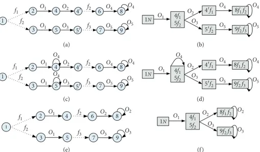
Example 10. Figures 2(a) and 2(b) show two different DESs
and their different diagnosers Gd, Gd, and Gm. We can see
that Gm is isomorphic to the corresponding Gd. Also, note
that in Figure 2(a), two states of Gd, namely, (3N 3f
1) and
(3N 3f2), are merged into one state (3N) in Gm after
minimization. By contrast, in Figure 2(b), two states of Gd,
namely, (4N 5f1) and (4N 6f2), are not merged into one
state (4N) in Gm, as they have different transitions from
themselves (to different states).
According to Definition 4, a number of relevant
prop-erties of minimal diagnoser Gmare given below (which will
be used to prove the subsequent related lemmas/ propositions):
(P1)Let qmi ∈ Qm. For each (qoi, li)∈ qmi , there is at least a state qd
i ∈ Qdin Gdsuch that (qoi, li)∈ qdi.
(P2) Let qm∈ Qm. If (qo, l), (qo′, l′)∈ qm, then there exist s, s′∈ L with se, se′∈ Σo such that T(q0, s) � qo,
T(q0, s′) � qo′, Prj
Σo(s) �PrjΣo(s′), PΣf(s) � l,
PΣ
f(s′) � l′, and either l � l′or l ≺ ≻ l′.
(P3)Let qm∈ Qm. There may exist (qo, l), (qo, l′)∈ qm, that is, the system might reach the same observable state qowith different minimal fault labels (l ≠ l′). (P4)For each qm ∈ Qm and for each (qo, l), (qo′, l′)∈
qm, we have l � l′⟺ l ⊆ l′ l≠ l′⟺ l ≺ ≻ l′ (P5) Let (qmi ⟶ σ qmj)∈ Tm. For each (qo j, lj)∈ qmj, there exists (qo i, li)∈ qmi such that li⊆ lj.
After (offline) building the minimal diagnoser Gm for
DES G and assuming that the current observation is obs, we
can (online) synchronize obs with Gm to reach the
corre-sponding state in Gm to directly obtain the minimal
diag-noses within the state.
Example 11. Consider the DES G outlined in Figure 1(a)
and assume obs � αβθ. According to the minimal diagnoser
Gm outlined in Figure 1(e), we obtain the current minimal
diagnosis N, that is, no fault is produced by (4, N). In addition, when we receive the additional observation c, we
obtain the new minimal diagnosis f 1 (while the
non-minimal diagnosis f 1, f2 in label (10, f 1, f2)of Gd is avoided).
3.3. Minimal Diagnosability of DESs. Just as the classical
diagnosability was defined to determine whether a classical diagnosis has definitely occurred or not, it is natural to define minimal diagnosability to determine whether a set of faults has definitely occurred or not.
In this section, to either strongly or weakly determine whether a set of faults has definitely occurred or not, two notions (strong and weak) of the minimal diagnosability of DESs are proposed.
To introduce the formalizations for the minimal
diag-nosability of a DES G, we define the domain FLto denote
the collection of all possible fault sets of G (with behaviour L) as follows: FL� ∪ s∈L ∧ se∈Σo fi fi∈ s . (15) Obviously, FL� ∪s∈L ∧ se∈ΣoPΣf(s).
3.3.1. Strong Minimal Diagnosability of DESs
Definition 5. A prefix-closed and live language L is said to
be strongly minimally diagnosable if, for any fault set
F∈ FL and for any string s ∈ SF, the following properties
hold: (i) ∀t(t ∈ L/s, te∈ Σo, PΣ f(t)⊆ F) ∃t′(t′∈ L/(st), (tt′)e ∈ Σo, PΣ f(t′)⊆ F)((F ⇝minPrjΣo(st))⟹ D 1 m) (ii) ∃n(n ∈ N) ∀t(t ∈ L/s, te ∈ Σo)(‖t‖≥ n ⟹ ((F ⇝minPrjΣo(st))⟹ D 2 m))
where the strong minimal diagnosability conditions D1
mand
D2
m are defined as follows:
Dm1:ω ∈ Prj−Σ1oPrjΣo stt′⟹ F ≼ P Σf(ω),
Dm2:ω ∈ Prj−Σ1oPrjΣo(st)⟹ F ≼ P Σf(ω).
(16)
In other words, assume that s is a trace in G ending with one fault of F and containing exactly the faulty events of F: (i) For any continuation t of string s without any new fault, the DES will always reach an observable state after a continuation t′ of t (i.e., (tt′)e∈ Σo), also without any new fault, such that if F is a minimal fault set for st, then F will be the unique minimal diagnosis for any trace with the same observation
sequence in stt′ (here, we make an implicit
as-sumption that a faulty event may be triggered by a string many times. In other words, if all faulty events in F have been triggered by string s, then some faults in F may still be triggered again in a suffix string t after s).
(ii) In addition, it is required that there is always a natural number n such that when any continuation t e a b b a 1 0 3 4 5 f3 f1 f2 c g a 0N 0N 0N b c e 3A 5f3 g a b c g e e g c a b c e g (A) DES G (D) Minimal diagnoser Gm (C) Revised diagnoser Gd (B) Classical diagnoser Gd 3N 3f1 5f3 5f1f3 5f3 5f2f3 3N 3f2 3N 5f3 (a) f1 f2 5 0 3 2 a b a 0N a b c e c (A) DES G (C) Minimal diagnoser Gm
(B) Classical diagnoser Gdand revised diagnoser Gd
1 4 7 6 uo c d d e 8 e 9 e b 7N d d e e 0N a b c 4N e 4N c d d e e 4N 5f1 4N 6f2 8f1 9f2 7N 8f1 9f2 (b)
of s is long enough (i.e., the length of t is not less than
n), if F is a minimal fault set for st, then F will be the
unique minimal diagnosis for any trace with the same observation sequence in st.
Note: in contrast with the notion of classical diagnos-ability (Definition 2), here, we add two additional condi-tions, namely, PΣf(t)⊆ F and PΣf(t′) ⊆ F, to restrict later
subsequences, after the complete occurrence of F, such that they do not contain any new fault, except those in F, to ensure that F is still retained as a candidate diagnosis.
In [16], the notion of classical diagnosability is proposed
for checking any single fault fiof G (Definition 2), whereas
our notion of minimal diagnosability is proposed for a set F of faulty events of G, which must be minimal (compared to
other related candidates). Both require that any fault fior
any minimal fault set F must be definitely detected after their occurrences (within a finite delay).
However, there is no logic entailment between the classical diagnosability and our strong minimal diagnos-ability, as shown in the following example.
Example 12. According to Definition 2 and Definition 5,
DES G in Figure 1(a) is strongly minimally diagnosable yet not diagnosable (we can verify the strong minimal diag-nosability of the DES in Figure 1(a) based on Proposition 1 below. That is, we can check the minimal diagnoser in Figure 1(e). It is much easier to find that the minimal diagnoser satisfies the following two conditions in Propo-sition 1: (1) there is no F-indeterminate cycle and (2) there is no F-incomparable state. Thus, the DES in Figure 1(a) is
strongly minimally diagnosable). By contrast, DES G3 in
Figure 3(e) is diagnosable yet not strongly minimally diagnosable.
Before introducing the necessary and sufficient condi-tions for the strong minimal diagnosability of DESs, a number of related definitions and relevant lemmas are provided below.
Definition 6. A state qm ∈ Qm is said to be F-certain if, for any two pairs (qo, l), (qo′, l′)∈ qm (where qo′ can possibly
equal qo), we always have l′� l.
A state qm∈ Qm is said to be F-incomparable if there
exist two pairs (qo, l), (qo′, l′)∈ qm (where qo′ can possibly
equal qo) such that l ≺ ≻ l′.
For instance, the state exactly labelled with 4f 1,5f2in Figure 3 is F-incomparable, whereas other states of minimal diagnosers in Figure 3 are all F-certain. The basic properties of the two types of states are described by the following lemma. Lemma 1. For the minimal diagnoser Gm of DES G, the
following properties hold.
Let Tm(qm
0, s) � qm, s ∈ Σ∗o. If state qmwith fault label l
is F-certain, then for each ω ∈ Prj−1
Σo(s), we have
l≼ PΣf(ω).
If a state qm∈ Qmis F-incomparable, then for any two
pairs (qo, l), (qo′, l′)∈ qm with l ≠ l′, there exist two strings t, t′∈ L with te, te′∈ Σosuch that T(q0, t) � qo,
T(q0, t′) � qo′, PrjΣo(t) �PrjΣo(t′), T
m(qm
0,PrjΣo(t)) �
qm, l � P
Σf(t), l′� PΣf(t′), and l ≺ ≻ l′.
In other words, if a state qmis F-certain, then any trace ω with the same observation projection as observation se-quence s will necessarily contain fault set l. Otherwise, if a
state qm is F-incomparable, then there exist at least two
different traces t and t′ having the same observation
pro-jection but with two incomparable fault sets l and l′.
Definition 7. A set of F-incomparable states qm
1, qm2, . . . ,
qm
n ∈ Qm is said to form an F-indeterminate cycle if
Tm(qm
i ,σi) � qm(i+1) mod n(here, “(i + 1) mod n” represents the modulus of (i + 1) divided by n.), where σi∈ Σo, i ∈ [1 · · · n]. Based on Definition 7, an interesting lemma is given below.
Lemma 2. Assume that qm 1, q m 2, . . ., q m n ∈ Q m are a set of
F-incomparable states forming an F-indeterminate cycle, where qmi � qoi 1, li1 , qoi 2, li2 , . . . , qoi len i, lilen i , qmj � qoj 1, lj1 , qoj 2, lj2 , . . . , qoj len j, ljlen j , (17)
with i, j ∈ [1 · · · n] and len i, len j denoting the number of pairs in qm
i and q m
j, respectively. Then, we have
li1, li2, . . . , lilen i
� lj1, lj2, . . . , ljlen j. (18)
In other words, in an F-indeterminate cycle, any state has the same set of different fault labels. Intuitively, on the one hand, a fault in the current state will stay in the next state (we assume that the faults are persistent); on the other hand, since all states form a cycle, the previous state of the current one can also be seen as the next state. Therefore, all states share the same faults (in fact, Lemma 2 is true for all kinds of cycles. That is, the conclusion is much clearer when all states in the cycle are F-certain). Lemma 3. Given a prefix-closed language L, if F⇝minPrjΣo(s)holds for a fault set F ∈ FLand a string s ∈ L
with se ∈ Σoand PΣf(s) � F, then for any string t ∈ L/s with
te∈ Σoand PΣf(t)⊆ F, we have F ⇝minPrjΣo(st).
In other words, if a fault set F of a trace s is a minimal diagnosis for the observation projection of s, then F is still a minimal diagnosis for any subsequent longer trace from s, provided there is no new fault in the subsequent trace. Lemma 4. Given a prefix-closed language L, F ⇝minPrjΣo(s)
holds for a fault set F ∈ FLand a string s ∈ L with se∈ Σo
and PΣf(s) � F. If F is the unique minimal diagnosis for
observation PrjΣo(s), i.e.,
ω ∈ PrjΣ−1oPrjΣo(s)⟹ F ≼ PΣf(ω), (19)
then for each string t ∈ L/s with te∈ Σo, the following holds:
In other words, if F is the unique minimal diagnosis for a string s (and its projection on the observation is PrjΣo(s)),
then any trace with the same observation PrjΣo(st)will still
contain all the faults in F.
Given the definitions and lemmas introduced above, we now present the necessary and sufficient conditions for the strong minimal diagnosability of a DES G in Proposition 1,
based on its minimal diagnoser Gm.
Proposition 1. A language L generated by an FSM G is
strongly minimally diagnosable iff its minimal diagnoser Gm
satisfies the following two conditions:
(C1)There is no F-indeterminate cycle in Gm
(C2) For each F-incomparable state qm∈ Qm and for
each pair (qo, l)∈ qm, there exist a state qm′ ∈ Qmand a
nonempty observation sequence so∈ Σ +
o such that
Tm(qm, s
o) � qm′, and for each pair (qo′, l′), we have
l′� l, that is, qm′(after qm) is an F-certain state with the
unique minimal fault label l
Remark 3. Condition (C1)is almost identical to the first condition for checking the classical diagnosability in [16], with the exception that “Fi-indeterminate cycle” is replaced
by “F-indeterminate cycle”. However, Condition (C2) is
more complex than the corresponding one for checking the classical diagnosability (where only one statement is needed,
namely, “No state q ∈ qd is ambiguous”), as the strong
minimal diagnosability is conceptually more complex.
Example 13. Consider the three DES models G1, G2, and G3 in Figure 3, where f1, f2, and f3are faults, while the other
events are observable. Their minimal diagnosers Gm
1, G m 2, and Gm3 are also depicted in Figure 3. According to the three
minimal diagnosers, we can find that only G1 is strongly
minimally diagnosable. G2 is not strongly minimally
diag-nosable because it does not fulfil Condition (C1): there does
exist an F-indeterminate cycle including state (4, f 1),
(5, f 2)}and the cyclic transition event o4in G m
2. G3is also not strongly minimally diagnosable because it does not fulfil
Condition (C2): there does exist an F-incomparable state
qm� (4, f 1
), (5, f 2)
in Gm3, but there are no states such
as (4 ′, f 1)or (5 ′, f 2)after qm in Gm 3.
3.3.2. Weak Minimal Diagnosability of DESs. As mentioned
above, according to Definition 5, it is required that any minimal fault set F be the unique minimal diagnosis after a finite delay but before a new faulty event (not in F) occurs. In theory, the condition is very strong. Therefore, we provide the following notion of the weak minimal diagnosability of a DES.
Definition 8. A prefix-closed and live language L is weakly
minimally diagnosable if the following condition holds:
∀F F ∈ FL, ∀s s ∈ SF, ∃n(n ∈ N), ∀t t ∈ L/s, te∈ Σo, t≥ n ⟹ Dm, (21)
where the minimal diagnosability condition Dmis defined in
the following way:
F⇝minPrjΣ o(st) ⟹ ω ∈ Prj−Σ1 oPrjΣo(st)⟹ F ≼ PΣf(ω) . (22) In other words, assume that s is a trace of G ending with a set F of faulty events. For each continuation trace t of s, there always exists a natural number n such that when the length of trace t is greater than or equal to n, and if F is still the minimal fault set for st, then fault set F will be the unique minimal diagnosis for any trace with the same observation projection on st. 6 8 4 2 1 7 9 5 3 5′ 4′ O1 O1 O2 f2 f3 O3 O4 O5 O4 f1 f2 O 5 (a) 8f1 f2 9f2 f3 4f1 1N O2 O4 O5 O4 O5 O1 O3 5′f2 4′f1 5f2 (b) 6 8 4 2 1 7 9 5 3 5′ 4′ O1 O1 O2 f2 f3 O3 f1 f2 O4 O4 O4 O5 O4 O5 (c) 8f1 f2 9f2 f3 1N O1 O4 O4 O5 O4 O5 O2 O3 4′f1 5′f2 4f1 5f2 (d) f2 f3 O2 O3 O2 O3 O1 O1 f1 f2 2 5 7 9 3 4 6 8 (e) 8f1 f2 9f2 f3 1N O1 O2 O3 O2 O3 4f1 5f2 (f )
Figure 3: DES models and minimal diagnosers. (a) DES model G1. (b) Minimal diagnoser G1m for G1. (c) DES model G2. (d) Minimal
diagnoser G2
If the language of a DES has the property of weakly minimal diagnosability, when a trace is long enough (i.e., the length of its continuation t is not less than a given integer n), and if the set of faulty events in the trace is still minimal, then it will definitely be the unique minimal diagnosis. According to the above analysis, the condition of Definition 8 is weaker than that provided in Definition 5 and Definition 2. The following proposition shows the relations between the representation of classical diagnosability and our two rep-resentations of minimal diagnosability.
Proposition 2. Let G be a DES with language L. If L is
strongly minimally diagnosable, then L is also weakly min-imally diagnosable. If L is diagnosable, then L is also weakly minimally diagnosable.
However, based on the following example, we can show that the contrary of Proposition 2 does not hold.
Example 14. According to our definitions, we can see that
DES G3in Figure 3(e) is weakly minimally diagnosable yet not
strongly diagnosable. In contrast, the DES G in Figure 1(a) is weakly minimally diagnosable yet not diagnosable.
Remark 4. The notion of minimal diagnosability allows
missed detection. That is, it is possible that some of the failures are not detected by a minimal diagnoser. For
ex-ample, the occurrence of f2cannot be detected in the DES
model shown in Figure 1(a), although the DES is also weakly minimally diagnosable. After all, only subset-minimal di-agnoses are taken into account in our framework.
In the following, we give the necessary and sufficient conditions for the weak minimal diagnosability of a DES. Proposition 3. A language L generated by an FSM G is
weakly minimally diagnosable iff its minimal diagnoser Gm
does not include any F-indeterminate cycle.
Remark 5. Compared with the necessary and sufficient
conditions for the strong minimal diagnosability of DESs in Proposition 1, the conditions for weak minimal diagnos-ability for the DESs in Proposition 3 are much weaker.
Example 15. Consider the three DESs and the related minimal diagnosers shown in Figure 3. Based on the three
minimal diagnosers, we conclude that both G1 and G3 are
weakly minimally diagnosable. Instead, G2 is not weakly
minimally diagnosable, as there is an F-indeterminate cycle that includes the only state (4, f 1), (5, f 2) and the corresponding cyclic transition event o4in Gm2.
4. Related Work and Comparison
Several works aimed at finding only the minimal diagnosis of DESs are based on either AI planning [43, 44] or SAT ap-proaches [45]. Significantly, they require first to transform a diagnosis problem description into the corresponding knowledge representation, generally with the bottleneck of quickly solving planning or SAT problems for online
diagnosis. However, we generate minimal diagnoses by minimal diagnoser only, which is the main advantage of our approach.
In addition, we compared our method with many other related approaches for diagnosis in different views:
(1) Minimal diagnosis of static systems vs. minimal diagnosis of DESs: Similarity: Like the minimal agnosis of static systems [41, 42], the minimal di-agnosis of DESs is also quite valuable.
(a) First, a diagnosis with fewer faults is more probable than one with more faults
(b) Second, some space is saved by a minimal di-agnosis than corresponding superset diagnoses with very large sizes
Difference: a superset diagnosis of the static system is still a diagnosis, but a superset may not be a diagnosis for a given observation sequence of a DES. (2) Minimal diagnosis vs. diagnosis with probability:
(a) Minimal diagnosis does not need probability information, which sometimes cannot present quite precise diagnoses.
(b) Diagnosis with explicit fault probability based on Bayesian/probabilistic reasoning [32–35] can offer precise diagnoses in a mathematically rig-orous way. However, the shortcomings of these approaches may be twofold.
(i) First, the prior probability of each faulty event is required, which may be difficult to obtain in practice
(ii) Second, adding the probability of each faulty event will possibly make the diagnosis pro-cess more complex
5. Conclusions
In this paper, to focus on the more likely diagnoses, a notion of minimal diagnosis of DESs is proposed, where only subset-minimal fault sets are considered as the most probable explanations for the given observation sequences. Then, the notion of a minimal diagnoser is proposed for the online minimal diagnosis of DESs. Moreover, two sorts of minimal diagnosability are presented for deciding whether a DES is strongly/weakly minimally diagnosable or not, along with necessary and sufficient conditions for testing the minimal diagnosability, which are based on the notion of a minimal diagnoser. Finally, the basic relationships among the three types of diagnosability (classical diagnosability and the two novel notions of minimal diagnosability) are presented.
However, since the generation of the minimal diagnoser requires the availability of the whole DES model, a problem of complexity may arise if the DES is large (which is normal for real, possibly distributed systems). To cope with this problem, as in previous approaches to developing decen-tralized diagnosers, a challenging goal for future research is the decentralization/distribution of minimal diagnoses.