Packet Loss in Terrestrial Wireless and Hybrid Networks

(1)

Packet Loss in Terrestrial

Wireless and Hybrid Networks

Barsocchi Paolo

February 26, 2007

(2)

(3)

Dedications

I would like to thank my advisor Ing. Francesco Potort`ı for his guidance and unlimited support at the professional and personal level during the years that we have been working together. My research would have never reached this level without his contribution.

I would also like to thank the people that cooperated with me to ad-dress some of the research topics: Nedo Celandroni, Erina Ferro and Gabriele Oligeri. I am grateful to all people of Laboratory of Wireless Networks, where I worked these years.

Finally, I would like to thank my family for their permanent support. Especially, I would to express my love to Valentina who has always been there to help me when the work did not progress as expected.

(4)

(5)

List of Figures

2.1 Testbed environment. . . 6

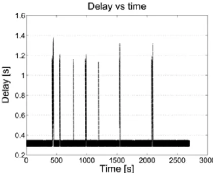
2.2 Typical trend of packet delay for the satellite channel in 45 minutes of transmission. . . 10

2.3 CDF of packet delay for data in 2.2. . . 11

2.4 Details of firsts 40 seconds of 2.2. . . 11

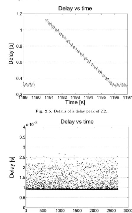
2.5 Details of a delay peak of 2.2. . . 12

2.6 Typical trend of packet delay for the WLAN channel with Retry 0 in 45 minutes of transmission. . . 12

2.7 Lost packets for WLAN transmission with Retry 0 of 2.6. . . 13

2.8 Details of firsts 20 seconds of 2.7. . . 13

2.9 Typical trend of packet delay for the WLAN channel with Retry 7 in 45 minutes of transmission. . . 14

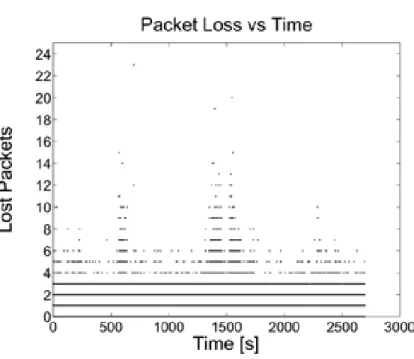
2.10 Lost packets for WLAN transmission with Retry 7 of 2.9. . . 14

2.11 CDF of packet delay for WLAN transmissions. . . 15

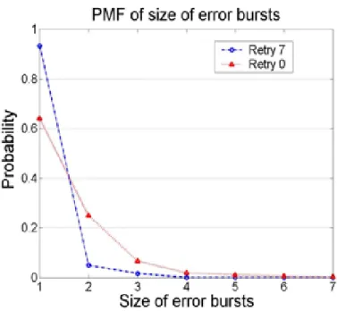
2.12 PMF of the size of packet error bursts for WLAN transmissions. 15 2.13 CDF of packet delay for the WLAN channel with Retry 7, and for the first MAC try only. . . 16

2.14 Packet delay for the full path in 45 minutes of real video streaming. . . 17

2.15 CDF of packet delay for data in Fig. 2.14. . . 17

2.16 Packet jitter for the full path video stream. . . 18

2.17 Lost packets for the full path video stream. . . 18

2.18 The test-bed network topology. . . 21

2.19 Plant of the building. . . 22

2.20 Redundancy and error correction performance vs. coding ratio for client A. . . 23

2.21 Redundancy and error correction performance vs. coding ratio for the client B. . . 24

2.22 MOS of received video by client A. . . 26

2.23 Samples of the streamed video trailer at different coding and bit rates. . . 27

(10)

3.1 A typical scenario of mobile radio communications . . . 31

3.2 Angle of arrival of the nth _{incident wave . . . 32}

3.3 Channel fading types . . . 34

3.4 Small-scale fading (grey line) and large-scale fading (black line) 35 3.5 Path loss vs. distance measured in several German cities [7] . . . . 37

3.6 Flat-fading case: Bs is the signal bandwidth, and Bc is the coherence bandwidth . . . 39

3.7 Flat-fading channel characteristics . . . 39

3.8 Frequency selective fading case: Bs is the signal bandwidth, and Bc is the coherence bandwidth . . . 40

3.9 Frequency selective fading channel characteristics . . . 41

3.10 Type of small fading . . . 42

3.11 Type of small-scale fading types of experienced by a signal from the viewpoint of (a) symbol period, (b) baseband signal bandwidth. . . 43

3.12 Types of small-scale fading for the IEEE802.11 signal . . . 44

3.13 Maximum excess delay . . . 46

4.1 2-ray ground reflection model. . . 54

5.1 Channel model based on a two-state Markov chain. . . 66

5.2 Error gap distribution for the Gilbert model. . . 67

5.3 Error bursts distribution for the Gilbert model. . . 68

6.1 Error of packet intervals at the receiver. . . 76

6.2 Transmitted frame. . . 77

7.1 Comparison between 2-ray propagation models at Wi-Fi and GSM frequencies for ht= hr = 1 m. . . 82

7.2 Measured signal level, double regression model and two-ray model with sensitivity thresholds for ∆L = 0. Error bars indicate 0.05, 0.50 and 0.95 quantiles of observed values. . . 83

7.3 Horizontal radiation pattern for two PCMCIA cards (vertical polarisation). . . 84

7.4 Frame errors and signal levels for each transmission rate. . . 86

7.5 Probability mass function of burst lengths. . . 87

7.6 Probability mass function of gaps lengths. . . 88

7.7 Chi-square test results. . . 89

7.8 Fit of Equation 7.10 with measured values. . . 90

8.1 Plant of the building where the measurements have been taken; T and R are the transmitter and receiver laptops used for the measurements. . . 96

8.2 Average of received, lost and corrupted frames during the first week. . . 97

(11)

List of Figures XIII

8.3 Average of received, lost and corrupted frames during the

second week. . . 97

8.4 Average of received, lost and corrupted frames during the third week. . . 98

8.5 Probability mass function of burst length at frame level. . . 99

8.6 Probability mass function of gap length at frame level. . . 99

8.7 Probability mass function of gap length at bit level. . . 100

8.8 Probability mass function of burst length at bit level. . . 101

8.9 Probability mass function of number of errored bits per frame . . 102

9.1 Plant of the building where the measurements have been taken; T and R are the transmitter and receiver laptops used for the measurements. . . 107

9.2 Error gap length distributions for one observed frame error trace and a synthetically generated Bernoulli trace with the same average frame error rate. . . 109

9.3 Goodput as computed with Padhie’s formula and with a trace with Bernoullian frame error. . . 110

9.4 TCP goodput versus frame error rate of real traces for different error models. . . 111

(12)

(13)

List of Tables

2.1 Packet loss, packet delay and packet jitter statistics of the satellite and WLAN transmissions, relative to 45 minutes of CBR traffic presented in Fig. 2, 6 and 9. . . 9 2.2 Statistics of the full path transmission, relative to 45 minutes

of a real video streaming. . . 19 2.3 Maximum, mean and variance of delivery delay for client A. . . . 25 2.4 Maximum, mean and variance of delivery delay for client B. . . . 25 2.5 Acceptability of received video by client A. . . 25 3.1 Path loss exponents for different environments. . . 36 3.2 Typical values of mean delay spread and maximum delay spread. 45 4.1 Characteristics of the considered outdoor propagation models. . 56 7.1 Rate-dependent parameters in Equation 7.10. . . 91 9.1 Traces used in the simulation experiment. . . 111

(14)

(15)

1 Introduction

The presence of both a geostationary satellite link and a terrestrial local wire-less link on the same path of a given network connection is becoming increas-ingly common, thanks to the popularity of the IEEE 802.11 protocol [1]. In the following, we will refer to this ubiquitous wireless terrestrial protocol as Wi-Fi, the popular trademark of the association founded to set interoper-ability standards for it. The most common situation where a hybrid network comes into play is having a Wi-Fi link at the network edge and the satel-lite link somewhere in the network core. Example of scenarios where this can happen are ships or airplanes where Internet connection on board is provided through a Wi-Fi access point and a satellite link with a geostationary satel-lite; a small office located in remote or isolated area without cabled Internet access; a rescue team using a mobile ad hoc Wi-Fi network connected to the Internet or to a command centre through a mobile gateway using a satellite link [2, 3]. The serialisation of terrestrial and satellite wireless links is prob-lematic from the point of view of a number of applications, be they based on video streaming, interactive audio or TCP. The reason is the combination of high latency, caused by the geostationary satellite link, and frequent, corre-lated packet losses caused by the local wireless terrestrial link. In fact, GEO satellites are placed in equatorial orbit at 36,000 km altitude, which takes the radio signal about 250 ms to travel up and down. Satellite systems exhibit low packet loss most of the time, with typical project constraints of 10−₈ bit error rate 99% of the time, which translates into a packet error rate of 10−_{4, except for a few days a year. Wi-Fi links, on the other hand, have quite} different characteristics. While the delay introduced by the MAC level is in the order of the milliseconds, and is consequently too small to affect most applications, its packet loss characteristics are generally far from negligible. In fact, multipath fading, interference and collisions affect most environments, causing correlated packet losses: this means that often more than one packet at a time is lost for a single fading event [3].

In chapter 2 we describe the hybrid wireless network; in fact natural and man-made disasters, like earthquakes, floods, storms, structural collapses, etc.,

(16)

pose a challenge to public emergency services. In order to cope with such disasters in a fast and coordinated manner, communications between rescue squads, both among themselves and outside the assisted zone, play a critical role. This chapter is subdivided in two main section; in section 2.1 we evalu-ated the performance in terms of packet loss, delay and jitter for the satellite path, wireless path and finally for the full path, while in section 2.2 we study how to improve the QoS (Quality of Service) requirements of the multimedia flows. This portion of the study offers an subjective assessment of video qual-ity as a function of channel error characteristics, together with explanations for the performance degradations based on network-level effects.

From a user’s perspective, the details of the wireless technology used are generally unimportant: it’s the performance of the final wireless-based ap-plication that counts. We distinguish two basic types of user apap-plications: real-time datagram applications, with various quality of service constraints, and TCP-based applications, whose main performance indicator is the con-nection throughput. Analysing the performance of these applications on a wireless channel is challenging, because of the highly variable characteristics of the channel and the number of different causes that influence them. The aim of this dissertation is to analyse the behaviour of a wireless channel at the packet level in order to build a model able to capture the channel’s main char-acteristics. In order to validate this model, we will resort to simulation and real-world measurements. A good knowledge of physical layer and the funda-mental limitations in the performance of mobile communications system are necessary tools for engineers as well as for research scientists that wish to gain to a deeper understanding of a possible channel modelling. Therefore, in chap-ter 3 we describe a typical scenario for chap-terrestrial mobile radio channel and the principal cause of the information loss (multipath fading). In fact, multipath propagation caused by reflections and the scattering of radio waves lead to a situation in which the signal phase is shifted depending on the length of each of the paths between transmitter and receiver, where signals carried over differ-ent paths are superimposed. This interference can strengthen, distort or even eliminate the received signal. Conditions that cause fading are illustrated in the third chapter. We will examine the fading effects that characterize mobile communications: large-scale fading and small-scale fading. Large-scale fading represents the average signal power attenuation, also called path loss, due to motion over large areas, while the small-scale fading refers to the sometimes dramatic changes in signal amplitude and phase that can be experienced as the result of small changes in the spatial separation between receiver and transmitter.

Knowledge of the properties of the time-varying frequency and space dis-persive mobile radio channel is necessary for a good understanding of the phenomena that occur in wireless communications and for the design of mo-bile communication systems and networks. In chapter 4, an overview of state of the art in the modeling of the mobile radio channel is given.

(17)

1 Introduction 3

Channel models are of particular interest for radio communication systems and network technologies like UMTS (Universal Mobile Telecommunications System) and WLAN (Wireless Local Area Networks). Thus, this work fo-cuses on mobile terrestrial channel modelling, in general, and, in particular, on the modeling of radio wave propagation in urban and suburban areas. We will investigate the propagation models that characterize signal strength over large transmitter-receiver separation distances (large-scale propagations mod-els) and models that characterize the rapid fluctuations of the received signal strength over short distances (small-scale models), both in outdoor and indoor scenarios. Chapter 4 is divided in two main sections: Section 4.1 addresses the outdoor models, while Section 4.2 focuses on the indoor models.

In Chapter 5, we describe the traditional approach to modelling packet losses through the use of a classical network model, such as Bernoulli, Gilbert-Elliot. In order to choose the best model, we must consider the statistical properties of them. For example, the Bernoulli model is based on a memoryless process. Thus, output values will be uncorrelated.

In Chapter 6, we will describe a complex and articulated campaign of measurements, together with tools used to generate and analyze the data. The campaign of measurements is conducted in outdoor and in indoor envi-ronments. The packet loss and the throughput are directly measured using a traffic generator and a receiver inserted at MAC layer.

Our goal would be to obtain a certain number of models, derived from real measurements, according to the environment characteristics; this argument is dealt in chapter 7 for the outdoor model.

In chapter 8 we describe the results obtained during the indoor measure-ment campaign, with are especially focused on burst length and gap length distributions. This chapter is subdivided in two main section; Section 8.1 ad-dress the main frame level statistics, while section 8.2 focuses on presents the results obtained at bit level.

Finally in chapter 9 we concentrate on frame error models in indoor en-vironment targeted to TCP-based applications, for which the combination of high, correlated packet loss and high latency may cause very bad performance. Since TCP interprets packet loss as a sign of congestion, thus slowing its pace to avoid worsening the network conditions, frame errors due to corruption causes decreased throughput, even in the absence of network congestion.

(18)

(19)

References

1. IEEE Std 802.15.1-2002 IEEE Std 802.15.1 IEEE Standard for Information tech-nology - Telecommunications and information exchange between systems - Lo-cal and metropolitan area networks - Specific requirements Part 15.1: Wireless Medium Access Control (MAC) and Physical Layer (PHY) Specifications for Wireless Personal Area Networks (WPANs).

2. A. Annese, P. Barsocchi, N. Celandroni, and E. Ferro, “Performance evaluation of UDP multimedia traffic flows in satellite-WLAN integrated paths”, proceedings of 11th Ka Band Utilization Conference, Rome, September 2005.

3. F. Davoli, E. Ferro, H. Mouftah, “Wireless access to the global Internet: mobile radio networks and satellite systems”, guest editorial, Int. Journal of Communi-cation Systems, vol. 16, no. 1, 2003.

4. Gabriele Oligeri, “Misura e caratterizzazione di un canale Wi-Fi”, http://fly. isti.cnr.it/didattica/tesi/Oligeri-Finotti/Oligeri.pdf.

(20)

(21)

2 Hybrid network

Natural and man-made disasters, like earthquakes, floods, storms, structural collapses, etc., pose a challenge to public emergency services. In order to cope with such disasters in a fast and coordinated manner, communications be-tween rescue squads, both among themselves and outside the assisted zone, play a critical role. In the hours and even days following these events, commu-nication is often limited, due to the damages caused by the disaster to land connections or because the event occurred in an area without infrastructures. Wireless communications are the reply to these needs; wireless networks are the easy, fast, and intuitive way for providing the first communications means for the depicted scenarios. In particular, MANET (Mobile Ad hoc NETworks) [1] is the topology generally contemplated in these situations, in which handheld devices or notebooks use wireless ad-hoc networks for com-munications between each other and with a special node, which is a gateway for outside communications, through a satellite link.

Given such a network, we assume that user data are flows derived from multimedia and real-time applications, like voice calls, video streaming, and video conferencing, which make use of UDP (User Datagram Protocol) trans-port protocol.

2.1 Performance evaluation

In this chapter, we present a set of experimental results, which show the be-haviour of UDP traffic flows in a basic MANET testbed developed at ISTI. The testbed is constituted by a set of portable computers and handsets, in-terconnected among them in wireless mode, and a Skyplex Data satellite link [2, 5]. The portable computer that acts as a gateway between the ad-hoc net-work and the Skyplex box is a Debian Linux box (kernel 2.6.8, Celeron 1.133 GHz with 256 MB of RAM).

Wireless LANs [6, 7] have the advantage of low delivery delays, but they have drawbacks such as the high channel errors due to multiple paths and

(22)

data collisions. Satellite links have an inherent broadcast facility, but they suffer from high delivery delays and atmospheric adverse conditions which may worsen the Signal to Noise Ratio (SNR). Thus, the whole network, made up of WLAN nodes and the satellite link, is not a trivial environment for QoS (Quality of Service) requirements of the multimedia flows.

The packet loss, the data jitter and delay are separately measured in both the WLAN and the satellite link; then, these three parameters are evaluated as total, combined effects on the hybrid wireless network considered. The traffic flows used are both a simple CBR (Constant Bit Rate) generator, character-ized by the size of the IP datagram packets and the packet generation time interval, and a multimedia and real-world video application. The investigation aims at evaluating the QoS performance of traffic flows, both in unicast and in broadcast/multicast transmission mode. Delivery delays, from the application layer’s point of view, are finally calculated, which are useful for estimating the buffer’s sizes of the receiving applications.

2.1.1 Testbed configuration

The testbed of transmission experiments is depicted in 9.1.

Fig. 2.1. Testbed environment.

The wireless path at ISTI is made up of notebooks (Celeron 1.133 GHz with 256 MB of RAM) equipped with a Debian Linux operating system (ker-nel 2.6.8) and with wireless PCMCIA network cards of different manufactur-ers (CNet CNWLC-811 IEEE802.11b for transmission, Conceptronic C54RC IEEE802.11g for reception), always operating with the standard DCF (Dis-tributed Contention Function) [7] contention access mode at a rate of 11 Mbps,

(23)

2.1 Performance evaluation 9

and acting as traffic sources. An host acts as a gateway between the WLAN network and the Skyplex box, and forwards packets towards the satellite.

The satellite link is a Ka channel of Eutelsat HotBird 6 which uses the technology known as Skyplex Data [2, 3, 5]. This is an IP-based satellite network derived from the DVB-RCS [4] and it is used here in a standard point-to-point (for unicast traffic) and point-to-multi-point (for multicast traffic) topology.

We have used remote Linux hosts in Bari and in Genoa as traffic sinks on the other side of the satellite link.

In unicast transmissions, WLAN cards use standard IEEE802.11 settings; in particular, the DCF Retry Limit value is set to 7 for every outgoing MAC frame, i.e. up to 7 transmission retries are performed in case of unacknowl-edged frames. In multicast transmissions, the value of the Retry Limit is 0, i.e. the frame is transmitted only one time, regardless its good reception. 2.1.2 The Measurements

In the first step, UDP packets have been transmitted through a simple CBR generator written in C, in order to testing the single WLAN or satellite links and investigating their basic performance; about 24 hours of measures has been performed both on the satellite channel and on the WLAN channel, with single tests of 45 minutes each; then a real-world MPEG-4 video stream has been transmitted with the software VLC (Video Lan Client) on the full WLAN and satellite path.

A software in C has been developed with the purpose of tracking and collecting packets in the cardinal points of the path, i.e. at the WLAN source, the satellite gateway and the remote sink. This software runs on Linux in user mode, so the collected statistics refer to the application’s layer; all the time measures (the end-to-end jitter and delay) have the precision of the Linux kernel clock. The gettimeofday() system call has been used; it returns microseconds-figure time from the Linux System Time.

We have gathered our measurements with notebooks located in fixed in-door positions at about 10 meters apart from the satellite gateway, separated by thin walls and doors, and with people working around involved in the common activities of an office environment.

Several measurement campaigns have been carried out, with CBR traffic at different transmission rates, varying both the packet lengths and their inter-generation time. It is well known that WLAN communication’s performances widely change according to environment, people’s presence and movements; thus, we here present only the most representative tests of the common sit-uation observed, and we introduce a way for deriving Retry 0 transmission performances from the Retry 7 ones, so that a direct comparison is possible between the two WLAN operating modes.

Every test presented in this work lasts 45 minutes; every packet generated has its own sequence number; for all packets that travel through the three

(24)

cardinal points of observation of the network, the software sniffs pieces of information like the sequence number, the packet length and the transit time. Each packet may experience a different transmission delay, so a jitter, defined as the difference between two transmission delays, is induced on the packet arrival time [8, 9]. By definition, in every single hop, the first packet received has a null jitter, while the nth packet (transmitted at the time tT X,n and received at the time tRX,n) has the jitter jn,1given by

jn,1= (tRX,n− tRX,1) − (tT X,n− tT X,1) (2.1) i.e. the jitter jn,1 is referred to the transmission delay of the first packet, because this is comfortable for the delay calculation.

Since it’s difficult to synchronize the clocks of the observation points and every clock has its own drift, we assumed linear clocks’ drift. A linear correc-tion has thus been adopted along with every interval of 12 consecutive hours of measures. In short, the slope of the linear part of the jitter drift, caused by the different clock drift of the transmitting and receiving side, has been calcu-lated for such intervals, and a linear correction proportional to the time was applied at every jn,1. Then, an offset O is added to the jitters so calculated in order to obtain the packet delays Dn given by

Dn = jn,1+ O Dhop= min {Dn} (2.2)

so that the minimum delay obtained is equal to the minimum delay of the hop Dhop, measured as the half of the minimum round trip time of 1000 ping packets sent with the same size and inter-generation time of the analyzed packets.

Furthermore, continuous jitter calculation, as specified by RTP protocol in [10], is evaluated as

Jn= Jn−1+|jn,n−1| − Jn−1

16 (2.3)

where the difference between transmission delays jn,n−1is referred to con-secutive packets. From this point, when we speak of packet jitter, we are referring to this Jn.

The satellite path

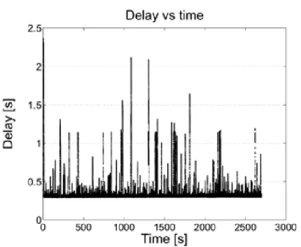
Fig. 2.2 shows the packet delay of the typical satellite transmission test, for a CBR traffic with UDP packets of 1000 bytes (IP header included) and packet inter-generation time of 20 ms, following a generated rate of 400 kbps. The figure shows a packet delay quite regular and concentrated, except for rare peaks, in which the system seems to recover after a sort of bad situation. It is worth pointing out that the satellite used performs on board processing, and is shared in TDMA (Time Division Multiple Access) mode with other users. Fig. 2.4 and 2.5 show the details of the regular band and of the peaks

(25)

of the packet delay, respectively. In particular Fig. 2.5 shows what’s happens when, for a less then 1 second time interval, packets are not transmitted in the satellite path: when transmission resumes the delay has piled up but the situation restores in about 5 seconds. This phenomenon has been observed in all the satellite transmission tests and the recovery speed is due to the channel available bandwidth, that is 2 Mbps. Fig. 2.3 presents the CDF (Cumulative Distribution Function) for the packet delay.

The satellite channel has resulted to be almost error-free; very few losses have been observed so that is not possible to give a precision value of the packet loss. No single packet errors have been registered and this is probably due to the peculiarity of Skyplex architecture; error bursts of 2 or 3 consecutive packets have rather been seen.

The minimum delay measured on the satellite path has been 0.284619 s; table 2.1 shows the mean and standard deviation of the packet delay and the mean packet jitter.

Table 2.1. Packet loss, packet delay and packet jitter statistics of the satellite and WLAN transmissions, relative to 45 minutes of CBR traffic presented in Fig. 2, 6 and 9.

Packet loss Packet delay [s] Mean jitter [s] probability Mean Standard

deviation Satellite - 0.334329 0.104579 0.0133456 WLAN Retry 0 3.33 · 10−1 _0.000912 _0.000094 _0.000028 WLAN Retry 7 4.82 · 10−4 _0.001379 _0.001080 _0.000669 WLAN “Retry 0” emulated 2.12 · 10 −1 _0.000978 _0.000091 _0.000022

The WLAN path

Fig. 2.6 shows the packet delay of the typical WLAN transmission test with Retry 0 (suitable for multicast and broadcast transmission), for a CBR traffic with UDP packets of 1000 bytes and packet inter-generation time of 20 ms. The delay is quite constant and delimited within a narrow band. Fig. 2.7 and 2.8 show the size of packet error bursts during the test. The packet loss, the mean packet delay, its standard deviation and the mean packet jitter for this test are shown in table 2.1.

Fig. 2.9 shows the packet delay of a WLAN transmission test like the previous one, but with Retry 7 (suitable for unicast transmission). It’s plain that the different bands in which the delays of the packets are gathered cor-respond with the retries the WLAN MAC layer operates. As shown in table 2.1, the mean and standard deviation of packet delay for WLAN Retry 7 test is greater then the WLAN Retry 0, but the packet loss benefits of the retries. This is plain visible in Fig. 2.10, that shows the size of packet error bursts

(26)

for the Retry 7 test, and in Fig. 2.12, that show a comparison of the PMF (Probability Mass Function) of the size of packet error bursts for the Retry 0 and Retry 7 tests. In Fig.2.11 the CDF for the packet delay of Retry 0 and Retry 7 tests are compared.

Fig. 2.2. Typical trend of packet delay for the satellite channel in 45 minutes of transmission.

It’s important to notice that WLAN channel’s performances widely change due to radio multipaths and environment variations, and the two WLAN tests shown before are not really comparable. In fact in other Retry 7 tests very heavy packet losses have been found too.

Instead it’s easy to discriminate for the most part of the packets of the Retry 7 test, the ones received at the first MAC try from that received at subsequent retries, simply watching the delay accused by each packet. If the Retry would be set to 0 all packets transmitted with MAC retries would have been lost. So it’s possible for the Retry 7 test to go back and to achieve roughly what’s would be happened in the same situation if the Retry would be set to 0. Fig. 2.13 show the CDF of packet delay for the WLAN channel with Retry 7 compared to the one obtained for the first MAC try only of the same transmission (for the purpose packets with delay less or equal to 0.0026s have been considered first MAC try packets). Table 2.1 show the packet loss, the mean packet delay, its standard deviation and the mean packet jitter for this comparable “Retry 0” emulated transmission.

(27)

Fig. 2.3. CDF of packet delay for data in 2.2.

(28)

Fig. 2.5. Details of a delay peak of 2.2.

Fig. 2.6. Typical trend of packet delay for the WLAN channel with Retry 0 in 45 minutes of transmission.

(29)

Fig. 2.7. Lost packets for WLAN transmission with Retry 0 of 2.6.

(30)

Fig. 2.9. Typical trend of packet delay for the WLAN channel with Retry 7 in 45 minutes of transmission.

(31)

Fig. 2.11. CDF of packet delay for WLAN transmissions.

(32)

Fig. 2.13. CDF of packet delay for the WLAN channel with Retry 7, and for the first MAC try only.

The minimum delay measured on the WLAN path has been 0.000883s. Full path behaviour

A transmission of a real MPEG-4 video stream has been performed over the full WLAN and satellite path. The software VLC [11] has been used as source: it generates UDP packets of a fixed size of 1344 bytes (IP header included) with a variable inter-generation time. Further 4 bytes has been added to each of that packets, for tracking purposes. The transmission has lasted 45 min-utes, and 160402 packets has been generated, achieving a mean throughput of 640.7 kbps. The WLAN hop has operated in the Retry 0 mode, emulating a multicast or broadcast transmission, within a quite clear channel.

Table 2.2 shows the packet loss, the mean packet delay, its standard de-viation and the smoothed mean jitter measured in each hop, and the ones resulted in the total full path.

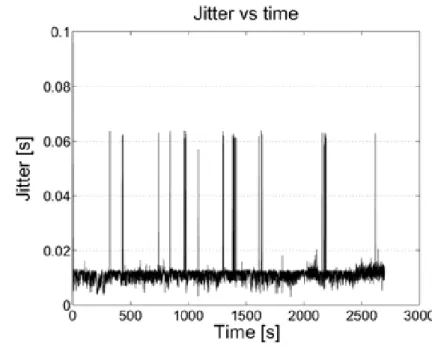
Fig. 2.14, 2.15 and 2.16 show the trend of the packet delay, the CDF of the packet delay, and the packet jitter, for the full path streaming, respectively. Most of that are due to the satellite hop. Fig. 2.17 shows the lost packets in the full path, but they are fully due to the WLAN hop.

(33)

Fig. 2.14. Packet delay for the full path in 45 minutes of real video streaming.

(34)

Fig. 2.16. Packet jitter for the full path video stream.

(35)

2.2 Forward Erasure Correction and Real Video Streaming 21 Table 2.2. Statistics of the full path transmission, relative to 45 minutes of a real video streaming.

Packet loss Packet delay [s] Mean jitter [s] probability Mean Standard

deviation

WLAN (Retry 0) 4 · 10−2 _0.000940 _0.000231 _0.000021 Satellite - 0.367103 0.196004 0.010863 Full path 4 · 10−2 _0.367946 _0.196004 _0.010864

2.1.3 Conclusions

A WLAN cum satellite testbed has been developed, and UDP transmissions have been performed both with CBR traffic and with a real video stream. The packet loss, the packet delay and the packet jitter have been experimented.

In the end the resulting packet loss of this hybrid network topology is fully due to the losses in the WLAN hops, while most of the delay and the jitter comes from the satellite hop.

The Quality of Service of multimedia and real-time transmissions over this kind of network topology is severely tried, and the negative effects of each hop are summed in the full path.

A buffer of few seconds located at the receive application, according to the experimental results found, could assure the quality of multimedia non real-time streams. It would be better to implement in the WLAN hops a stronger loss recovery strategy, because the Retry 7 mode improve the safety of trans-mitted packets but it’s not suitable for multicast and broadcast transmissions. Adaptive Forward Error Correction (FEC) techniques could be used instead in the WLAN hops: they could improve the packet safety with the trade-off of a little increase of the delivery time of the packets. This topic could be investigated in future research. Nothing could be done for the minimum delay introduced by the satellite channel, and this could be the biggest problem for real-time interactive applications.

The investigation of TCP flows within the hybrid topology described is another interesting topic: the optimization of the goodput of TCP flows is a challenging problem to be investigated as well; this issue is currently argument of ongoing research.

2.2 Forward Erasure Correction and Real Video

Streaming

In a heterogeneous MANET, based on wireless LANs linked together by via satellite, the overall channel efficiency is impaired by multiple effects, because of multipath fading in the terrestrial segment and atmospheric fading on the satellite link. In this paper, we address this issue by applying forward erasure

(36)

correction codes (FZC) to MPEG-4 video sequences exchanged by the hosts of a hybrid network, . The network is made of a satellite link and a wireless LAN that uses 802.11b devices. The stream is FZC encoded at the streamer and decoded at the individual receivers. Encoding and decoding operations occur just above the transport layer. This approach has the advantage of being independent of the equipment, the operating system and the end-user appli-cation. It performing performs as middleware between the application and the underlying operating system services, and thus allows allowing the employing use of standard streaming applications both at the sender and the receiver. This work aims at demonstrating the improvement in quality of service of the video transmitted in the hybrid network. The main parameters measured are the packet loss, the delivery delay, and the overhead in bandwidth occupancy imposed by the use of FZC. The received video is then evaluated by using a MOS (Mean Opinion Score) procedure. While the concept of using FZC has been widely studied for several years [12, 13], the literature is lacking in ex-perimental results in a hybrid wireless environment. In the following, we first describe our test scenario and then we present measurements obtained in the described environment.

2.2.1 The Real Case Study

The forward error correction technique employed in our experiments a class of linear block codes based on Vandermonde matrices [14]. Basically, k blocks of source data are encoded to produce n blocks of encoded data, such that any subset of k encoded blocks suffices to reconstruct all source data (with n > k). Let x be the vector of source blocks and y the vector of encoded blocks. Then, the problem is to find an appropriate nk coding matrix C such that y = Cx and x = C0−1_y0_{, for any subset y}0 _{of k blocks in y, where C}0 is the corresponding row-wise sub-matrix in C (a linear block code is said to be systematic if I is a row-wise sub-matrix in C). As indicated in [14], of special interest are the FZCs derived from Vandermonde coding matrices are of special interest; they employ efficient field arithmetic.

The video stream used in the experiment is coded using 4. MPEG-4 is the first standard that describes multimedia contents as a set of audio-visual objects to be presented, manipulated and transported individually. The high compression ratio and error resilience offered by MPEG-4 has driven an explosion of its popularity. The evaluation of FZC performance in MPEG-4 stream delivery on the single wireless path is not new. For example, in [15] the joint usage of FZCs and MPEG-4’s Fine Granularity Scalability (FGS) – a highly suitable technique for IEEE 802.11 –is studied, while [16] studies the behavior of FZCs when applied to MPEG-4 streaming via 3G networks. Anyway, there is a lack of experimental results in hybrid wireless environment. In order to provide such results, our target scenario is composed of a video-streaming server interconnected to an ad hoc wireless network through an OBP (On Board Processing) satellite. The satellite link is carried by the

(37)

2.2 Forward Erasure Correction and Real Video Streaming 23

Eutelsat HotBird6 satellite in Ka band, and uses the technology known as Skyplex Data [5, 6], which is, an IP-based satellite network, derived from DVB-RCS. We used it this satellite technology in a point-to-multipoint topology, by using a single multicast receiver. The Skyplex link we used has a bandwidth of 2 Mb/s. Figure 2.18 depicts the scenario of our experiment. The video streamer transmits a FZC encoded multicast stream on the satellite; the local gateway receives the traffic from the satellite multicast receiver and broadcasts forwards it to the wireless clients. The ad-hoc wireless LAN uses the IEEE 802.11b standard [5].

Fig. 2.18. The test-bed network topology.

The mobile devices are IBM Thinkpad R40e laptops (Celeron 2.0 Ghz with 256 Mb Ram running Debian Linux with a 2.6.8 kernel), and they are equipped with CNet CNWLC-811 IEEE 802.11b wireless cards. The indoor environment is depicted in Fig. 2.19

The dashed lines in Figure 2.19 represent the shortest radio paths between the local gateway and the client devices A and B (black stars). The rooms are at the first floor of the building of the CNR ISTI Institute in Pisa; they are delimited by thin walls.

2.2.2 Experimental Results

Notice that IEEE 802.11 includes the use of automatic repeat request (ARQ) [5] only in unicast mode. We implemented two software modules, an encoder

(38)

Fig. 2.19. Plant of the building.

and a decoder, written in C language, by using Rizzo’s library [18]. The en-coder works at the transport layer by fetching blocks of k information packets from the video stream and then transmitting k +l UDP packets (k of informa-tion + l of redundancy) towards the receiving host. At the receiving host, the decoder fetches k of the k + l packets per block and recovers the information, provided that no more than l packets are lost in a single block of packets. The receiver then feeds the VLC 0.8.1 decoder with the received stream to the VLC 0.8.1 decoder with the received stream. VLC uses a packet size of 1316 bytes, which is a block of seven 7 MPEG-4 frames. The encoder adds a preamble of 4 bytes for the sequence number, which is then cancelled by the decoder. The overall length of the 802.11 MSDU is then equal to 8+20+8+4+1316 bytes, keeping into account the UDP, IP, and SNAP/LLC headers.

Packet error rate

The MPEG stream carries an Xvid version of the Pirates of Caribbean movie, with a frame rate of 25 frames per second at 576320 pixels, and an average data stream of 939 kb/s. Our experiments show that the satellite channel is error free (thus the only problem is the intrinsic satellite delay), while the wireless channel is error prone. Thus, the error recovery aspect must be addressed in the wireless environment. By default, 802.11 devices use an internal algorithm for changing the transmission signal rate in order to adapt to varying channel conditions. Since our aim is to verify the performance of different coding schemes, we fixed the signal rate, by disabling the internal auto rate-change algorithm. We used two data bit rates: 11 and 5.5 Mb/s. Lower transmission rates were not considered because the stream throughput would have exceeded the available information rate of the wireless channel. We analyze the channel between the local gateway and the A node (see Fig. 2.19), and between the local gateway and the B node (see Fig. 2.19), respectively. In the first case, which is the worst case (due to the distance between the gateway and the

(39)

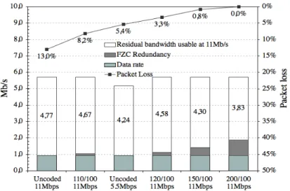
client A), the experiment in uncoded mode (no FZC) shows that packet loss can be reduced from 13% to about 6% by changing the transmission rate from 11 to 5.5 Mb/s. In this case, the channel occupancy increases by 56%. A similar redundancy is required when using an FZC coding ratio of 150/100; however, in the latter case, we measured a much better performance, with a packet loss rate of 0.8%. Better performance yet can be obtained by using an FZC with 120/100 coding ratio, which increases channel occupancy by only 20%.

Fig. 2.20. Redundancy and error correction performance vs. coding ratio for client A.

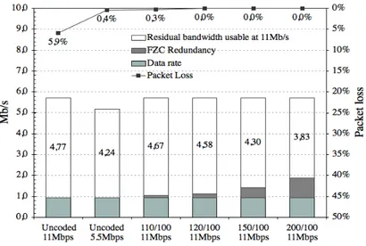
When the B node is considered, the experiment in uncoded case (no FZC) shows that packet loss can be reduced from 5.9% to about 0.4% by changing the transmission rate from 11 to 5.5 Mb/s. However, if we use an FZC coding ratio of 110/100, we measured a much better performance (only 0.3% of packet loss) by increasing the channel occupancy by only 10%. Choosing a coding ratio of 120/100, all packet losses (about 6%) can be recovered by increasing the channel occupancy by 20%.

All measurements are summarized in Figures 2.20 and 2.21, where the residual bandwidth is defined as the bandwidth left available on the channel for use by other communications performed at 11 Mb/s. Notice the case of 5.5 Mb/s where, while no FZC redundancy is introduced, the occupied channel

(40)

share is 56% wider than the corresponding 11 Mb/s case, and the residual bandwidth is reduced accordingly.

Generally speaking, there is a tradeoff between redundancy and error cor-rection performance; these results show that the usage of FZC is convenient with respect to changing the signal rate.

Fig. 2.21. Redundancy and error correction performance vs. coding ratio for the client B.

Packet delivery delay

A streaming application delivers time-based information, i.e. user data that has an intrinsic time component. By using erasure codes we introduce the packet delivery delay. In fact, when h packets in a block are lost, we must wait for all k packets of information plus h of redundancy. Delivery delay is an important parameter that must be evaluated like the packet loss. Our experiments show that the mean delivery delay for the node A is about 50 ms, and it is less than the delivery delay for the node B (48 ms). This is due to the fact that node A has a greater number of packet losses than node B. The maximum packet delivery delay is evaluated as the time necessary to recovery all the information when a number of packet equal to the redundancy packets is lost. These experiments show that the limits imposed by ITU-T Recommendation G.114 [18] are preserved. Tables 2.3 and 2.4 show the packet delivery delay for clients A and B, respectively.

(41)

2.2 Forward Erasure Correction and Real Video Streaming 27 Table 2.3. Maximum, mean and variance of delivery delay for client A.

Coding ratio Max [ms] Mean [ms] Var. [ms] 110/100 105.6 52.149 0.769 120/100 115.2 54.99 0.792 130/100 124.8 52.637 0.805 200/100 192 53.805 1.675

Table 2.4. Maximum, mean and variance of delivery delay for client B. Coding ratio Max [ms] Mean [ms] Var. [ms]

110/100 105.6 48.522 0.796 120/100 115.2 48.639 0.824 130/100 124.8 47.992 0.715 200/100 192 53.585 1.681

Mean opinion Score (MOS)

The MOS is the most widely known video quality metric. MOS is a subjective score, ranging from 5 (Excellent) down to 0 (Unacceptable). Thirty persons have answered to three quality questions (overall, video, and audio quality) for each coding ratio of the video received by client A; mean opinion scores have been calculated. The results for each quality question are shown in Figure 2.22. It can be seen that the coding ratio is important for opinions on the quality; this is true for all three questions. Not surprisingly, the best video quality is obtained by using the 200/100 coding ratio. When the coding ratio decreases from 200/100 to the uncoded case, the quality ratings become progressively poorer.

Table 2.5. Acceptability of received video by client A. Uncoded 110/100 Uncoded 120/100 130/100 150/100 200/100

11M 11M 5.5M 11M 11M 11M 11M 7,7% 15,4% 26,9% 34,6% 100,0% 100,0% 100,0%

(42)

Fig. 2.22. MOS of received video by client A.

Acceptability opinions for each test were based on a binary choice: ac-ceptable or not acac-ceptable. Figure 2.23 display the percentage of people who report who report ’acceptable’ options for each coding ratio. Table 2.5 clearly shows that the video quality is acceptable when using a coding ratio greater than 130/100. Video applications are sensitive to packet losses and, even if a few packets are lost, the video streaming performance can be considered unacceptable: with 3.3% of packet loss (coding ratio of 120/100), only 30% of subjects found the performance acceptable. Some samples of the proposed video for the MOS are depicted in Fig. 2.23.

(43)

Uncoded @ 11Mbps – Packet Loss 13.0%

Uncoded @ 5.5Mbps – Packet Loss 5.4%

FZC 110/100 @ 11Mbps – Packet Loss 8.2%

(44)

(45)

References

1. S. Corson, J. Macker, char92Mobile Ad hoc Networking (MANET): Routing Pro-tocol Performance Issues and Evaluation Considerationschar34, RFC 2501, Jan-uary 1999.

2. C. Elia and E. Colzi. char92Skyplex: Distributed Up-link for Digital Television via Satellitechar34, IEEE Transactions on Broadcasting, Vol. 42, No. 4, December 1996

3. E. Feltrin, E. Weller, E. Martin, K. Zamani. char92Design, Implementation and Performances Analysis of an On Board Processor – Based Satellite Net-workchar34, IEEE Communications Society, pages 3321-3325, 2004

4. EN 301 192 v1.2.1, Digital Video Broadcasting (DVB): Specification for data broadcasting, June 1999

5. http://www.eutelsat.com/fr/satellites/pdf/dealers/annex\ d\ skyplex. pdf.

6. IEEE 802.11. Information Technology Telecommunications and Information Ex-change between Systems Local and Metropolitan Area Networks Specific Require-ments Part 11: Wireless LAN Medium Access Control (MAC) and Physical Layer (PHY) Specifications. ANSI/IEEE Std. 802.11, ISO/IEC 8802-11, first edition, 2001.

7. IEEE 802.11. Supplement to IEEE Standard for Information Technology Telecommunications and Information Exchange between Systems Local and Metropolitan Area Networks Specific Requirements Part 11: Wireless LAN Medium Access Control (MAC) and Physical Layer (PHY) Specifications: Higher-Speed Physical Layer Extension in the 2.4 GHz Band. IEEE Std 802.11b-1999, 1999.

8. J. Bolot. char92Characterising end-to-end packet delay and loss in the inter-netchar34. J. of High-Speed Networks, pages 305-323, December 1993.

9. N. Celandroni, E. Ferro and F. Potort. char92Experimental results of a demand-assignment thin route TDMA systemchar34, International Journal of Satellite Communications, Vol. 14, pages 113-126, February 1996.

10. H. Schulzrinne, S. Casner, R. Frederick, V. Jacobson, char92RTP: A Transport Protocol for Real-Time Applicationschar34, RFC1889, January 1996

(46)

12. L. Rizzo and L. Vicisano. char92RMDP: an FEC-based reliable multicast pro-tocol for wireless environmentschar34. Mobile Computer and Communication Review, 2(2), April 1998

13. Zorzi, M: char92Performance of FEC and ARQ Error control in bursty channels under delay constraintschar34, VTC’98, Ottawa, Canada, May 1998

14. L. Rizzo, char92Effective erasure codes for reliable computer communication protocolschar34, ACM Computer Communication Review, April 1997.

15. T. P. Chen and T. Chen, char92Fine-Grained Rate Shaping for Video Stream-ing over Wireless Networkschar34, IEEE International Conference on Acoustics, Speech and Signal Processing (ICASSP-03), Hong Kong, 2003

16. V. Stankovic, R. Hamzaoui and Z. Xiong, char92Live Video Streaming over Packet Networks and Wireless Channelschar34, Packet Video 2003, Nantes, France, 2003.

17. E. Feltrin, E. Weller, E. Martin, K. Zamani, char92Implementation of a satellite network based on Skyplex technology in Ka bandchar34, Ninth Ka and Broad-band Communications Conference, Ischia, Italy, November 2003.

(47)

3 The multipath fading channel

3.1 The environment

In wireless mobile communications, the electromagnetic waves often do not directly reach the receiver due to obstacles that block the line of sight path. A signal travels from transmitter to receiver over a multiple-reflection path; this phenomenon is called multipath propagation and causes fluctuations in the receiver signal’s amplitude and phase. The sum of the signals can be constructive or destructive. A typical scenario of mobile radio communications is shown in Fig. 3.1, where the three main mechanisms that impact the signal propagation are depicted.

These well-known mechanisms are reflection, diffraction, and scattering [2] , which constitute the main reasons for signal attenuation (fading). The type of fading experienced by a signal propagating through a mobile radio channel depends on the nature of the transmitted signal, as well as the characteristics of the channel. Different transmitted signals undergo different types of fading, according to the relationship among the signal parameters (such as path loss, bandwidth, symbol period, etc.), and the channel parameters (such as RMS delay spread and Doppler spread).

Reflection. When a radio wave bumps against a smooth surface, whose dimension is large compared with the signal wavelength, the radio wave is partially reflected, partially absorbed, and partially transmitted. While, in fact, the reflected wave is the result of multiple reflections against the wall, the reflection is usually represented as a single reflection wave. When a wave that travels in a first medium impacts with a second medium that is a perfect dielectric, part of the energy is transmitted into the second medium and part comes back to the first medium, without any energy absorption loss. If the second medium is a perfect conductor, then all incident energy is reflected back into the first medium, without any energy loss. The electric field inten-sity of the reflected and transmitted waves is derived from the incident wave by means of a reflection coefficient (Γ ). The reflection coefficient is a function of the material’s properties, the wave’s polarization, the angle of incidence,

(48)

reflection

scattering

line−of−sight

shadowing

diffraction

Fig. 3.1. A typical scenario of mobile radio communications

and the wave’s frequency. Diffraction. When a building whose dimensions are larger than the signal wavelength obstructs a path between transmitter and receiver, new secondary waves are generated. This phenomenon is often called shadowing, because the diffracted field can reach the receiver even when shad-owed by an impenetrable obstruction (no line of sight). Diffraction describes the modifications of propagating waves when obstructed. This phenomenon allows radio waves to propagate around the bending of the earth and behind obstructions. Most of the radio-wave energy is within the so called “First Fres-nel Zone”, i.e., the inner 60% of the FresFres-nel zone. The FresFres-nel zone for a radio beam is an elliptical area with foci located in the sender and the receiver. Ob-jects in the Fresnel zone cause diffraction and hence reduce the signal energy. Hence, if the inner part contacts the ground (or other objects) the energy loss is significant. The Fresnel zones represent successive regions where the path length difference of the secondary waves with respect to the LOS path is a multiple of λ/2, being λ the wavelength. The Fresnel zones explain the concept of diffraction-loss as a function of the path difference around an ob-struction. Estimating the signal attenuation caused by diffraction of radio waves over buildings is essential in predicting the field strength that arrives

(49)

3.1 The environment 35

at the receiver. When a single object, as a hill or a building, causes shadowing, the attenuation due to diffraction can be seen as the attenuation caused by the Knife-edge [2]. In other words, the obstruction can be treated as a knife-edge. The Knife-edge diffraction model is well described in [3]. Scattering. It happens when a radio wave bumps against a rough surface whose dimensions are equal to or smaller than the signal wavelength. In the urban area, typ-ical obstacles that cause scattering are lampposts, street signs, and foliage. In mobile radio environment the signal level is often unlike what is predicted by reflection and diffraction models. This happens because the signal bumps against a rough surface, and the reflected energy spreads in all directions due to scattering. Objects, such as lamppost or trees, tend to scatter energy in all directions. In a radio channel, the knowledge of the location of the object that causes scattering can be used to predict the scattered signal strengths. A good approximation for scattering is given by the radar cross section (RCS) model. The RCS is defined as the ratio between the power density of the signal, scat-tered in the direction of the receiver, and the power density of the radio wave incident upon the scattering object, expressed in square meters. For rural and macro cellular areas, some of the models for scattering that have shown the best performance are those that use bistatic radar techniques [4][5], which can be used to calculate the received power due to scattering. Another negative influence on the characteristics of the radio channels is the Doppler effect due to the motion of the mobile station. The Doppler effect causes a frequency shift of each of the partial waves. The Doppler frequency of the incident wave is given by the relation

f = fmaxcos α (3.1)

where

fmax= v

c0f0 (3.2)

is the maximum Doppler frequency or shift, which depends on the speed of the vehicle (v), the speed of the light (c0), and the carried frequency (f0). α is the angle of arrival of the incident wave (Fig. 3.2).

(50)

3.2 Fading types

Reflection, diffraction, and scattering have a great impact on the signal power, and they constitute the main reasons for signal attenuation (fading). The in-teraction between the waves derived by reflection, diffraction and scattering cause multipath fading at a specific location. Fading can be categorized into two main types: large-scale fading and small-scale fading. Large-scale fading is due to motion in a large area, and can be characterized by the distance be-tween the mobile units. Small-scale fading is due to small changes in position (as small as the half-wavelength) or to changes in the environment (surround-ing objects, people cross(surround-ing the line of sight between transmitter and receiver, opening/closing of doors, etc.). Figure 3.3 is an overview of the fading types. Its explanation will constitute the core of next section.

In order to understand the main differences between large-scale and small-scale fading, let us consider a received signal s(t) that is the convolution between the transmitted signal r(t) and the impulse response of the channel hc(t):

r(t) = s(t) ⊗ hc(t) (3.3)

The received signal can be seen as the product of two random variables [1]

r(t) = m(t) · r0(t) (3.4)

where m(t) is called large-scale fading component, and r0(t) is the small-scale fading component.

m(t) is the local mean of the received signal, usually characterised by a log-normal probability density function, which means that the magnitude mea-sured in decibel has a Gaussian probability density function. r0(t) is sometime referred to as a multipath or Rayleigh fading , because it follows a Rayleigh distribution. Figure 3.4 highlights these two effects.

3.3 Large-scale fading

Large-scale fading propagation models are used to predict the mean sig-nal strength for an arbitrary transmitter-receiver (T-R) separation distance (large-scale models).

The free space propagation model

This is an ideal propagation model used to compute the received signal strength when there is a direct line of sight between a transmitter and a receiver unit, at distance d between them. The power received in free space is given by the Friis transmission equation 3.5, were Pt is the transmitted power, Gtis the transmitter antenna’s gain, Gris the receiver antenna’s gain,

(51)

3.3 Large-scale fading 37 the channel fading Frequency−selective fading Flat _fading Flat _fading fading Fast Slow _fading fading Fast Slow _fading Time−spreading of the signal Time−delay domain description description Frequency−domain description Doppler−shift domain description Time−domain Large−scale fading

due to motion over large areas

Mean signal attenuation

vs distance

due to small change in position

Channel fading Variation about the mean Small−scale fading Time variance of Frequency−selective

(52)

Fig. 3.4. Small-scale fading (grey line) and large-scale fading (black line)

L is the system loss factor (for example filter losses, antenna losses etc...) and ¡_4πd

λ ¢2

is called path loss or free space loss (Lf s). Pr(d) = PtGtGrλ2

(4π)2_d2_L (3.5)

The antenna gain is given by

G = 4πAe

λ2 (3.6)

where Aeis the effective size of the antenna. Formula 3.5, expressed in dB is: Lf s ¯ ¯ ¯ dBm= 10log µ PtGtGr PrL ¶ = 20log µ 4πd λ ¶ (3.7) From now on we assume L = 1. The path loss is defined as the differ-ence between the effective transmitted power and the received power, which includes the effects of the antenna gains.

The Log-normal shadowing model

Theoretical and measurement-based models indicate that the average received signal power decreases with the distance raised to some exponent. In the free-space model, the exponent is 2, that is, the received power decreases as the

(53)

3.3 Large-scale fading 39

square of distance. In thelog-normal path loss propagation model the average path loss for an arbitrary T-R couple is expressed as a function of the distance d by using a path loss exponent, independently of the presence of a direct line of sight between the transmitter and the receiver units.

Lp(d) ∝ µ d d0 ¶n (3.8) where n is the path loss exponent that indicates the rate at which the path loss increases with the distance, and d0 called free space close-in reference distance [2]. It is important to select a value of d0 that is appropriate for the propagation environment. In large cellular systems, 1 Km and 1 mile reference distances are commonly used, whereas in microcellular systems much smaller distances are used. The reference distance should always be in the far field of the antenna (d0> 2D2/λ, where D is the largest antenna dimension), so that near-field effects are not considered in the reference path loss. The value of n depends on the specific propagation environment. Table 3.1 shows the values of the path loss exponent n for different environments [2].

Table 3.1. Path loss exponents for different environments. Environment Path Loss Exponent, n

Free space 2

Urban area cellular radio 2.7 to 3.5 Shadowed urban cellular radio 3 to 5

In buildin, line of sight 1.6 to 1.8 Obstructed in building 1.6 to 1.8 Obstructed in factories 1.6 to 1.8

The path loss expressed in dB is: Lp(d) ¯ ¯ ¯ dB = Lf s(d0) ¯ ¯ ¯ dB+ 10nlog µ d d0 ¶ (3.9) In 3.9 the first part is the path loss at reference distance d0, and the second part is due to the particular environment where the measure occurs. Measurements have shown that the path loss Lp(d) is a random variable which has a log-normal distribution around a mean value Lp(d) [6]. The path loss Lp(d) (in dB) can be expressed in terms of the mean Lp(d) plus a random variable Xσ, which has a zero-mean and a Gaussian distribution [2].

Lp(d) ¯ ¯ ¯ dB = Lf s(d0) ¯ ¯ ¯ dB+ 10nlog µ d d0 ¶ + Xσ ¯ ¯ ¯ dB (3.10)

Formula 3.10 is a log-normal shadowing and describes the random shad-owing effect which occurs in a large number of measurements of the received

(54)

power in a large-scale model at the same distance d between transmitter and receiver but with different propagation paths. Figure 3.5 shows typical path losses measured in German cities [7].

Fig. 3.5. Path loss vs. distance measured in several German cities [7]

3.4 Small-scale fading

The small scale fading is used to describe short-term, rapid amplitude fluctua-tions of the received signal during a short period of time. This fading is caused by interference between two or more multipath components that arrive at the receiver while the mobile travels a short distance (a few wavelengths) or over a short period of time. These waves combine vectorially at the receiver, and the resulting signal can rapidly vary in amplitude and phase.

Different channel conditions can produce different types of small-scale fad-ing. The type of fading experienced by the mobile depends on the following factors:

Multipath propagation

The presence in the channel of a reflective surface and objecst that cause scattering creates a variation in amplitude, phase, and time delay. The random phase and amplitude of the different multipath components cause fluctuation in the signal strength.

(55)

3.4 Small-scale fading 41

The relative motion between the transmitter and the receiver causes a random frequency modulation, because of the effect of different Doppler shifts on each of the multipath components.

Speed of surrounding objects

The surrounding environment is not important in a wireless channel only because it changes the multipath components, but also because of varying Doppler shifts for all multipath components.

Bandwidth of the signal

If the transmitted signal bandwidth is greater than the flat-fading band-width of the multipath channel, the signal at the receiver antenna is distorted.

There are two different causes of small-scale fading: • The time spreading of the signal

• The time-variant behaviour of the channel due to motion of the mobile unit

These two aspects are analyzed respectively in sections A and B. Section C draws the conclusions.

Small-scale fading effects due to multipath Time Delay Spread Time dispersion due to multipath causes the transmitted signal to undergo either flat or frequency selective fading. These two types of fading are analyzed in subsections A.1 and A.2 respectively.

Time delay spread: Flat Fading

Small-scale fading is defined as being flat or non-selective if the received multi-path components of a symbol don’t extend beyond the simbol’s time duration. In other words, a channel is said to be subject to flat fading when all the re-ceived multipath components of a symbol arrive within the symbol’s time duration. In a flat-fading channel ISI (inter-symbol interference) is absent; therefore such a radio channel has a constant gain and a liner phase response over a bandwidth which is greater than the bandwidth of the transmitted signal (3.6).

In a flat-fading channel the spectral characteristics of the transmitted sig-nal are preserved at the receiver, and the channel does not cause any dis-tortion due to the time dispersion. However, the strength of the received signal changes with time due to slow gain fluctuations caused by multipath. Flat-fading channels are also known as amplitude varying channels and are sometimes referred to as narrowband channels, as the bandwidth of the ap-plied signal is narrow with respect to the channel bandwidth. In a flat-fading channel, the following hold true:

(56)

Bc Bs Spectral

Density

Frequency

Fig. 3.6. Flat-fading case: Bs is the signal bandwidth, and Bc is the coherence bandwidth

where Bs is the bandwidth of the transmitted signal, Bc is the coherence bandwidth of the channel,Ts is the symbol’s period, and στis the rms delay spread of the channel. These parameters are described in the section at the end of the chapter. Figure 3.7 shows how the gain varies for the received signal, but its spectrum is preserved. In the flat-fading channel, the symbol’s duration time is much larger than the multipath time delay spread of the channel. h(t,τ) h(t,τ) τ Ts+ τ<<Ts s(t) r(t) s(t) _r(t) t t t f f f S(f) H(f) R(f) fc fc fc Ts 0 0 τ 0

(57)

3.4 Small-scale fading 43

Time delay spread: Frequency-Selective Fading

If, opposite to the flat fading case illustrated in the previous subsection, the channel has a constant gain and a linear phase response over a bandwidth that is much smaller than the bandwidth of the transmitted signal, this channel causes frequency selective fading on the received signal. Under these condi-tions the channel impulse response has a delay spread witch is greater than the symbol period. When this occurs, the received signal includes multiple versions of the same symbol, each attenuated (faded) and delayed. As a con-sequence, the received signal is distorted, that is, the channel produces ISI (inter-symbol interference). In the frequency domain, this means that certain frequency components in the received signal spectrum have higher gain than others (Fig. 3.8). For frequency selective fading, the spectrum of the received signal has a bandwidth that is greater than the coherence bandwidth Bc; in other words, the channel becomes frequency selective when the gain is different for different frequency components of the signal.

Bs

Spectral Density

Frequency

Bc

Fig. 3.8. Frequency selective fading case: Bsis the signal bandwidth, and Bcis the coherence bandwidth

To summarize, a signal undergoes frequency selective fading if

Bs> Bc or Ts< στ (3.12)

Figure 3.9 illustrates the characteristics of frequency selective fading chan-nel. The spectrum S(f ) of the transmitted signal has a bandwidth greater than the coherence bandwidth BC of the channel; in the time domain, the trans-mitted symbol is much smaller than the multipath time delay spread, which causes time dispersion.

(58)

h(t,τ) τ Ts+ h(t,τ) s(t) r(t) s(t) H(f) fc 0 Ts t t r(t) t 0 Ts fc S(f) f f 0 τ fc R(f) f

Fig. 3.9. Frequency selective fading channel characteristics

Small-scale fading effects due to Doppler Spread

While the multipath effects described in the previous section, depend on the static geometric character of the environment surrounding the transmitter and the receiver, the Doppler spread is caused by movements in the environment. In a fast fading channel, the channel impulse response changes rapidly within the symbol duration. If the coherence time (see section at the end of this chapter) is shorter than the symbol of the transmitted signal, then the signal undergoes fast fading. In the frequency domain, signal distortion due to fast fading increases with increasing Doppler spread relative to the bandwidth of the transmitted signal. Therefore, the signal undergoes fast fading if

Ts> Tc or Bs< BD (3.13)

where Tc and BDare the coherence time and the Doppler bandwidth (the width of the Doppler power spectrum), respectively (see section at the end of this chapter). Note that in the case of a frequency-selective, fast fading channel, the amplitude, the phase and the time delay of each of the multipath components are different for each component.

In a slow fading channel, the channel impulse response changes at a rate much slower than the transmitted signal. In this case, the channel can be assumed static over several symbol intervals. In the frequency domain the Doppler spread is much less than the bandwidth of the signal. To summarize, a signal undergoes slow fading if