Innovative processes for the
production of new nanocomposite
materials by electrospinning
technique
Unione Europea UNIVERSITÀ DEGLI STUDI DI SALERNO
FONDO SOCIALE EUROPEO
Programma Operativo Nazionale 2007/2013 “Ricerca Scientifica, Sviluppo Tecnologico, Alta Formazione”Regioni dell’Obiettivo 1 – Misura III.4 “Formazione superiore ed universitaria”
Department of Chemical and Food Engineering
Ph.D. Course in Chemical Engineering
(IV Cycle-New Series)
Innovative processes for the production of new
nanocomposite materials by
electrospinning
technique
Supervisor
Ph.D. student
Prof. Vittoria Vittoria
Eduardo Valarezo
Scientific Referees
Prof. Ernesto Reverchon
Prof. Omar Malagón
Ph.D. Course Coordinator
Prof. Paolo Ciambelli
Acknowledgments
Son tantos los nombres que deberían incluirse en esta interminable lista, tantas aportaciones, unas grandes otras pequeñas, aportaciones en todos los ámbitos desde lo económico hasta lo sentimental y lo espiritual, todas igual de importantes, mi temor mas grande es dejar sin nombrar a alguno de ustedes, por lo que digo gracias, gracias a todos.
A Dios, gracias por cuidarme A mi esposa Diana, por ser mi amor
A mis hijos Renata y Jean Paul, que son mi inspiración A mis padres Yolanda y Noe, por darme la vida A mis hermanos Angel, Carmen, María, Hugo y Carlos A mis compañeros, amigos,…..
A la Universidad Técnica Particular de Loja, en especial al Dr. Omar Malagón por permitir y apoyar este ambicioso sueño y a todos mis compañeros del Departamento de Química por haber dado un nuevo sentido a la palabra compañerismo.
Un agradecimiento especial a la Profesora Vittoria Vittoria que me enseño que no existe problema sin solución, a Loredana, Valeria y todo el personal del Laboratorio I4 que me hicieron sentir como en casa.
Al Profesor Ernesto Reverchon que me enseño que es posible plasmar las ideas en equipos innovativos, a Renata Adami por abrir una ventana y dejarme ver la calidez del pueblo italiano, a Mariarosa Scognamiglio, Miguel Meneses y a todo el equipo del Laboratorio T9.
A La Secretaría Nacional de Educación Superior, Ciencia, Tecnología e Innovación de Ecuador por el apoyo financiero.
Publications list
- Valarezo E., Stanzione M., Tammaro L., Cartuche L., Malagón O. and Vittoria V., (2012). Preparation, characterization and antibacterial activity of poly(-caprolactone) electrospun fibers loaded with amoxicillin for controlled release in biomedical applications. Journal of Nanoscience and Nanotechnology, In Press. - Valarezo E., Tammaro L., Malagón O. and Vittoria V., (2012).
Tunable delivering of amoxicillin from poly(lactic acid)/poly(ε-caprolactone) blend fibers: preferred encapsulation of amoxicillin in polylactide. Journal of Applied Polymer Science, submitted. - Valarezo E., Tammaro L., González S., Malagón O. and Vittoria V.,
(2012). Fabrication and sustained release properties of poly(-caprolactone) electrospun fibers loaded with layered double hydroxide nanoparticles intercalated with amoxicillin. Applied Clay Science, In Press.
- Stanzione M., Valarezo E. and Vittoria V., (2011). Controlled release of amoxicillin encapsulated into PCL electrospun nano fibers for biomedical applications. Nanodrug Delivery: from the bench to the patient, Consiglio Nacionale delle Ricerche, 10-13 October, Rome, Italy.
- Valarezo E., Stanzione M., Tammaro L., Cartuche L., Malagón O. and Vittoria V., (2012). Encapsulation of amoxicillin into poly(-caprolactone) electrospun fibers for biomedical applications. XIII Simposio Latinoamericano de Polímeros, XI Congreso
X
Iberoamericano de Polímeros y V Conferencia Andina PVC y Sustentabilidad (SLAP 2012), 23-26 September, Bógota, Colombia. - Valarezo E., Tammaro L., Cartuche L., Malagón O. and Vittoria V., (2012). Uso de la técnica “electrospinning” para la producción de materiales poliméricos nanocompuestos. XIII Simposio Latinoamericano de Polímeros, XI Congreso Iberoamericano de Polímeros y V Conferencia Andina PVC y Sustentabilidad (SLAP 2012), 23-26 September, Bógota, Colombia.
I
Index
Chapter I
Electrospinning... 1
I.1 Introducction... 1
I.2 Electrospinning Process... 3
I.2.1 Processing parameters... 5
I.2.1.1 Applied voltage... 5
I.2.1.2 Flow rate... 5
I.2.1.3 Capillary-collector distance... 6
I.2.2 Solution parametes... 6
I.2.2.1 Polymer concentration... 6
I.2.2.2 Solvent volatility... 6
I.2.2.3 Solution conductivity... 6
I.2.3 Ambient Parameters... 7
Chapter II Composite nanofibers... 9
II.1 Nanofibers... 9
II.2 Nanocomposite... 10
II.3 Composite Nanofibers... 11
II.3.1 Polymer–clay composites... 12
II.3.2 Drug-loaded fibers... 12
II.3.2.1 Drug delivery…... 13
Chapter III Methods of investigation and Materials... 17
III.1 Methods... 17
III.1.1 Differential Scanning Calorimetry (DSC)... 17
III.1.2 Thermogravimetric Analysis (TGA)... 17
III.1.3 X-ray Diffraction (XRD)... 17
III.1.4 Scanning Electron Microscopy (SEM)... 18
II
III.1.6 High Energy Ball Milling (HEBM)... 18
III.1.7 Mechanical properties... 18
III.1.8 Antibacterial activities in vitro... 18
III.2 Materials... 19
III.2.1 Poly(-caprolactone) (PCL)... 19
III.2.2 Poly(lactic acid) (PLA)... 20
III.2.3 Amoxicillin (AMOX)... 22
III.2.3 Layered double hydroxide (LDH)... 22
Chapter IV Poly(-caprolactone) electrospun fibers... 25
IV.1 Introduction... 25
IV.2 Preparation of electrospun fibers... 27
IV.2.1 Electrospinning Procedure... 27
IV.2.2 High Energy Ball Milling (HEBM) experiments... 27
IV.3 Morphology and structure of the pure and filled samples... 28
IV.4 Mechanical properties... 32
IV.5 Thermal properties... 33
IV.6 Drug release studies... 36
IV.6.1 Influence of AMOX concentration... 36
IV.6.2 Influence of milling... 38
IV.6.3 Influence of membrane thickness... 40
IV.7 Antibacterial activity in vitro ... 42
Chapter V Electrospun fibers loaded with LDHs nanoparticles ... 45
V.1 Introduction... 45
V.2 Intercalation of amoxicillin into ZnAl–LDH by coprecipitation method... 47
V.3 Electrospun membranes preparation... 47
V.3.1 Preparation of polymer solutions... 47
V.3.2 Electrospinning Procedure... 47
V.4 Nano-hybrid characterization... 48
V.5 Electrospun membrane characterization... 49
V.5.1 Thermal properties... 52
V.6 Drug release stud... 54
Chapter VI Polylactic acid electrospun fibers... 57
VI.1 Introduction... 57
VI.2 Preparation of electrospun membranes... 58
VI.2.1 Preparation of polymer solutions... 58
VI.2.2 Electrospinning Procedure... 58
III
VI.4 Structure and thermal properties... 61
VI.5 Drug release study... 63
Chapter VII PLA/PCL blend electrospun fibers... 67
VII.1 Introduction... 67
VII.2 Preparation of electrospun membranes... 68
VII.2.1 Preparation of polymer solutions... 68
VII.2.2 Electrospinning Procedure... 68
VII.3 Morphology of electrospun nanofibers... 68
VII.4 Structure and thermal properties... 73
VII.5 Mechanical properties... 80
VII.6 Drug release study... 81
Conclusion... 89
V
Figures Content
Figure II.1 Illustration of the three morphological models of
drug-loaded polymer nanofibers... 13
Figure III.1 Chemical structure of Poly(-caprolactone)... 19
Figure III.2 Chemical structure of Poly(lactic acid)... 21
Figure III.3 Chemical structure of Amoxicillin... 22
Figure III.4 Layered crystal structure of hydrotalcite-like compounds... 23
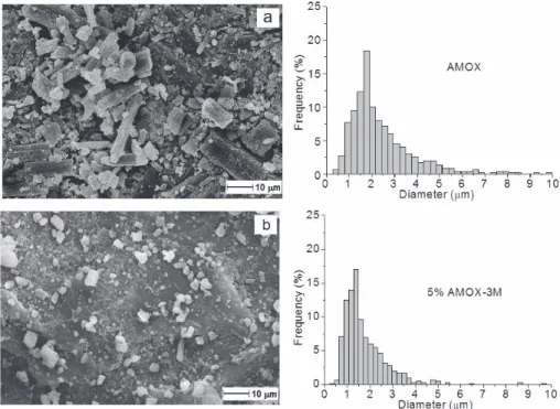
Figure IV.1 SEM micrographs and crystal dimension of amoxicillin pristine (a) and after milling with PCL (b)... 28
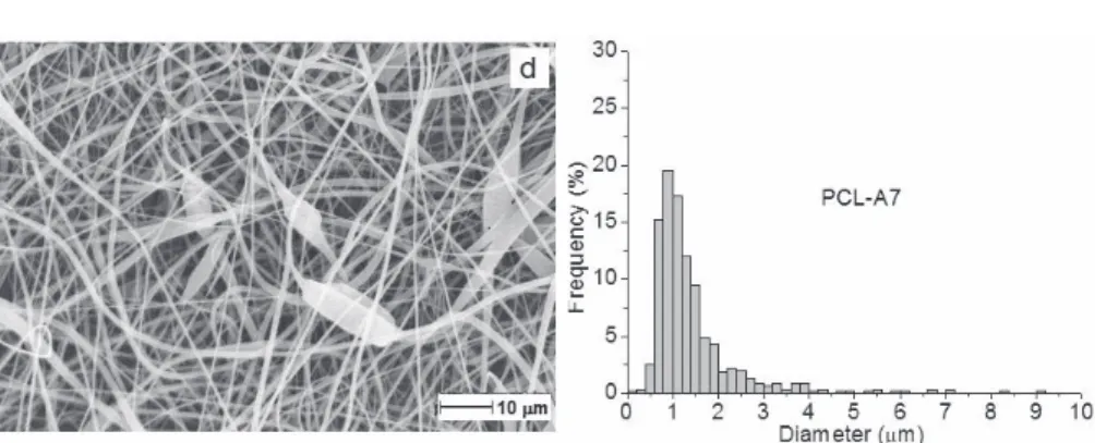
Figure IV.2 SEM micrographs and diameter distribution of PCL (a), PCL-A3 (b), PCL-A5 (c), PCL-A7 (d)... 30
Figure IV.3 SEM micrographs and diameter distribution of PCL-A5M3 (a) and PCL-A5M6 (d)... 31
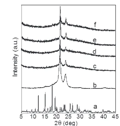
Figure IV.4 XRD diffractograms of pure AMOX (a), and after milling 3 min with PCL (b), PCL (c), PCL-A3 (d), PCL-A5 (e), and CL-A7 (f)... 32
Figure IV.5 Differential Scanning Calorimetry (DSC) curves of pure AMOX (a), PCL (b), PCL-A3 (c), PCL-A5 (d), and PCL- A7(e)... 34
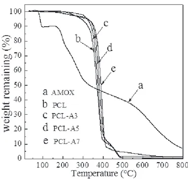
Figure IV.6 Thermogravimetric curves of pure AMOX (a), PCL(b), PCL-A3(c), PCL-A5(d), and PCL- A7(e)... 35
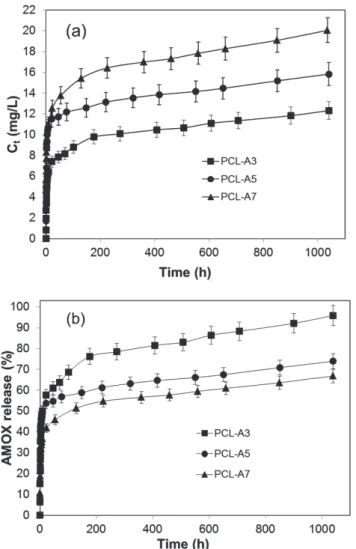
Figure IV.7 In vitro release profiles of AMOX from PCL-A3, PCL-A5 and PCL-A7, absolute concentration (Ct, mg/L) (a) and as % drug release (b) ... 37
Figure IV.8 Behavior of the first stage (- - -, extrapolate values)... 38
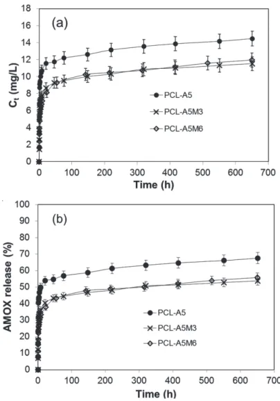
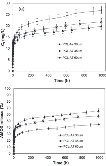
Figure IV.9 In vitro release profiles of Amoxicillin from PCL-A5, PCL-A5M3 and PCL-A5M6, absolute concentration (Ct, mg/L) (a) and as % of the maximun achievable concentration (b)... 39 Figure IV.10. In vitro release profiles of MOX from PCL-A7 30 m,
VI
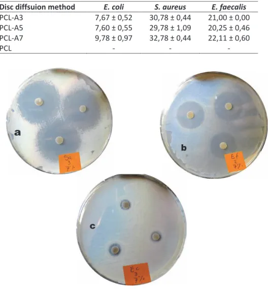
(Ct, mg/L) (a) and as % drug release (b) ... 40 Figure IV.11 Inhibitory effect of PCL-A7 against three human
patogenic bacteria by means of disc diffusion, Staphyococcus aureus (a), Enterococcus faecalis (b)
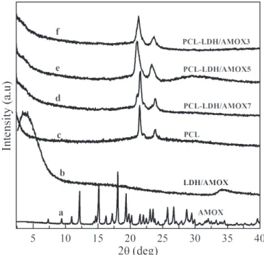
and Escherichia coli (c) ... 42 Figure V.1 AMOX intercalated into LDH………....…... 49 Figure V.2 XRD diffractograms of PCL fiber, PCL loaded with
LDH/AMOX fibers, AMOX and LDH/AMOX... 50 Figure V.3 SEM micrographs and diameter distribution of PCL (a),
PCL-LDH/AMOX3 (b), PCL-LDH/AMOX5 (c),
PCL-LDH/AMOX7(d)... 51
Figure V.4 Thermogravimetric curves of PCL fiber, PCL loaded
With LDH/AMOX fibers, AMOX and LDH/AMOX... 52 Figure V.5 Differential Scanning Calorimetry (DSC) curves of PCL
fiber, PCL loaded with LDH/AMOX fibers, AMOX and
LDH/AMOX... 53 Figure V.6 Amount of AMOX released, as absolute concentration
(Ct, mg/L) (a) and as % of the maximun achievable
concentration (b) ... 55 Figure V.7 Amount of AMOX released after 20 days... 56 Figure VI.1 SEM micrographs and diameter distribution of AMOX
(a), PLA (b), PLA-A3 (c), PLA-A5(d) and PLA-A7(e) ... 60 Figure VI.2 XRD diffractograms of PLA pellets, PLA fiber, PLA
loaded with AMOX fibers and AMOX... 61 Figure VI.3. Differential Scanning Calorimetry (DSC) curves of
PLA fibers, PLA loaded with AMOX fibers and AMOX... 62 Figure VI.4. Thermogravimetric curves of PLA fibers, PLA loaded
with AMOX fibers and AMOX... 63 Figure VI.5 In vitro release profiles of AMOX from PLA-A3, PLA-A5
and PLA-A7, absolute concentration (Ct, mg/L) (a)
and as % drug release (b)... 64 Figure VII.1 SEM micrographs and diameter distribution P75 (a),
P75-A3 (b), P75-A5 (c) and P75-A7(d)... 70 Figure VII.2 SEM micrographs and diameter distribution P50 (a),
P50-A3 (b), P50-A5 (c) and P50-A7(d)... 72 Figure VII.3 SEM micrographs and diameter distribution P25 (a),
P25-A3 (b), P25-A5 (c) and P25-A7(d)... 73 Figure VII.4 XRD diffractograms of AMOX, PLA, P75, P75-A3,
P75-A5, P75-A7 and PCL... 74 Figure VII.5 XRD diffractograms of AMOX, PLA, P50, P50-A3,
P50-A5, P50-A7 and PCL... 74 Figure VII.6 XRD diffractograms of AMOX, PLA, P25, P25-A3,
P25-A5, P25-A7 and PCL... 75 Figure VII.7 Differential Scanning Calorimetry (DSC) curves of 76
VII AMOX, PLA, P75, P75-A3, P75-A5, P75-A7 and PCL...
Figure VII.8 Differential Scanning Calorimetry (DSC) curves of
AMOX, PLA, P50, P50-A3, P50-A5, P50-A7 and PCL... 77 Figure VII.9 Differential Scanning Calorimetry (DSC) curves of
AMOX, PLA, P25, P25-A3, P25-A5, P25-A7 and PCL... 77 Figure VII. 10 Thermogravimetric curves of AMOX, PLA, P75,
P75-A3, P75-A5, P75-A7 and PCL... 79 Figure VII.11 Thermogravimetric curves of AMOX, PLA, P50,
P50-A3, P50-A5, P50-A7 and PCL... 79 Figure VII.12 Thermogravimetric curves of AMOX, PLA, P25,
P25-A3, P25-A5, P25-A7 and PCL... 80 Figure VII.13 Stress-strain curves of PLA, P75, P50, P25 and PCL…. 81 Figure VII.14 In vitro release profiles of AMOX from P75-A3,
P75-A5 and P75-A7, absolute concentration
(Ct, mg/L) (a) and as % drug release (b)... 82 Figure VII.15 In vitro release profiles of AMOX from P50-A3,
P50-A5 and P50-A7, absolute concentration
(Ct, mg/L) (a) and as % drug release (b) ... 83 Figure VII.16 In vitro release profiles of AMOX from P25-A3,
P25-A5 and P25-A7, absolute concentration
(Ct, mg/L) (a) and as % drug release (b) ... 84 Figure VII.17 Amount of AMOX released in 500 hours from:
IX
Table Content
Table II.1 Interpretation of diffusional release mechanisms from
polymeric films... 15 Table IV.1 Processing parameters and mechanical properties of
fibers fabricated by electrospinning (voltage: 30 kV,
distance: 30cm, flow rate: 4 mL/h) ... 33
Table IV.2 Thermal parameters of pure AMOX, PCL and filled PCL… 35 Table IV.3 Initial burst effect and kinetic parameters of AMOX
Release from PCL... 41
Table IV.4 Inhibition zone in mm ± SD of AMOX at different
concentrations in PCL... 42
Table V.1 LDH/AMOX content and thermal parameters... 53 Table VI.1 Composition (PLA/AMOX), processing parameters and
average diameter... 59
Table VI.2 Thermal parameters of fibers fabricated by electrospinning
(AMOX: Tm = 131 °C)... 62 Table VI.3 Initial burst, kinetic parameters and release amount of
AMOX in 500 h for PLA electrospun membranes... 65
Table VII.1 Composition (PLA/PCL/AMOX), processing parameters
and average diameter values of fibers fabricated by
electrospinning (flow rate: 4 mL/h. SD: standard deviation, diameter values are means of 500 determinations)... 69
Table VII.2. Thermal parameters of fibers fabricated by
electrospinning (AMOX: Tm = 131 °C, Midpoint
temperature = 306 °C)... 78 Table VII.3. Mechanical properties of PLA, P75, P50, P25 and PCL…. 80 Table VII.4 Initial burst, kinetic parameters and release amount of
XI
Abstract
The technical parameters for electrospinning solutions of biodegradable polymers poly(-caprolactone), poly(lactic acid) and their composites with active molecules were defined and set up. A trial-and-error approach has been employed by varying solution properties and processing parameters to obtain uniform defect-free fibers. Amoxicillin drug was intercalated in layered double hydroxide nanoparticles by coprecipitation and then the modified nanohybrid was successfully encapsulated at different concentrations into poly(-caprolactone) matrix by the electrospinning technique. Non-woven fibrous mats were fabricated and characterized in terms of morphology, in vitro release and antibacterial properties.
Blends of poly(lactic acid) and poly(ε-caprolactone), loaded with different amounts of amoxicillin were electrospun to investigate the release behaviour and obtain a controlled and tuneable release. Morphology and thermal behaviour were found dependent on the component ratio as well as on the incorporated drug amount.
XIII
Introduction
Electrospinning is a versatile method to process solutions or melts, mainly of polymers, into continuous fibers with diameters ranging from a few micrometers to a few nanometers. This technique is applicable to virtually every soluble or fusible polymer. The polymers can be chemically modified and can also be tailored with additives ranging from simple carbon-black particles to complex species such as enzymes, viruses, and bacteria. Electrospinning appears to be straightforward, but is a rather intricate process that depends on a multitude of molecular, process, and technical parameters. The method provides access to entirely new materials, which may have complex chemical structures. Electrospinning is not only a focus of intense academic investigation; the technique is already being applied in many technological area. The Electrospinning is currently the only technique that allows the fabrication of continuous fibers with diameters down to a few nanometers. The method can be applied to synthetic and natural polymers, polymer alloys, and polymers loaded with chromophores, nanoparticles, or active agents, as well as to metals and ceramics. Fibers with complex architectures, such as core–shell fibers or hollow fibers, can be produced by special electrospinning methods. It is also possible to produce structures ranging from single fibers to ordered arrangements of fibers. Electrospinning is not only employed in university laboratories, but is also increasingly being applied in industry. The scope of applications, in fields as diverse as optoelectronics, sensor technology, catalysis, filtration, and medicine, is very broad.
Electrospun nanofibers are broadly applied in biomedical applications, as tissue engineering scaffolds, in wound healing, drug delivery, filtration, as affinity membrane, in immobilization of enzymes, small diameter vascular graft implants, healthcare, biotechnology, environmental engineering, defense and security, and energy storage and generation and in various researches that are on-going (Ramakrishna et al., 2006). Since the early 1980's, electrospun polymer nanofibers have already been proposed for vascular and breast prostheses applications(Bhardwaj and Kundu, 2010). A number of US patents have been issued on fabrication methods and
XIV
techniques for these prostheses such as, covering vascular prostheses, and for breast prosthesis has been disclosed in a US patent. Reviewing the number of patents, we can see that approximately two-thirds of all electrospinning applications are in the medical field. Of the remaining patents, one-half deals with filtration applications, and all other applications share the remaining half. Owing to application of these nanofibers in diverse fields, various research and developments are going in the fields of electrospinning (Burger et al., 2006).
In the recent literature shows the tendency to the production of nanofibers nanocomposite for biomedical applications, applications are becoming more specific, so it should work with biodegradable polymers with specific characteristics and suitable properties, likewise the drug should be chosen carefully for our future research will have repercussions.
The aim of this work is to study and optimize electrospinning process for the production of nanofibers and nanocomposites nanofibers.
The principal objective of the work is the production of micro and nanofibers of polymers loaded with active molecules.
For the production of micro-and nanofiber nanocomposite are several parameters that should be taken into account, also take into consideration the drug release profiles and the biodegradability of the polymer. This work will focus on the following point: study of different polymer solution parameters (Concentration, viscosity, conductivity, surface tension, dielectric constant); study of different processing conditions (voltage, federate, temperature, diameter of needle, distance between tip and collector); study of ambient parameters (humidity, type of atmosphere, pressure); product characterizations (solid state characterization, drug loading, release profiles); mathematical modelling of release kinetics of a selected systems of interest.
1
Chapter I
Electrospinning
I.1 Introduction
In the late 1500s William Gilbert set out to describe the behaviour of magnetic and electrostatic phenomena. His work is an early example of what would become the modern scientific method (Gilbert, 1600). He received funding from Queen Elizabeth I, whereupon he moved to London, caught bubonic plague, and passed away. He had, however, already distinguished between the magnetic forces arising from a lodestone (natural magnet) and the electrostatic forces arising from rubbed amber. One of his more obscure observations was that when a suitably charged piece of amber was brought near a droplet of water it would form a cone shape and small droplets would be ejected from the tip of the cone the first recorded observation of electrospraying.
The first description of a process recognisable as electrospinning was in 1902 when J. F. Cooley filed a United States patent entitled “Apparatus for electrically dispersing fibres” (Cooley, 1902). In his patent he describes a method of using high voltage power supplies to generate yarn. Even at this early stage it was recognised that to form fibres rather than droplets the (i) fluid must be sufficiently viscous, (ii) solvent volatile enough to evaporate to allow regeneration of the solid polymer, and (iii) electric field strength within a certain range.
The next significant academic development was achieved by John Zeleny, who published work on the behaviour of fluid droplets at the end of metal capillaries in 1914 (Zeleny, 1914). His work began the efforts to mathematically model the behaviour of fluids under electrostatic forces. Between 1964 and 1969, Sir Geoffrey Ingram Taylor produced the theoretical underpinning of electrospinning (Taylor, 1964, 1966, 1969).
Electrospinning
2
Taylor’s work on electrostatics was performed during his retirement after a broad career including modelling of turbulent mixing of air at the Arctic, significant contributions to the fields of fluid mechanics and solid mechanics via work on the Manhattan Project and development of supersonic aircraft. Taylor’s work contributed to electrospinning by mathematically modelling the shape of the cone formed by the fluid droplet under the effect of an electric field; this characteristic droplet shape is now known as the Taylor cone. He further worked with J.R. Melcher to develop the ‘leaky dielectric model’ for conducting fluids (Melcher and Taylor, 1969).
In parallel to the academic work of Zeleny and Taylor came a sequence of patents, starting with the design by Cooley who separated the charging device from the spinning head (Cooley, 1902). In the same year, Morton patented a simpler low-throughput machine (Morton, 1902). Melt spinning and air-blast assist were proposed by Norton (Norton, 1936) then a sequence of constant pressure feed high-throughput machines by Anton Formhals was filed between 1934 and 1944 to produce continuous fine fibres for use on standard textile machinery (Formhals, 1934, 1938, 1939, 1940, 1943, 1944). Gladding also proposed the use of the process to produce staple (discontinuous fibres) (Gladding, 1939).
Electrospinning was re-discovered in 1995 in the form of a potential source of nano-structured material by Doshi and Reneker who, whilst investigating electrospraying, observed that fibres could easily be formed with diameters on the nanometre scale(Doshi and Reneker, 1995). Huang and co-workers noted that between 1995 and 2000 fewer than 10 journal papers were published annually, but from 2000 onwards the number of papers per year grew, reaching over 50 by 2002 and reflecting the growing interest in electrospinning by, at least, the academic community (Huang et al., 2003).
Since 1995 there have been further theoretical developments of the driving mechanisms of the electrospinning process. Reznik and co-workers describe extensive work on the shape of the Taylor cone and the subsequent ejection of a fluid jet (Reznik et al., 2004). The work by Hohman and co-workers investigates the relative growth rates of the numerous proposed instabilities in an electrically forced jet once in flight. Also important has been the work by Yarin and co-workers that endeavours to describe the most important instability to the electrospinning process, the bending (whipping) instability(Yarin et al., 2001). The term ‘electrospinning’ was first coined in 1995 by Doshi and Reneker (Doshi and Reneker, 1995).
For improvement in the applicability of these fibers, various new innovations electrospinning are being used. These innovations include coaxial electrospinning, mixing and multiple electrospinning, core shelled electrospinning, blow assisted electrospinning and others.
Chapter I
3 Coaxial electrospinning includes fabrication of nanofibers from two polymers which utilizes coaxial capillary spinneret and as a result a core of one polymer and shell of the other are formed (Sun et al., 2003). With this technology, some polymers which are difficult to process are coelectrospun and form a core inside the shell of other polymer. This method gains attention as it provides novel properties and functionalities of nanoscale devices through the combination of polymeric materials in the axial and radial direction. The electrospun nanofibers are also used as drug delivery vehicles, but due to large surface area and high porosity, a significant burst release is observed. Coaxial method is commonly used for controlling the burst release of drugs, as the shell of the polymer acts as diffusion barrier for drugs. Other new innovations will also offer various advantages. Blowing-assisted electrospinning helps in spinning of high molecular weight polymers which was otherwise difficult to spin by solution electrospinning. Recently, there has been wide interest in using the nanofibrous membranes as tissue engineering scaffolds. A nanoscale fibrous scaffold more closely mimics the extracellular matrix than macroscale scaffolds and provides a three dimensional (3D) environment. With nanofibrous scaffolds, cell adhesion, proliferation and differentiation of several types of cells have been observed including bone marrow stem cells too. As a tissue engineering scaffolds, nanofibers of various polymers can be used for osteogenesis, wound healing, skin regeneration. Therefore, an electrospun nanofibrous scaffold holds great potential to be used for tissue engineering applications in future. A recent research has demonstrated the use of nanofibers in making nanowires as the incorporation of carbon nanotubes within the fibrous structure provides anisotropic properties such as electrical and thermal conductivity (Hunley and Long, 2008). With the advent of copolymerization and polymer mixtures, attainment of the desired physical and biological properties of nanofibrous mesh has become possible now. There is on-going research for the improvement of nanofiber properties and the scale up of this process. In future electrospun nanofibers will prove to be a promising candidate for a wider range of applications (Bhardwaj and Kundu, 2010).
I.2 Electrospinning Process
The process of electrospinning, namely utilizing electrostatic forces to generate polymer fibers, traces its roots back to the process of electrospraying, in which solid polymer droplets are formed rather than fibers. In fact, a number of processing parameters must be optimized in order to generate fibers as opposed to droplets, and a typical electrospinning apparatus can be used to form fibers, droplets, or a beaded structure depending on the various processing parameters, such as distance between source and collector. In recent work, a greater understanding of processing
Electrospinning
4
parameters has led to the formation of fibers with diameters in the range of 100-500 nm, typically referred to as nanofibers. The development of nanofibers has led to resurgence in interest regarding the electrospinning process due to potential applications in filtration, protective clothing, and biological applications such as tissue engineering scaffolds, and drug delivery devices (Sill and von Recum, 2008).
A typical electrospinning setup consists of a capillary through which the liquid to be electrospun is forced; a high voltage source with positive or negative polarity, which injects charge into the liquid; and a grounded collector. A syringe pump, gravitational forces, or pressurized gas are typically used to force the liquid through a small-diameter capillary forming a pendant drop at the tip. An electrode from the high voltage source is then immersed in the liquid or can be directly attached to the capillary if a metal needle is used. The voltage source is then turned on and charge is injected into the polymer solution. Increasing the electric field strength causes the repulsive interactions between like charges in the liquid and the attractive forces between the oppositely charged liquid and collector to begin to exert tensile forces on the liquid, elongating the pendant drop at the tip of the capillary. As the electric field strength is increased further a point will be reached at which the electrostatic forces balance out the surface tension of the liquid leading to the development of the Taylor cone. If the applied voltage is increased beyond this point a fiber jet will be ejected from the apex of the cone and be accelerated toward the grounded collector. While the fiber jet is accelerated through the atmosphere toward the collector it undergoes a chaotic bending instability, thereby increasing the transit time and the path length to the collector and aiding in the fiber thinning and solvent evaporation processes. Yarin et al. have suggested that this bending instability is due to repulsive interactions between like charges found in the polymer jet (Yarin et al., 2001). Doshi and Reneker had hypothesized that charge density increases as the fiber jet thins, dramatically increasing radial charge repulsion which causes the fiber jet to split into a number of smaller fibers when a critical charge density is met (Doshi and Reneker, 1995). However, in more recent studies high-speed photography has been used to image the unstable zone of the fiber jet, revealing that a whipping instability causes the single fiber to bend and turn rapidly giving the impression that the fiber is splitting (Shin et al., 2001a).
The solid polymer fibers are then deposited onto a grounded collector. Depending on the application a number of collector configurations can be used, including a stationary plate, rotating mandrel, solvent (e.g. water), etc. Typically the use of a stationary collector will result in the formation of a randomly oriented fiber mat. A rotating collector can be used to generate mats with aligned fibers, with the rotation speed playing an important role in determining the degree of anisotropy. Additionally, Liu and Hsieh found that
Chapter I
5 both the conductivity and the porosity of the collector play an important role in determining the packing density of the collected fibers (Liu and Hsieh, 2002).
The parameters affecting electrospinning and the fibers may be broadly classified into processing parameters, solution parameters and ambient parameters. With the understanding of these parameters, it is possible to come out with setups to yield fibrous structures of various forms and arrangements. It is also possible to create nanofiber with different morphology by varying the parameters.
I.2.1 Processing parameters
Despite electrospinning’s relative ease of use, there are a number of processing parameters that can greatly affect fibers formation and structure. Grouped in order of relative impact to the electrospinning process, these parameters are applied voltage, polymer flow rate, capillary-collector distance, collector geometry, collector material, diameter of pipette orifice/needle and temperature. Furthermore, all parameters can influence the formation of bead defects.
I.2.1.1 Applied voltage
The strength of the applied electric field controls formation of fibers from several microns in diameter to tens of nanometers. Suboptimal field strength could lead to bead defects in the spun fibers or even failure in jet formation. Deitzel et al. examined a polyethylene oxide (PEO)/water system and found that increases in applied voltage altered the shape of the surface at which the Taylor cone and fiber jet were formed (Deitzel et al., 2001). At lower applied voltages the Taylor cone formed at the tip of the pendent drop; however, as the applied voltage was increased the volume of the drop decreased until the Taylor cone was formed at the tip of the capillary, which was associated with an increase in bead defects seen among the electrospun fibers.
I.2.1.2 Flow rate
The flow rate will determine the amount of solution available for electrospinning. For a given voltage, there is a corresponding flow rate if a stable Taylor cone is to be maintained. When the flow rate is increased, there is a corresponding increase in the fiber diameter or beads size, this is apparent as there is a greater volume of solution that is drawn away from the needle tip (Rutledge et al., 2000; Zong et al., 2002).
Electrospinning
6
I.2.1.3 Capillary-collector distance
While playing a much smaller role, the distance between capillary tip and collector can also influence fiber size by 1-2 orders of magnitude. Additionally, this distance can dictate whether the end result is electrospinning or electrospraying. Doshi and Reneker found that the fiber diameter decreased with increasing distances from the Taylor cone (Doshi and Reneker, 1995).
I.2.2 Solution parameters
In addition to the processing parameters a number of solution parameters play an important role in fiber formation and structure. In relative order of their impact on the electrospinning process these include polymer concentration, solvent volatility, solvent conductivity, surface tension, molecular weight and solution viscosity and dielectric effect of solvent (dielectric constant ).
I.2.2.1 Polymer concentration
At concentrations allowing adequate chain entanglement, continuous uniform nanofibers can be electrospun from polymer solutions in a strong enough electric field (Deitzel et al., 2001; Pornsopone et al., 2005). The concentration of polymer in solution often determines if it wills electrospin at all and generally has a dominant effect on the fiber diameter, as well as fiber morphology (Demir et al., 2002).
I.2.2.2 Solvent volatility
Invariably, it is the evaporation of solvent from the jet that yields a solid polymer nanofiber at the collector plate. Ideally, all traces of solvent must be removed by the time the nanofiber hits the collector. If not, the wet fibers may fuse together to form a melded or reticular mat. Sometimes a flat ribbon-like nanofibers derived from the fluid–filled, incompletely dry nanofiber due to slow subsequent evaporation of solvent and collapse of the tube, are obtained (Koombhongse et al., 2001).
I.2.2.3 Solution conductivity
Electrospinning involves stretching of the solution caused by repulsion of the charges at its surface. Thus if the conductivity of the solution is increased, more charges can be carried by the electrospinning jet. The conductivity of the solution can be increased by the addition of ions.
Chapter I
7 Moreover, most drugs and proteins form ions when dissolved in water. As previously mentioned, beads formation will occur if the solution is not fully stretched. Therefore, when a small amount of salt or polyelectrolyte is added to the solution, the increased charges carried by the solution will increase the stretching of the solution. As a result, smooth fibers are formed which may otherwise yield beaded fibers. The increased in the stretching of the solution also will tend to yield fibers of smaller diameter (Zong et al., 2002).
I.2.3 Ambient Parameters
The effect of the electrospinning jet surrounding is one area which is still poorly investigated. Any interaction between the surrounding and the polymer solution may have an effect on the electrospun fiber morphology. Ambient parameters include humidity, type of atmosphere and pressure. High humidity for example was found to cause the formation of pores on the surface of the fibers. Since electrospinning is influenced by external electric field, any changes in the electrospinning environment will also affect the electrospinning process.
Electrospinning
9
Chapter II
Composite nanofibers
II.1 Nanofibers
Nanofibers are defined as fibers with diameters on the order of 1000 nanometers. They can be produced by a variety of techniques such as phase separation, self-assembly, drawing, melt fibrillation, template synthesis, interfacial polymerization, solution spinning and electrospinning. Nanofibers reduce the handling problems mostly associated with the nanoparticles. Nanoparticles can agglomerate and form clusters, whereas nanofibers form a mesh that stays intact even after regeneration. Nanofibers are used in medical applications, which include drug and gene delivery, artificial blood vessels, artificial organs and medical facemasks (Chang, 2009).
The nanofibers produced by electrospinning technique are commonly called electrospun fibers or electrospun nanofibers. They can be used in several applications: nonwoven fabrics, reinforced fibres, support for enzymes, drug delivery systems, fuel cells, conducting polymers and composites, photonics, sensorics, medicine, pharmacy, wound dressings, filtration, tissue engineering, catalyst supports, fibre mats serving as reinforcing component in composite systems, and fibre templates for the preparation of functional nanotubes, to name just a few.
The accumulation of non-woven or aligned fibers produces the so called fibrous mats (Charernsriwilaiwat et al., 2010), fibrous fabrics (Chegoonian et al., 2012) or fibrous membranes (Chen et al., 2011). For instance, a pore structured electrospun nanofibrous membrane used as a wound dressing can promote the exudation of fluid from the wound, so as to prevent either build-up under the covering or wound desiccation. The electrospun nanofibrous membrane shows controlled liquid evaporation, excellent oxygen permeability and promoted fluid drainage capacity, while still inhibiting exogenous microorganism invasion because its ultrafine pores. Fibre mats
Composite nanofibers
10
serving as reinforcing component in composite systems, and fibre templates for the preparation of functional nanotubes (He et al., 2008).
Nanofibers will also eventually find important applications in making nanocomposites. This is because nanofibers can have even better mechanical properties than micro fibers of the same materials, and hence the superior structural properties of nanocomposites can be anticipated. Moreover, nanofiber reinforced composites may possess some additional merits which cannot be shared by traditional (microfiber) composites (Huang et al., 2003).
II.2 Nanocomposite
A nanocomposite is a multiphase solid material where one of the
phases has one, two or three dimensions of less than 100 nm, or
structures having nano-scale repeat distances between the different
phases that make up the material (Ajayan et al., 2006).
The synthesis of polymer nanocomposites is an integral aspect of
polymer nanotechnology. By inserting the nanometric inorganic
compounds, the properties of polymers improve and hence this has a
lot of applications depending upon the inorganic material present in
the polymers. Polymer nanocomposites are materials in which
nanoscopic inorganic particles, typically 10-100 Å in at least one
dimension, are dispersed in an organic polymer matrix in order to
dramatically improve the performance properties of the polymer
(Lagashetty and Venkataraman, 2005). Systems in which the
inorganic particles are the individual layers of a lamellar compound -
most typically a smectite clay or nanocomposites of a polymer (such
as nylon) embedded among layers of silicates – exhibit dramatically
altered physical properties relative to the pristine polymer. Polymer
nanocomposites represent a new alternative to conventionally filled
polymers. Because of their nanometer sizes, filler dispersion
nanocomposites exhibit markedly improved properties when
compared to the pure polymers or their traditional composites. These
include increased modulus and strength, outstanding barrier
properties, improved solvent and heat resistance and decreased
flammability.
There are three types of nanocomposites, depending on how many
dimensions of the dispersed particles are in the nanometer range can
be distinguished (Alexandre and Dubois, 2000). Particles with three
dimensions in the order of nanometers are typically isodimensional,
such as spherical silica nanoparticles obtained by in situ sol-gel
Chapter II
11
methods (Mark, 1996; Reynaud et al., 1999) or by polymerization
promoted directly from their surface (Reynaud et al., 1999; Von
Werne and Patten, 1999). They also include semiconductor
nanoclusters (Herron and Thorn, 1998) and others (Reynaud et al.,
1999). Nanotubes or whiskers (with dimensions in the nanometer
scale and the third forming a larger elongated structure), for example,
carbon nanotubes or cellulose whiskers (Chazeau et al., 1999; Favier
et al., 1997), are extensively studied as reinforcing phases yielding
materials with
exceptional properties. The third type
of
nanocomposites is characterized by only one dimension in the
nanometer range. In this case the material is present in the form of
sheets of one to a few nanometers thick and hundreds to thousands
nanometers long. This family of composites is referred to as
polymer-layered crystal nanocomposites (Mojumdar and Raki, 2005).
Depending on the nature of the components used (layered structure,
organic ions/polymer matrix) and the method of preparation, three
main types of composites composites may be obtained when a layered
structure is associated with a polymer (Alexandre and Dubois, 2000).
If the polymer is unable to intercalate between the layered sheets, a
phase-separated composite is obtained, whose properties stay in the
same range as traditional microcomposites. Beyond this classical
family of composites, two types of nanocomposites can be
distinguished. An ‘intercalated’ structure in which a single (and
sometimes more than one) extended polymer chain is intercalated
between the inorganic layers resulting in a well-ordered multilayer
morphology built up with alternating polymeric and inorganic layers.
When the layers are completely and uniformly dispersed in a
continuous polymer matrix, an ‘exfoliated or delaminated’ structure is
obtained.
II.3 Composite Nanofibers
It is a general practice in polymer technology to compound inorganic (and sometimes even organic) fillers into a polymer matrix to either reduce the cost of a formulation or to improve its mechanical properties. Fillers used in the latter case are reinforcing fillers and must be of small enough average particle size and of adequate surface compatibility with the matrix to effectively play this crucial role. Ideally, the particle size should be smaller than the interchain distances in the polymer matrix to avoid the introduction of points of local stress into the material. For instance, in elastomers only filler particles smaller than about a micrometer result in significant levels of
Composite nanofibers
12
reinforcement, with better composite properties obtained at even smaller particle sizes. Larger particles of filler (>10 microns) typically reduce the mechanical properties of composites. Qualitatively, the mechanism of reinforcement in composites is via the transfer of stresses propagating through the polymer to the higher-modulus filler particles. High specific surface area and larger aspect ratio of the filler as well as good compatibility between the filler and polymer will determine the efficiency of load transfer and invariably the degree of reinforcement. Reinforcing fillers are often surface treated to alter their chemistry (e.g., silica might be treated with, 1% by weight of aminosilane) to allow better wetting or closer interaction of filler with the polymer. Carbon nanotubes and carbon fibers have been extensively researched to improve their function as potential reinforcing fillers in polymer composites (Andrady, 2008).
Composite materials owe their exceptional mechanical and other useful properties to the existence of an extensive interface fraction localized at the phase boundary between filler and bulk resin. The larger the fractional interface, the more pronounced will be its influence on the properties of the composite. With a compatible filler material the interface is more complex than a simple two-dimensional contact region between the particle and polymer. The interface “layer” formed around the particle has a finite thickness, and within it the material properties are very different from those in the bulk (Pukánszky, 2005).
II.3.1 Polymer–clay composites
A majority of studies on composite nanofibers reinforced with clays has been on montmorillonite (MMT), a clay with plate-like particles having a chemical composition of hydrated sodium calcium aluminum magnesium silicate hydroxide (Na,Ca)0.33(Al,Mg)2(Si4O10)(OH)2.nH2O (value of n varies with the degree of hydration). The platelets of the clay have a high modulus (170GPa), a high aspect ratio (1000nm x75–100nm), a surface area of 750 m2 per g, are hydrophilic, and occur in aggregated form or as tactoids. These have to be dispersed into individual platelets to exploit their high surface area in reinforcing polymers (Hong et al., 2005).
II.3.2 Drug-loaded fibers
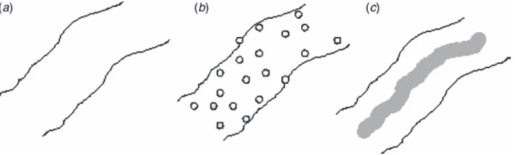
The kinetics of release of the drug is controlled by the semicrystalline nature of the polymer as well as by the morphology of the polymer/drug composite. Three basic morphological models (Figure II.1) for drug-loaded polymers (or polymer particles), first proposed by Kissel et al. (Kissel et al., 1993), apply to drug-loaded nanofibers as well (Verreck et al., 2003):
Chapter II
13 a. Drug dissolved in the polymer matrix at the molecular level.
b. Drug distributed in the polymer matrix as crystalline or amorphous particles.
c. Drug enclosed in the polymer matrix yielding a core of the drug encapsulated by a polymer layer (similar to a reservoir device).
Figure II.1 Illustration of the three morphological models of drug-loaded
polymer nanofibers.
II.3.2.1 Drug delivery
The simplest configuration of a controlled release device is where a drug is either dissolved in high concentration or suspended as particles in a monolithic polymer such as a cylindrical polymer fiber (Andrady, 2008). The release of the drug from it may occur via:
1. Diffusive transfer through the polymer matrix to the surrounding tissue.
2. Release of the dissolved or suspended drug due to slow biodegradation or erosion of the surface layers of the fiber.
3. Slow release of covalently bonded drug via hydrolytic cleavage of the linkages.
4. Rapid delivery of the drug due to dissolution of the fiber.
In vitro dissolution has been recognized as an important element in drug development. Under certain conditions it can be used as a surrogate for the assessment of Bioequivalence. Several theories / kinetics models describe drug dissolution from immediate and modified reléase dosage forms. There are several models to represent the drug dissolution profiles where ft (fraction of drug dissolved in time t) is a function of t (time) related to the amount of drug dissolved from the pharmaceutical dosage system. The quantitative interpretation of the values obtained in the dissolution assay is facilitated by the usage of a generic equation that mathematically translates the dissolution curve in function of some parameters related with the pharmaceutical dosage forms. In some cases, that equation can be deduced
Composite nanofibers
14
by a theoretical analysis of the process, as for example in zero order kinetics. In most cases, with tablets, capsules, coated forms or prolonged release forms that theoretical fundament does not exist and sometimes a more adequate empirical equations is used. The kind of drug, its polymorphic form, cristallinity, particle size, solubility and amount in the pharmaceutical dosage form can influence the release kinetic (Ei-Arini and Leuenberger, 1995; Salomon and Doelker, 1980). A water-soluble drug incorporated in a matrix is mainly released by diffusion, while for a low water-soluble drug the self-erosion of the matrix will be the principal release mechanism. To accomplish these studies the cumulative profiles of the dissolved drug are more commonly used in opposition to their differential profiles. To compare dissolution profiles between two drug products model dependent (curve fitting), statistic analysis and model independent methods can be used (Costa and Sousa Lobo, 2001).
The quantitative interpretation of the values obtained in dissolution assays is easier using mathematical equations which describe the release profile in function of some parameters related with the pharmaceutical dosage forms. Some of the most relevant and more commonly used mathematical models describing the dissolution curves are:
Zero order: Qt = Q0 + K0t (II.1) First order: ln Qt = ln Q0 + K1t (II.2) Second order: Qt /Q∞ (Q∞ – Qt )K2 t (II.3) Hixson–Crowell Q01/3 – Qt1/3 = Kst (II.4) Weibull log[-ln(1 – ( Qt /Q∞ ))]= b x log t – log a (II.5) Higuchi Qt = KH√ (II.6) Baker–Lonsdale (3/2)[1 – (–1(Qt /Q∞))2/3 ] – (Qt /Q∞) = Kt (II.7) Korsmeyer–Peppas Qt /Q∞ = Kk tn (II.8) Quadratic Qt = 100(K1 t 2 + K2 t) (II.9) Logistic Qt = A/ [1 + e–K(t – y)] (II.10) Gompertz Qt = A e –e – K(t – y) (II.11) Hopfenberg Qt /Q∞ = 1 – [1 – k0 t/C0a0 ] (II.12) where Qt is the amount of drug dissolved in time t, Q0 is initial amount of drug in the solution (most times, Q0 = 0), K0 is the zero order release constant, K1 is the first order release constant, Q∞ is the amount of drug released at
an infinite time, K2 is the second order release constant, Ks is a constant incorporating the surface–volume relation, the scale parameter, a, defines the time scale of the process. The shape parameter, b, characterizes the curve as either exponential (b = 1) (Case 1), sigmoid, S-shaped, with upward curvature followed by a turning point (b.1) (Case 2), or parabolic, with a
Chapter II
15 higher initial slope and after that consistent with the exponential (b > 1) (Case 3), where KH is the Higuchi dissolution constant, the release constant, k, corresponds to the slope, Kk is the Korsmeyer–Peppas release constant, n is the release exponent, indicative of the drug release mechanism,Peppas (Peppas, 1985) used this n value in order to characterize different release mechanisms, concluding for values for a slab, of n = 0.5 for Fick diffusion and higher values of n, between 0.5 and 1.0, or n = 1.0, for mass transfer following a non-Fickian model (Table II.1). In the case of a cylinder, k0 is the erosion rate constant, C0 is the initial concentration of drug in the matrix and a0 is the initial radius for a sphere or cylinder or the half-thickness for a slab (Costa and Sousa Lobo, 2001).
The drug transport inside pharmaceutical systems and its release sometimes involves multiple steps provoked by different physical or chemical phenomena, making it difficult, or even impossible, to get a mathematical model describing it in the correct way. These models better describe the drug release from pharmaceutical systems when it results from a simple phenomenon or when that phenomenon, by the fact of being the rate-limiting step, conditions all the other processes.
Table II.1 Interpretation of diffusional release mechanisms from polymeric
films Release exponent (n) Drug transport mechanism Rate as a function of time 0.5 Fickian diffusion t - 0.5 0.5 < n < 1.0 Anomalous transport tn - 1
1.0 Case-II transport Zero order release
Higher than 1.0 Super Case-II transport tn - 1
The release models with major appliance and best describing drug release phenomena are, in general, the Higuchi model, zero order model, Weibull model and Korsmeyer–Peppas model. The Higuchi and zero order models represent two limit cases in the transport and drug release phenomena, and the Korsmeyer–Peppas model can be a decision parameter between these two models. While the Higuchi model has a large application in polymeric matrix systems, the zero order model becomes ideal to describe coated dosage forms or membrane controlled dosage forms.
Composite nanofibers
17
Chapter III
Methods of investigation and
Materials
III.1 Methods
III.1.1 Differential Scanning Calorimetry (DSC)
DSC measurements were carried out using a Mettler DSC 822/400
thermal analyzer instrument having sub-ambient capability. About 2-3
mg sample was placed in an aluminium pan and heated at a rate of 10
°C/min from 0 to 250 °C in a nitrogen atmosphere.
III.1.2 Thermogravimetric Analysis (TGA)
Thermoanalytical characterizations were performed by a Mettler
TC-10 thermobalance operating at 5 °C/min heating rate, under air
flow, from 25 to 800 °C. Degradation temperature (T
d) is reported as
the midpoint of the degradation step.
III.1.3 X-ray Diffraction (XRD)
XRD data were collected using an automatic Bruker diffractometer (equipped with a continuous scan attachment and a proportional counter), with the nickel filtered Cu K radiation ( = 1.54050 Å) and operating at 40 kV and 40 mA. The diffraction scans were recorded at 2 = 2-40°, step scan 0.03° of 2θ and 3s of counting time.
Methods of investigation and Materials
18
III.1.4 Scanning Electron Microscopy (SEM)
The morphology and the diameter of the electrospun nanofibers were analysed by a scanning electron microscope (SEM Mod. LEO 420, Assing, Italy). All samples were sputter coated with gold (Agar Automatic Sputter Coater Mod.B7341, Stansted, UK) at 40 mA for 180 s prior the analysis. The fibers diameter distribution was determined by Sigma SacnPro 5. About 500 fibers were considered, taking their dimensions respect to the reference bar of SEM image.
III.1.5 Ultraviolet Spectroscopy (UV-VIS)
The in vitro study of amoxicillin release was performed by measuring the absorbance at 228 nm using an ultraviolet spectrophotometer (model UV-2401, SHIMADZU). The tests were performed using rectangular specimen of 25 cm2 placed into 25 mL of physiological saline solution, stirred at room temperature and 100 rpm in an orbital shaker (VDRL MOD. 711+, Asal S.r.l.). The release medium was withdrawn at fixed time intervals and replenished with fresh medium.
III.1.6 High Energy Ball Milling (HEBM)
Milling was carried out using a Retsch PM100 planetary milling at 600 rpm, PCL with amoxicillin was prepared by mixing 3.8 g of PCL with 0.2 g of AMOX in a 50 mL Retsch stainless steel vessel with five 10 mm diameter stainless. Milling was performed in 1.5 min intervals, followed by a 10 s pause.
III.1.7 Mechanical properties
The Young’s modulus, tensile strength and the strain at break of the fibers were measured using a dynamometric apparatus INSTRON (model 4301). The instrument is interfaced to a PC with a software "Series IX" for data acquisition. The measurements were carried out at room temperature at a deformation rate of 10 mm/min. The length, thickness and width were measured for each sample (approximately 20 × 10 × 0.03 mm).
III.1.8 Antibacterial activities in vitro
The inhibitory activity of the electrospun nanofibers charged with different concentrations of AMOX was evaluated by the disc diffusion method according to the specifications of the document M2-A9 from the
Chapter III
19 Clinical and Laboratory Standards Institute (Clinical and Laboratory Standards Institute, 2006b). A criogenic (-80 °C) reserve of each strain was used to make the overnight broth culture. An aliquot of the criogenic reserve of S. aureus and E. coli was inoculated in two 7 ml Tryptic soy broth tubes while E. faecalis was inoculated in 7 ml BHI broth. Each bacteria was adjusted to 0,5 McFarland in 0,9% sodium chloride solution previous to the inoculation in MHA plates. Three membranes in shape of disc of 6 mm diameter were placed onto MHA plates. The procedure was repeated three times per bacteria. The plates were inverted face down and incubated at 35 °C for 24 hours. AMOX work solution (1mg/mL) was used as positive control(Clinical and Laboratory Standards Institute, 2006a), three 6 mm diameter wells were made in three MHA plates, one per strain, 25 l of the AMOX work solution was injected in each well. The activity against the same three bacteria was evaluated using the agar well diffusion method as described by Boyanova et al. (Boyanova et al., 2005) and Kroiss et al. (Kroiss et al., 2010). As negative control, five 6 mm diameter discs of nanofibers without AMOX were sterily placed onto one MHA plate and incubated under the same conditions above. All data were statistical analyzed by means of Student’s t-test with 0,05.
III.2 Materials
III.2.1 Poly(
-caprolactone) (PCL)
Poly(-caprolactone) (PCL) is a semi-crystalline biodegradable polyester with a glass transition temperature of about −60°C and a low melting point of around 60°C, which could be a handicap in some applications. Therefore, PCL is generally blended (Averous et al., 2000) or modified (e.g., copolymerisation, crosslink (Tan et al., 2012)). Two main pathways to produce polycaprolactone have been described in the literature: the polycondensation of a hydroxycarboxylic acid: 6-hydroxyhexanoic acid, and the ring-opening polymerisation (ROP) of a lactone: -caprolactone (-CL) in the presence of aluminium isopropoxide (Albertsson and Varma, 2002; Chiellini and Solaro, 1996; Okada, 2002). Figure III.1 gives the chemical structure of this polyester.
Methods of investigation and Materials
20
This synthetic polymer is currently used in a number of biomedical applications due to its mechanical properties, miscibility with a large range of other polymers, biocompatibility (Kim et al., 2004b), biodegradability, good drug permeability and slow biodegradability (Lannutti et al., 2007). PCL is widely used in the manufacture of speciality polyurethanes. Polycaprolactones impart good water, oil, solvent and chlorine resistance to the polyurethane produced. This polymer is often used as an additive for resins to improve their processing characteristics and their end use properties (e.g., impact resistance). Being compatible with a range of other materials, PCL can be mixed with starch to lower its cost and increase biodegradability or it can be added as a polymeric plasticizer to Polyvinyl chloride (PV). But, it finds also some application based on its biodegradable character in domains such as controlled release of drugs, soft compostable packaging. Polycaprolactone is also used for splinting, modeling, and as a feedstock for prototyping systems.
PCL is considered a non-toxic and a tissue compatible material (Gunatillake and Adhikari, 2003). It is being investigated as a scaffold for tissue repair via tissue engineering, GBR membrane. It has been used as the hydrophobic block of amphiphilic synthetic block copolymers used to form the vesicle membrane of polymersomes. A variety of drugs have been encapsulated within PCL beads for controlled release and targeted drug delivery which have been peer reviewed (Surendran et al., 2012).
Tokiwa and Suzuki have discussed the hydrolysis of PCL and biodegradation by fungi. They have shown that PCL can be easily enzymatically degraded (Tokiwa and Suzuki, 1977). According to Bastioli, the biodegradability can be clearly claimed but the homoplymer hydrolysis rate is very low (Bastioli, 1998). The presence of starch can significantly increase the biodegradation rate of PCL. PCL is degraded by hydrolysis of its ester linkages in physiological conditions (such as in the human body) and has therefore received a great deal of attention for use as an implantable biomaterial. In particular it is especially interesting for the preparation of long term implantable devices, owing to its degradation which is even slower than that of polylactide (Ibrahim et al., 2009).
III.2.2 Poly(lactic acid) (PLA)
Polylactic acid or polylactide (PLA) is a thermoplastic aliphatic polyester derived from renewable resources, such as corn starch (in the United States), tapioca roots, chips or starch (mostly in Asia), or sugarcane (in the rest of the world). It can biodegrade under certain conditions, such as the presence of
Chapter III
21 oxygen and without the presence of oxygen. This is a biodegradable polymer with different biomedical applications because of its mechanical properties and biocompatibility (Kim et al., 2004b). Figure III.2 shows the chemical structure of this polymer.
Figure III.2 Chemical structure of Poly(lactic acid)
There are several industrial routes to produce poly(lactic acid). Two main monomers are used: lactic acid, and the cyclic di-ester, lactide. The most common route to poly(lactic acid) is the ring-opening polymerization (ROP) of lactide with various metal catalysts (typically tin octoate) in solution, in the melt, or as a suspension. The metal-catalyzed reaction tends to cause racemization of the poly(lactic acid), reducing its stereoregularity compared to the starting material (Södergård and Stolt, 2010). Another route to produce poly(lactic acid) is the direct condensation of lactic acid monomers.
Poly(lactic acid) can be processed by extrusion, injection molding, film and sheet casting, spinning, providing access to a wide range of materials. Being able to degrade into innocuous lactic acid, poly(lactic acid) is used as medical implants in the form of screws, pins, rods, and as a mesh. Depending on the exact type used, it breaks down within the body within 6 months to 2 years. This gradual degradation is desirable for a support structure, because it gradually transfers the load to the body (e.g. the bone) as that organ heals. PLA can also be used as a compostable packaging material, either cast, injection molded, or spun. Cups and bags have been made of this material. In the form of a film, it shrinks upon heating, allowing it to be used in shrink tunnels. It is useful for producing loose-fill packaging, compost bags, food packaging, and disposable tableware. In the form of fibers and non-woven textiles, PLA also has many potential uses, for example as upholstery, disposable garments, awnings, feminine hygiene products, and diapers (Auras et al., 2010).
Methods of investigation and Materials
22
III.2.3 Amoxicillin (AMOX)
Amoxicillin (AMOX) (figure III.3) is a bacteriolitic, β-lactam antibiotic used to treat bacterial infections caused by susceptible microorganisms, one of the most common antibiotic for children (Ahymah Joshy et al., 2011; Songsurang et al., 2011). It was also used before surgery to prevent infections. Recently a study on mice indicated successful delivery using intraperitoneally injected amoxicillin-bearing microparticles, showing a growing interest in the controlled delivery of this drug. AMOX is used to treat infections caused by bacteria in ear, lung, nose, urinary tract and skin infections. It was also used before surgery to prevent infections(Ahymah Joshy et al., 2011).
Figure III.3 chemical structure of Amoxicillin
III.2.3 Layered double hydroxide (LDH)
Layered double hydroxides (LDHs), also known as hydrotalcite-like compounds