Unsteady and three-dimensional fluid dynamic instabilities

University of Salerno

Department of Industrial Engineering

Ph. D. Thesis in

MECHANICAL ENGINEERING

Unsteady and three-dimensional

fluid dynamic instabilities

Vincenzo Citro

1

Acknowledgments

Prima di tutto desidero ringraziare il Prof. Paolo Luchini e il Prof. Flavio Giannetti che hanno influenzato profondamente il mio modo di pen-sare e di vedere le cose. Il Prof. Luchini mi ha insegnato veramente tanto ed il suo modo di inquadrare i problemi resta e rester´a sempre per me fonte d’ispirazione. Lo ringrazio molto per la pazienza che mi ha dedicato e per tutti i commenti e le innumerevoli riletture dei miei lavori. Durante i congressi ho imparato ad ascoltare i suoi commenti che mi hanno sempre insegnato qualcosa. Ho imparato a chiedermi il perch´e delle cose e ad essere ’critico’. Lo ringrazio molto anche per avermi concesso il tempo e la libert´a necessari in un momento delicato che purtroppo ho dovuto a↵rontare.

Flavio ´e stato per me un riferimento sempre chiaro e costante. Condiv-idendo con lui lo studio negli ultimi anni ho imparato moltissimo! Spesso ha speso tempo ed energie per insegnarmi qualcosa. Posso solo essere ver-amente grato per tutte le sere in cui abbiamo lasciato lo studio alle 22:00 o tutte le volte in cui abbiamo finito un lavoro nel fine settimana. Umana-mente ha reso quest’esperienza un’oppurtunit´a.

Ringrazio molto Francesco Villecco e Nicola Cappetti per l’infinit´a di consigli preziosi che mi hanno elargito e per la serenit´a durante le infinite pause pranzo.

In questo percorso ho avuto il piacere e l’onore di lavorare anche con il Prof. Franco Auteri. E’ stato un riferimento al di fuori di UniSa e lo ringrazio molto per i commenti sui miei lavori e non solo. Nel mio periodo ’milanese’ ho avuto il piacere di conoscere anche Marco Carini. Ringrazio Luca Brandt che mi ha ospitato al KTH e che ha contribuito alla stesura dei miei lavori. In Svezia ho avuto la possibilit´a e l’onore di conoscere anche Outi ed Iman. Ringrazio David Fabre e Joel Tchoufag che hanno reso la mia permanenza all’IMFT gradevole e stimolante. Le infinite mail scambiate con David hanno sicuramente giovato alla mia preparazione. Non posso non essere grato a Lorenzo e a Simone per la pazienza e l’amicizia.

Un ringraziamento sentito ´e rivolto a tutti i miei coautori che hanno reso 3

4 Acknowledgments

possibile l’esistenza di questa tesi. Senza il loro supporto non avrei potuto pensare di potermi occupare di argomenti cos´ı interessanti. Un grazie a Damiano, Mariarosaria, Rosaria, Mario, Serena, Ra↵aele, Donato, Ra↵aele, Marco, Emilia, Antonello, Francesca e chiunque abbia condiviso con me questo lungo viaggio.

Last but not least, ringrazio Mary per tutte le volte in cui mi ´e stata accanto nelle sere in cui avevo un grafico o una frase da aggiustare. Grazie per la pazienza, la forza e la serenit´a. I miei genitori hanno reso possibile tutto ci´o. Grazie per avermi supportato e sopportato!

Abstract

Unsteady and three-dimensional fluid dynamic instabilities Vincenzo Citro DIIN, University of Salerno, Via Giovanni Paolo II, 84084 Fisciano (SA), Italy This thesis concerns with hydrodynamic stability of fluid flows. Direct numerical simulation (DNS) is used to investigate the non-linear dynamics of the flow and to obtain the basic states. We develop a new procedure (named BoostConv) able to stabilize the dynamical system without nega-tively impacting on the computational time of the original numerical proce-dure. The stability and transition of several flow configurations, such as the flow over an open cavity, the flow past a sphere or a hemispherical roughness element are investigated. In particular, a modal stability analysis is used to study the occurrence of possible bifurcations. Both direct and adjoint eigen-modes are considered and the region of the flow responsible for causing the global instability is identified by the structural sensitivity map. Moreover, we generalize the latter concept by including second-order terms. We apply the proposed approach to a confined wake and show how it is possible to take into account the spanwise wavy base-flow modifications to control the instability. Inspired by the sensitivity field obtained to localize the ’wave-maker’ in complex flows, we introduce the Error Sensitivity to Refinement (ESR) suitable for an optimal grid refinement that minimizes the global so-lution error. The new criterion is derived from the properties of the adjoint operator and provides a map of the sensitivity of the global error (or its estimate) to a local mesh adaptation. Finally, we investigate the stability of unsteady boundary layers using the complex-ray theory. This theory allows us to describe the propagation of small disturbances by a high-frequency (optical) approximation similar to the one adopted for wave propagation in nonuniform media.

Preface

This thesis in fluid mechanics consists of two parts. The objective of the first part is to provide an overview of the di↵erent approaches used to study the hydrodynamic stability of fluid flows. We briefly introduce the theoretical framework, the numerical methods and set the proposed results into the inherent literature context. The second part consists of ten papers. The contents of each manuscript has not been altered compared to the published or submitted version. The following articles are included:

1. Iman Lashgari, Outi Tammisola, Vincenzo Citro, Matthew P. Juniper & Luca Brandt.

The planar X-junction flow: stability analysis and control,

Journal of Fluid Mechanics, Vol.753, pp. 1-28 (2014), doi:10.1017/ jfm.2014.364

2. Outi Tammisola, Flavio Giannetti, Vincenzo Citro & Matthew P. Ju-niper.

Second-order perturbation of global modes and implications for span-wise wavy actuation,

Journal of Fluid Mechanics, Vol.755, pp. 314-335 (2014), doi:10. 1017/jfm.2014.415

3. Vincenzo Citro, Flavio Giannetti, Luca Brandt & Paolo Luchini. Linear three-dimensional global and asymptotic stability analysis of incompressible open cavity flow,

Journal of Fluid Mechanics, Vol.768, pp. 113-140 (2015), doi:10. 1017/jfm.2015.72

4. Vincenzo Citro & Paolo Luchini.

Multiple-scale approximation of instabilities in unsteady boundary layers,

European Journal of Mechanics-B/Fluids, Vol.50, pp. 1-8 (2015), doi:10.1016/j.euromechflu.2014.10.004

8 Preface

5. Vincenzo Citro, Flavio Giannetti, Paolo Luchini & Franco Auteri. Global stability and sensitivity analysis of boundary-layer flows past a hemispherical roughness element,

Physics of Fluids, Vol.27, pp. 084110 (2015), doi:10.1063/1.4928533 6. Vincenzo Citro, Flavio Giannetti & Jan O. Pralits.

Three-dimensional stability, receptivity and sensitivity of non-Newtonian flows inside open cavities,

Fluid Dynamics Research, Vol.47, pp. 015503 (2015), doi:10.1088/ 0169-5983/47/1/015503

7. Vincenzo Citro, Joel Tchoufag, David Fabre, Flavio Giannetti & Paolo Luchini.

Linear stability and weakly nonlinear analysis of the flow past rotating spheres,

Submitted to Journal of Fluid Mechanics 8. V. Citro, P. Luchini, F. Giannetti & F. Auteri

Efficient stabilization and acceleration of numerical simulation of fluid flows by residual recombination,

Submitted to Journal of Computational Physics 9. P. Luchini, F. Giannetti, V. Citro

Error sensitivity to refinement: a criterion for optimal grid adaptation, Submitted to Theoretical and Computational Fluid mechanics

10. D. Fabre, J. Tchoufag, V. Citro, F.Giannetti & P.Luchini Weakly nonlinear analysis of freely moving sphere,

Proceedings and Conferences

The following papers, though related, have not been included into this thesis.

2013 P. Luchini, F. Giannetti & V. Citro

Short-wave analysis of instabilities in open and closed cavities, In Euromech Colloquium 547 - Trends in Open Shear Flow Instability Paris 1-3 Luglio 2013, Paris - LadHyX, ´Ecole polytechnique Pag.31. 2013 V. Citro & P. Luchini

Unsteady boundary-layer transition prediction,

In Proceedings of AIMETA 2013, Torino, Italy, 17-20 September 2013. 2013 F. Giannetti, V. Citro, L. Brandt & P. Luchini

Three-dimensional instability in open cavity flows,

In Proceedings of AIMETA 2013, Torino, Italy, 17-20 September 2013. 2013 P. Luchini, F. Giannetti & V. Citro

Short-wave analysis of 3D and 2D instabilities in a driven cavity, Bulletin of the American Physical Society, Vol. 58, Pag.18. November 24-26, 2013; Pittsburgh, Pennsylvania - USA. (ISSN:0003-0503). 2013 O. Tammisola, F. Giannetti, V. Citro & M. Juniper

Second-order sensitivity of eigenvalues: large or spanwise wavy per-turbations,

Bulletin of the American Physical Society, Vol. 58, Pag.18. November 24-26, 2013; Pittsburgh, Pennsylvania - USA. (ISSN:0003-0503). 2013 L. Brandt, V. Citro, F. Giannetti & I. Lashgari

Instability mechanisms in the viscoelastic flow past blu↵ bodies, 85th Annual Meeting - The Society of Rheology, Montral, Canada, 13-17 October 2013.

10 Preface

2014 P. Luchini, F. Giannetti & V. Citro

Error Sensitivity to Refinement: a criterion for optimal grid adapta-tion,

GIMC-GMA 2014, Cassino 11-13 June.

2014 D. Fabre, P. Bonnefis, F. Charru, S. Russo, V. Citro, F. Giannetti & P. Luchini.

Application of global stability approaches to whistling jets and wind instruments,

International Symposium on Musical Acoustics (ISMA’14), Le Mans, 6-12 Juiy.

2014 V. Citro, F. Giannetti, P. Luchini & F. Auteri

Boundary-layer flows past an hemispherical roughness element: DNS, Global stability and sensitivity analysis,

IUTAM Laminar Turbulent Transition (ABCM), Rio de Janeiro, 8 -12 September.

2015 F. Giannetti, P. Luchini, V. Citro & F. Auteri

BoostConv: finding unstable solutions of the equations of fluid motion, In Proceedings of AIMETA 2015, Genova, Italy, 14-17 September 2015. (ISBN: 978-88-97752-55-4)

2015 V. Citro, J. Tchoufag, F. Giannetti, D. Fabre, P. Luchini Linear stability & weakly nonlinear analysis of rotating sphere, In Proceedings of AIMETA 2015, Genova, Italy, 14-17 September 2015. (ISBN: 978-88-97752-55-4)

2015 F. Giannetti, V. Citro, P. Luchini, J. Tchoufag & D. Fabre Global stability of the flow around a rotating sphere flows,

Global Flow Instability and Control Symposium VI, Crete, Greece, 28 Sept.-2 Oct. 2015.

Contents

I Theoretical framework, numerical methods & results 13

1 Introduction 15

2 Theoretical framework 17

2.1 Governing equations . . . 17

2.2 Linear stability theory . . . 17

2.3 Local analysis . . . 18

2.4 Ray Theory . . . 19

2.5 Two-dimensional and three-dimensional global stability anal-ysis . . . 22

2.6 Zero-dimensional asymptotic analysis . . . 23

3 Adjoint problem and Structural sensitivity 27 3.1 Adjoint equations . . . 27

3.2 Classical sensitivity analysis . . . 28

3.2.1 Structural sensitivity . . . 28

3.2.2 Sensitivity to base flow modifications . . . 29

3.3 Second-order sensitivity . . . 30

3.4 Inviscid Sensitivity analysis . . . 31

3.5 Error Sensitivity to Refinement (ESR): an indicator for opti-mal grid adaptation . . . 32

4 Stabilization of the solution of the Navier-Stokes equations 37 4.1 Iterative solution of a linear system . . . 38

4.2 The Recursive Projection Method (RPM) . . . 38

4.3 SFD . . . 39

4.4 BoostConv. . . 40

5 Numerical methods 45 5.1 F reef em++ . . . 45

12 Contents

5.1.1 Base flow . . . 45

5.1.2 Direct and Adjoint eigenvalue solver . . . 46

5.2 N ek5000 . . . 47

5.3 Finite-Di↵erence Multigrid . . . 48

6 Conclusions 51

Bibliography 53

Part I

Theoretical framework,

numerical methods & results

Chapter 1

Introduction

The concept of stability bears on the reaction of a system to a small perturbation of its state. If the generic disturbance grows in time, the system is unstable. The stability of an airplane, a motorboat or a surgical robot, for example, could be crucial for the human life. Thus, it is very important, from a practical viewpoint, to be able to analyse the stability of a system. Quoting from L. D. Landau & E. M. Lifshitz [1] ”Yet not every solution of the equations of motion, even if it is exact, can actually occur in Nature. The flows that occur in Nature must not only obey the equations of fluid dynamics, but also be stable.”. Even if these statements are only qualitative and need to be translated in a more rigorous mathematical theory, they suggest the importance of this field.

The concept of stability can be simply formulated for a system of Or-dinary Di↵erential Equations (ODE). Such system can be at equilibrium, where the state does not depend on time, or can present a periodic state, with all components returning to the same values, after every period. How-ever, before considering the stability of a system, the first fundamental question is about the existence of such states. Once this issue has been addressed, the stability features can be studied. Two scientists significantly contributed to this field: A. M. Lyapunov [2] and the French physicist H. Poincar´e [3]. In particular, Lyapunov discussed the local stability properties of ODEs near their fixed points. The latter, instead, focused his attention on the occurrence of the chaotic motion in the whole state space.

Helmholtz[4], Kelvin[5] and Rayleigh[6] started the study of the stabil-ity of a fluid system neglecting the e↵ect of the viscosstabil-ity. Few years later, Reynolds[7] performed the famous experiment of the pipe flow in which he illustrated the conditions that lead to laminar, transitional and fully turbu-lent flow. Orr[8] and Sommerfeld[9], subsequently, considered a small

16 Introduction to hydrodynamic stability

bance superposed on a steady parallel flow. The Orr-Sommerfeld equations have been widely adopted to study the stability of parallel and quasi-parallel flow (the latter by using WKBJ theory).

In the last decades, the theory of flow instability received great atten-tion (see e.g. Schmid & Henningson[10], Charru [11]). A crucial point, that drove the development in this field, was the availability of larger and larger computing resources. Theofilis[12], recently, reviewed the linear global in-stability analysis of flows in complex two-dimensional and three-dimensional geometries. Global analysis allows us to avoid the limitation of local theory but it is very expensive from the computational viewpoint, in particular in the computation of the eigenvalues and eigenvectors. Therefore such prob-lems require advanced numerical techniques that are often developed for this specific purpose. This thesis is aimed at studying the stability of such complex flows, with a balanced attention to theoretical aspects, numerical tools and the physical mechanism of hydrodynamic instabilities.

Chapter 2

Theoretical framework

2.1

Governing equations

The dynamics of fluids is described by a system of partial di↵erential equations (PDEs) proposed by C.-L. Navier and G. G. Stokes. The fluid is assumed to be a continuous medium and, therefore, all the variables are con-sidered to be continuous functions of the spatial coordinates (x, y, z) _{2 R}3 and time t_{2 R. Furthermore, we assume that there is a linear relationship} between the viscous stress and the strain rate, i.e. that the fluid is Newto-nian. In case of vanishing volume forces, the Navier-Stokes system can be written in the following dimensionless form as:

r · u = 0, (2.1a) @u @t + (u· r)u = rP + 1 Rer 2_{u, (2.1b)}

where u is the velocity vector with components (u, v, w) and P is the reduced pressure field. The characteristic length scale is denoted as Lref and a

reference velocity as Uref. For example, Lref can be the depth D of a

cavity as in paper 3, the height k of a roughness element as in paper 5 or the diameter of a sphere studied as in paper 7 and in paper 10; the reference velocity can be the channel centerline velocity UCL as in paper 1

or the freestream velocity U₁ (paper 3,4,6,7,10). The Reynolds number is defined as Re = UrefLref/⌫ with ⌫ the fluid kinematic viscosity.

2.2

Linear stability theory

For the purpose of a linear stability analysis, the total velocity u(x, y, z, t) and pressure P (x, y, z, t) fields are written as the sum of base flow, Qb(x, y, z)

18 Theoretical framework

= (ub, vb, wb, Pb), and a small disturbance denoted by q0(x, y, z, t) = (u0, v0,

w0, P0). Introducing this decomposition into the Navier-Stokes system (2.1) and neglecting second-order terms, we obtain two systems describing the spatial structure of the base flow and the behaviour of generally unsteady perturbations. In particular, the base flow is governed by the steady ver-sion of (2.1), whereas the perturbation field is described by the linearized unsteady Navier-Stokes equations (LNSE)

@u0

@t +L{ub, Re}u

0 _{= rP}0_{, (2.2)}

r · u0 = 0, (2.3)

with the linearized Navier-Stokes operator L:

L{ub, Re}u0= ub· ru0+ u0· rub

1 Rer

2_u0_{. (2.4)}

In order to solve the di↵erential problem (2.2-2.3) we need to impose the appropriate conditions at the boundaries of the domain under investigation.

2.3

Local analysis

Initially, the linear stability theory focused on fluid flows that are ho-mogeneous in two spatial directions, e.g. plane Poiseuille flow [13]. This implies that the streamwise and the spanwise base-flow gradients vanish and, as a consequence, we consider only the streamwise velocity component ub(y). Inserting this base flow field into (2.2-2.3), we get a PDE system

whose coefficients are independent of the spatial coordinates x, z and time t. Thus, taking into account the translation invariance of the problem in those directions, we can express the perturbation by using the Fourier rep-resentation as:

q0(x, y, z, t) = 1

2{ˆq(y) exp[ t i↵x i z] + c.c.}, (2.5) where ˆq = (ˆu, ˆv, ˆw, ˆP ), ↵ and are the spatial wavenumbers. Introducing the ansatz (2.5) in the resulting LNSE system (2.2-2.3) leads to a system of Ordinary Di↵erential Equations (ODEs) usually named Orr-Sommerfeld equations[10]:

19 Theoretical framework

i↵ˆu + ˆvy i ˆw = 0, (2.6a)

ˆ

u i↵ubu + uˆ b,yvˆ i↵ ˆP

1 Re(ˆuyy ↵ 2_uˆ 2_{u) = 0,ˆ (2.6b)} ˆ v i↵ubv + ˆˆ Py 1 Re(ˆvyy ↵ 2_vˆ 2_{v) = 0,ˆ (2.6c)} ˆ w i↵ubwˆ i ˆP 1 Re( ˆwyy ↵ 2_wˆ 2_{w) = 0,ˆ (2.6d)}

We note that the eigenfunction ˆq exists only for values of ↵, and that satisfy the inherent dispersion relation:

D(↵, , , Re) = 0. (2.7)

In simple cases, we can analytically calculate this relation. Otherwise, we obtain this relation by discretizing the Orr-Sommerfeld equations. We can consider an initial value problem, where we impose an initial disturbance and investigate its temporal growth. Such disturbance is represented, in the Fourier analysis, by a sum of modes (2.5) with real ↵ and and complex . The value of = + i!, provided by the dispersion relation, will indicate if the disturbance grows in time. The real part of represents the temporal growth rate of the perturbation and the imaginary part ! its frequency. For

> 0, the flow is unstable whereas for < 0 it is stable.

On the other hand, we can consider a spatial problem where we impose a sinusoidal wave in space and investigate the spatial growth of such a wave. The inherent Fourier representation will have a real , an imaginary and a complex ↵ provided by the dispersion relation. This problem is also known as the signaling problem [13]. Such a spatial analysis is, for example, used to investigate the stability of the Blasius boundary layer. However, in the case of a generic unsteady flow, a theory able to describe the propagation of disturbance wave trains is still lacking. In the following section we will show how to investigate the stability of a generic unsteady flow.

2.4

Ray Theory

In this section, we present the ray theory in the case of the flow over a flat plate. However, the theory discussed herein can be applied to a generic steady or unsteady flow configuration. We choose for convenience the x axis in the streamwise direction, the y axis normal to the wall and the z axis orthogonal to the first two. As discussed in the previous sections, the

20 Theoretical framework

fluid motion is described by the usual Navier-Stokes system of equations. We choose to study the onset of instability within the framework of linear theory like the case of local stability analysis. Thus, the perturbed field is solution of the linearized Navier-Stokes equations (2.2-2.3). Let us focus our attention on the evolution of the disturbances on a known base flow.

In particular, we assume that the characteristic length scale `bfon which

the base flow evolves is much larger than the perturbation length scale `pert.

Thus, we consider the base flow as a function of (X, y, Z, T ):

X = ✏x, Z = ✏z, T = ✏t. (2.8)

where the small parameter ✏ << 1 is the ratio between the two charac-teristic length scales. We do not make any additional assumption on the motivation why the base flow has di↵erent scales in the streamwise and wall-normal direction. This implies that ✏ and the Reynolds number Re are independent parameters.

In order to describe the evolution of the instability, even in the case of an unsteady base flow, a multiple-scale approximation is adopted as in Gaster[24]. Following the classical Wentzel-Kramers-Brillouin (WKB) [26] asymptotic expansion, the perturbation is expressed as follows:

q0(X, y, Z, T ) = ei⇥(X,Z,T )✏ 1 X k=0 ˆ q_k(X, y, Z, T )✏k (2.9)

where ˆq_k= [ˆuk, ˆvk, ˆwk, ˆpk] and ⇥ is named the eikonal function; its spatial

and temporal derivatives respectively represent the local wavenumber com-ponents and the frequency of the perturbation. Furthermore, we adopt the following notation: ↵ = @⇥ @X, = @⇥ @Z, ! = @⇥ @T. (2.10)

Substituting the above expansion (2.9) into the perturbation equations (2.2), taking into account the relation (2.8) and grouping terms multi-plied by the same power of ✏, a hierarchy of equations is obtained. The leading-order approximation is governed by a di↵erential problem formally identical to the one corresponding to the parallel-flow case (2.6) but for non-constant ↵, and !.

The linear system (2.6) admits a non-trivial solution if and only if the dispersion relation:

21 Theoretical framework

is satisfied.

We recall that after the discretization procedure (in y direction), the dis-persion relation can be simply obtained by equating to zero the determinant of the resulting algebraic system. The dispersion relation of the di↵erential problem can be considered as the limit of this determinant.

Inserting the definition of the local frequency and local wavenumber (2.10) in the dispersion relation, we obtain a first-order PDE for the complex eikonal function ⇥: D ✓ X, Z, T, @⇥ @X, @⇥ @Z, @⇥ @T ◆ = 0. (2.12)

This equation is analogous to the Hamilton-Jacobi equation of analytical mechanics [27]; once the values of the eikonal function are assigned on a non-characteristic strip, then a unique solution of the Cauchy problem exists.

Characteristic lines in the parametric form X = X( ), Z = Z( ), T = T ( ), ↵ = ↵( ), = ( ), ! = !( ) are the solutions of the following system of ordinary di↵erential equations:

dX d = @_D @↵, dZ d = @_D @ , dT d = @_D @!, (2.13a) d↵ d = @_D @X, d d = @_D @Z, d! d = @_D @T, (2.13b) d⇥ d = @_D @↵↵ + @_D @ + @_D @!!. (2.14)

The di↵erential equations (2.13) are called ray equations. Equation (2.14), on the other hand, is directly derived from the definition of ⇥; it can be used to compute the value of the eikonal function along the ray.

As previously mentioned, there is a strong analogy between the Hamil-tonian equations of mechanics and the ray equations (2.13). Just as for the trajectory of a material point in mechanics, we can select a ray both by its initial location and wave vector (X0, Z0, T0, ↵0, 0, !0) (leading to an

IVP) or by its initial and final positions (X0, Z0, T0, X1, Z1, T1) (leading to

a BVP).

Further details can be found in paper 4 where we discuss also an appli-cation to a two-dimensional time-periodic flow (arising in oscillating airfoil problems) that, in addition, allows us to estimate the error introduced using a quasi-steady approach in the stability analysis.

22 Theoretical framework

2.5

Two-dimensional and three-dimensional global

stability analysis

When the base flow is homogeneous and stationary in the spanwise di-rection only, a generic perturbation can be decomposed into Fourier modes of spanwise wavenumber . The three-dimensional perturbations are ex-pressed as

q0(x, y, z, t) = 1

2{ˆq(x, y) exp[ t i z] + c.c.}, (2.15) where = + i! is the complex growth rate and c.c. stands for complex conjugate. Introducing the ansatz (2.15) in the LNSE (2.2-2.3), we obtain the two-dimensional generalized eigenvalue problem

A ˆq(x, y) + Bˆq(x, y) = 0, (2.16)

where A is the complex linearized evolution operator. The operators A and B, have the following expressions:

A = 0 B B @ C M + @xub @yub 0 @x @xvb C M + @yvb 0 @y 0 0 C M ik @x @y ik 0 1 C C A , B = 0 B B @ 1 0 0 0 0 1 0 0 0 0 1 0 0 0 0 0 1 C C A , (2.17)

where M = Re 1(@x2 + @_y2 2) and C = u_b@_x+ v_b@_y describe the viscous di↵usion of the perturbation and its advection by the base flow. The boundary conditions associated with the eigenproblem (2.16) can be derived from those used for the base flow.

Finally, we note that the complex conjugate pairs ( + i!; ˆq) and ( i!; ˆq⇤) are both solutions of the eigenproblem (2.16) for a real base flow Qb.

Thus, the eigenvalues are complex conjugates and the spectra are symmetric with respect to the real axis in the ( , !) plane.

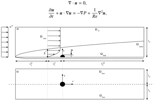
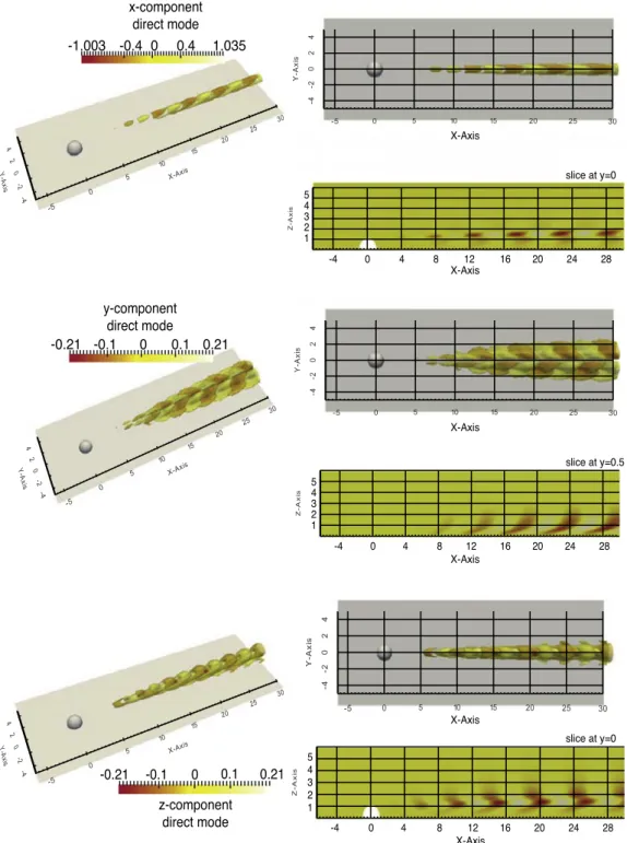
In the real world, however, we can observe flow configurations without any homogeneous spatial direction. The flow past a sphere (paper 7,10) or the flow over a hemispherical roughness element (paper 5) are exam-ples where the velocity and the pressure fields have strong variations in all

23 Theoretical framework

directions. In case of full 3D analysis, the normal mode ansatz is

q0(x, y, z, t) = 1

2{ˆq(x, y, z) exp[ t] + c.c.}. (2.18) We refer to Chapter 5 for further details about the numerical methods developed to solve such eigenvalue problems.

2.6

Zero-dimensional asymptotic analysis

In the previous sections, we used the translational invariance (local or two-dimensional analysis) or the scale separation (WKBJ) to reduce the full 3D stability equations to a lower dimensional problem. However, in several flow configurations, it is possible to consider a scale separation in all directions: this leads to a zero-dimensional asymptotic analysis. These techniques have originally been developed to study inviscid instabilities. In particular, we present the asymptotic theory developed by Bayly [17]. He proposed to adopt a short-wavelength approximation (WKBJ) to describe the evolution of the perturbations along closed streamlines. This approach is shortly outlined here; for a more detailed presentation the reader is referred to [18, 19]. The solution of the linearized Navier–Stokes equations is sought in the form of a rapidly oscillating and localized wave-packet, evolving along the Lagrangian trajectory X(t) and characterized by a wave-vector k(t) = r (X, t) and an envelope a(X, t) such that:

u(X, t) = ei (X,t)/✏a(X, t, ✏) = ei (X,t)/✏X n an(X, t)✏n (2.19) p(X, t) = ei (X,t)/✏b(X, t, ✏) = ei (X,t)/✏X n bn(X, t)✏n+1 (2.20)

where ✏ _{⌧ 1 and X = ✏x is a slowly varying variable. In the limit of} vanishing viscosity (Re _{! 1) and large wavenumbers (||k|| ! 1), the} theory provides the leading order term for the growth rate associated with a localized perturbation. This is obtained by integrating the following set of ordinary di↵erential equations

Dk Dt = H t_{(X)k, (2.21)} Da Dt = ✓ 2kkT |k|2 I ◆ H(X)a, (2.22)

24 Theoretical framework

along the Lagrangian trajectories defined by the ODE DX(t)

Dt = ub(X(t), t) . (2.23)

In the equations above_{H = ru}b is the base-flow velocity gradient tensor

and _{I the identity matrix. Since the flow under investigation is steady,} the Lagrangian trajectory corresponds to the streamlines of the base flow. Three initial conditions have to be assigned to solve the problem above: k(t = 0) = k0 , a(t = 0) = a0 and x(t = 0) = x0. The last condition

im-poses the Lagrangian origin of the streamline and thereby entirely identifies it.

Lifschitz & Hameiri [18] proved that a sufficient condition for inviscid instability is that the system of eqs. (2.21), (2.22) and (2.23) has at least one solution for which_{ka(t)k ! 1 as t ! 1. This theory has been} suc-cessfully applied in the past to study elliptic, hyperbolic and centrifugal instabilities of two-dimensional stationary base flows [20]. We apply this theory to characterize the instability mechanism arising inside an open cav-ity as discussed in paper 3. For this flow configuration, a central role is played by the closed Lagrangian trajectories (closed streamlines in paper 3), i.e. orbits described by material points which return to their initial po-sitions after a given time T (the period of revolution of a material particle). These closed trajectories play a special role in the dynamics of the instabil-ity: on the closed orbits, local instability waves propagate and feedback on themselves leading to a self-excited unstable mode.

As discussed above, the theory implies that both equations (2.21) and (2.22) must be integrated along these closed orbits. In the case investigated in paper 3, the base flow is steady and the streamlines are closed: eq. (2.21) is a linear ODE with periodic coefficients whose general solution can be written in terms of Floquet modes. In particular, the solution can be found by building the fundamental Floquet matrix _{M(T ), solution of the} system

D_M

Dt = H

t_{(X)M with M(0) = I , (2.24)}

and extracting its eigenvalues and the corresponding eigenvectors. Using these eigenvectors as initial conditions, it is possible to retrieve the tem-poral evolution of k during a lap around the closed streamline. Equation (2.21) admits three independent solutions related to the 3 eigenvectors of the fundamental Floquet matrix_{M(T ). In the case of two-dimensional base} flows, there exists for each orbit one eigenvalue equal to 1 with the corre-sponding eigenvector that remains constant in time and orthogonal to the

25 Theoretical framework

base flow. In other words, since the third column of _{H and the third line} of Ht _{are zero, the transverse component of k remains constant as time}

evolves. On the contrary, the in-plane components evolve under the action of the deformation tensor. Once equation (2.21) is solved, the amplitude a can be found by integrating equation (2.22). One can use any linear com-bination of the Floquet modes from equation (2.24) to set the specific k in equation (2.22).

Since we are trying to determine a self-excited mode, we need only to consider solutions of (2.21) that are periodic in time, i.e. solutions such that k(0) = k(T ). Here, as in Bayly [17], only eigenvectors orthogonal to the base flow are considered. With this choice, eq. (2.22) reduces to an ordinary linear di↵erential equation with periodic coefficients. According to Floquet theory, its solution can be written in terms of Floquet modes

a(t) = ¯a(t) exp( t) , (2.25)

where ¯a(t) is a periodic function (same period T as the material point moving along the selected closed streamline) and _{<{ } =} r is the growth

rate of the perturbation.

As for eq. (2.21), the fundamental Floquet matrix _{A corresponding to} equation (2.22) is built by integrating the system

D_A Dt = ✓ 2kkT |k|2 I ◆ H(X)A, (2.26) A(0) = I; (2.27)

along each orbit. The eigenvalues µi(x0) and the corresponding eigenvectors

of _{A(T ) can be easily extracted.}

As mentioned above, in case of two-dimensional base flows and in case in which the wavevector k is orthogonal to the x y plane, we expect one eigenvalue of _{A to be 1. The other two, for the incompressibility constrain,} must multiply to 1, i.e. µ1(x0) µ2(x0) = 1. The Floquet exponent (x0)

of the perturbation on the selected orbit 0 is obtained from the Floquet

multiplier µ(x0) of A by the simple relation

{n}₍ 0) = r( 0) + i {n}i ( 0) = log (µ) T ( 0) + i 2n⇡ T ( 0) with n2 N (2.28)

26 Theoretical framework

The growth rate of each WKBJ mode is simply given by the real part of

{n}_{. The frequency is related to the imaginary part and is not unique.}

Ac-cording to the formula (2.28), modes with the same growth rate (at leading order) but di↵erent frequencies are admissible: in particular the admissi-ble frequencies are integer multiple of the frequency of revolution along the same streamline.

Finally, in order to have a quantitative estimation of the leading eigen-value, we adopt the following formula proposed by Gallaire et al.[21]:

s = ( 0)

A k

k2

Re. (2.29)

They considered the viscous correction term [22] and the correction term relative to finite wavenumber e↵ects.

Chapter 3

Adjoint problem and

Structural sensitivity

3.1

Adjoint equations

The adjoint of a linear operator is a very powerful and useful concept in the field of functional analysis. The use of the adjoint in the context of hydrodynamic stability analysis has been recently reviewed by Luchini & Bottaro [28]. The adjoint solution can be used when one is looking for some outputs of a system for a large range of possible inputs. There are hundreds of applications of the adjoint in fluid mechanics like the receptivity of boundary layer flows or the identification of self-sustained thermoacoustic oscillations and a feedback mechanism efficient at suppressing them[29]. Furthermore, the adjoint is a fundamental tool in the control theory.

In the framework of hydrodynamic stability theory, the adjoint equations can be used to evaluate the e↵ects of a generic initial condition or forcing terms on the behaviour of the long time solution.

The derivation of the adjoint Navier-Stokes equations is based on the generalized Lagrange identity. Integrating over space and time such relation and using the divergence theorem provides the final system of equations that reads: @u† @t +L †_{u b, Re}u†+rP†= 0, (3.1) r · u†= 0, (3.2) 27

28 Adjoint field & Structural sensitivity

where _L† is the linear adjoint Navier-Stokes operator defined as:

L†{ub, Re}u†= ub· ru† rub· u†+

1 Rer

2_u† _(3.3)

In the present thesis we are interested in the global adjoint eigenmodes; thus, we express the adjoint perturbation field (u†_{, P}†_{) as a normal mode:}

q†(x, y, z, t) = ˆq†(x, y, z) exp{ t}. (3.4) Inserting (3.4) into equations (3.1-3.2) leads to an adjoint eigenvalue problem. Further details about the procedure adopted to obtain the adjoint system of equations (3.1-3.2) can be found in [35].

3.2

Classical sensitivity analysis

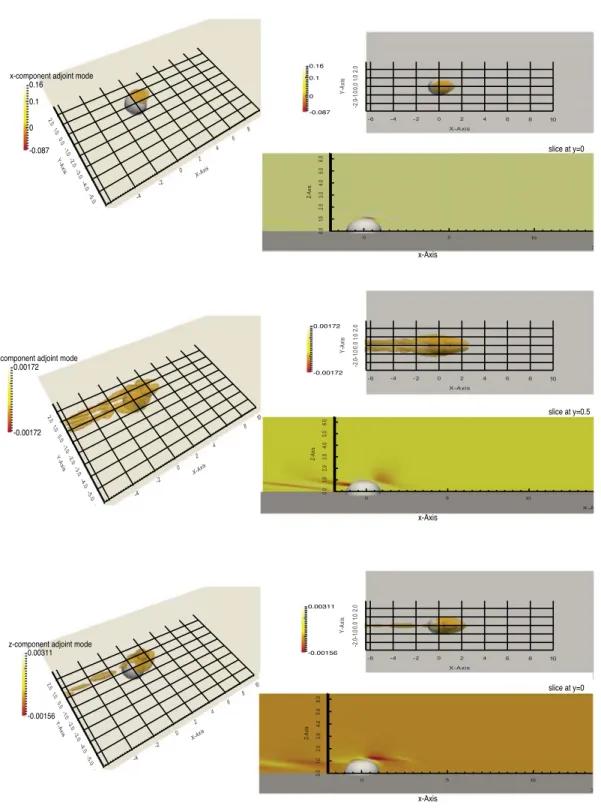
3.2.1 Structural sensitivity

The concept of structural sensitivity is general and can be applied to any dynamical system. Chomaz [31] investigated the stability features of the Ginzburg-Landau equation. He suggested to compute both direct and adjoint eigenvectors to determine the wavemaker region, i.e. the flow region giving rise to self-excited oscillations. Subsequently, Giannetti & Luchini [35] considered the flow past a circular cylinder. They underlined the large di↵erence existing between the spatial distribution of the direct global mode and the adjoint one due to the non-normality of the linearized Navier-Stokes operator. This fact suggests that the study of the direct global mode, with-out considering the adjoint field, cannot correctly identify the instability mechanism. Therefore, they performed a structural sensitivity analysis of the governing operator. In particular, the analysis focused on the varia-tions of the eigenvalue induced by a generic structural modification of this operator. The key idea of their approach is to model the feedback mecha-nism driving the instability by a local force proportional to the perturbation velocity which acts as a momentum source in the equations governing the evolution of the disturbance. This procedure leads to the definition of a new tensor defined as the product between the direct and adjoint fields:

S(x, y, z) = R ˆu†uˆ

Dˆu†· ˆudV

(3.5) A spatial map is then constructed by computing the spectral norm of this matrix. The function S(x, y, z) can be used to determine the locations

29 Adjoint field & Structural sensitivity

where the feedback is stronger, identifying in this way the regions where the instability mechanism acts.

This technique can take into account also strong non-parallel e↵ects and it can be adopted to investigate the instability mechanism of complex flows.

3.2.2 Sensitivity to base flow modifications

In an experimental set up a possible way to introduce a structural pertur-bation is to add a small obstacle in the flow field. As an example, Strykowski & Sreenivasan[32] discussed where the placement of a small cylindrical ob-stacle is able to delay the onset of vortex shedding in the wake of a circular cylinder. In their case, the presence of such obstacle produces both a modi-fication of the equations at the perturbation level and a modimodi-fication of the base flow.

The sensitivity analysis described in the previous section is based on a structural perturbation that acts only on the evolution of the perturbation field. This approach provides the right tool to investigate the wavemaker but does not take into account the structural perturbations that can act at the base-flow level. A generic perturbation, in fact, can induce also modifi-cations to the base flow that, in turn, produce changes in the coefficients of the linearized Navier-Stokes operator.

The so-called sensitivity to base flow variations is a concept introduced by Corbett et al.[33], and Marquet et al.[34]. In their analysis a small velocity-based perturbation can act at the base flow level: the e↵ect of the base flow modifications on the leading eigenvalue of the stability problem allowed them to study the di↵erent mechanisms that can suppress or en-hance the instability. The spatial structure of the so-called adjoint base flow [34] can be used to identify the features of the base flow that provide the main contribution to the instability dynamics and the regions where to locate e↵ective passive control devices.

This analysis leads to a definition of the tensor Sb which expresses the

sensitivity of the flow to base flow modifications:

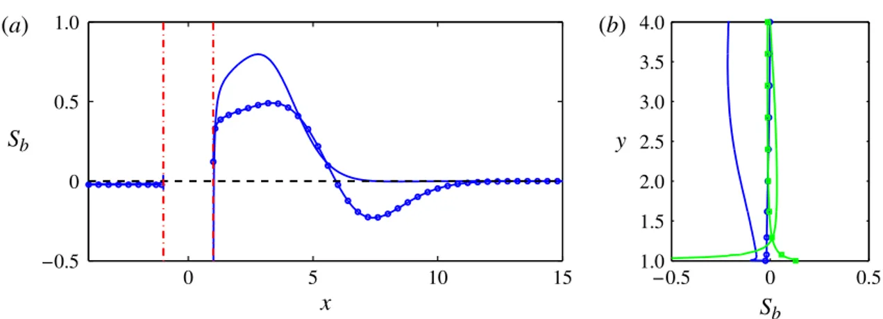
Sb= ˆ ub†ub R Duˆ†· ˆudV . (3.6)

As for the structural sensitivity, the spatial map can be obtained by selecting a suitable norm of Sb.

30 Adjoint field & Structural sensitivity

3.3

Second-order sensitivity

Sensitivity analysis has successfully located the most efficient regions in which to apply passive control in many globally unstable flows. As discussed in paper 2, the standard sensitivity analysis introduced in section (3.2.1) is linear with respect to the perturbation amplitude. Here, we introduce the second-order sensitivity analysis that allows us to predict also the e↵ect of steady spanwise wavy alternating modification on the flow stability. In fact, the standard analysis predicts that this kind of stationary wavy mod-ifications has no net e↵ect on the stability of planar flows. We generalize sensitivity analysis by including 2nd order terms in the computation of the eigenvalue drift.

We focus our attention on a generic eigenproblem of form:

Lˆq0 = 0ˆq0, (3.7)

whereL is the linearized Navier-Stokes operator, ˆq0a global linear temporal

eigenmode, and 0 = 0+ i!0 its eigenvalue. We now denote a structural

perturbation of the governing operator by _{L. Following Hinch[23], the} problem can be expanded in powers of the perturbation amplitude ✏:

(_{L + ✏ L) {ˆ}q0+ ✏ˆq1+ ✏2ˆq2+ O(✏3)} =

0+ ✏ 1+ ✏2 2+ O(✏3) {ˆq0+ ✏ˆq1+ ✏2ˆq2+ O(✏3)} (3.8)

Here, j is the jth order correction to the eigenvalue, and ˆqi (i > 0) is the

ith order correction to the eigenmode.

• At the 0th order in ✏, the original eigenvalue problem is recovered. • At the 1st _{order in ✏, we obtain, after rearrangement:}

(_L 0I) {ˆq1} = L{ˆq0} + 1ˆq0, (3.9)

where _{I is the identity operator. Equation (3.9) admits solution only} if a suitable compatibility condition is satisfied. This condition can be expressed through the adjoint eigenmode ˆq†₀, defined in Sec. 3 (see also [28]).

Such adjoint field ˆq†₀ satisfies the left eigenvalue problem. Thus, the product of the left hand side of (3.9) by ˆq†₀ vanishes. Hence, the right hand side also must be orthogonal to ˆq†₀(Fredholm alternative), giving 0 =hˆq†₀, L{ˆq0} + 1ˆq0i, which can be rearranged as:

31 Adjoint field & Structural sensitivity

This 1st _{order eigenvalue drift is a linear function of the operator}

perturbation, contains the direct and adjoint eigenmode, and lead to the standard sensitivity expressions (see section 3.2.1).

• At the 2nd _{order in ✏, we obtain from Eq. (3.8):}

(L 0I) {ˆq2} = L{ˆq1} + 2ˆq0+ 1qˆ1.

By the same argument as for the 1st _{order, both left and right sides}

are orthogonal to ˆq0, giving 2=hˆq†0, ( L 1I){ˆq1}i.

We observe that an arbitrary component of ˆq0can always be added to ˆq1

[23], and that Eq. (3.9) would still remain valid. Note that 2 remains

unaf-fected by the choice of this component, sincehˆq†₀, L{Cˆq0}i 1hˆq†₀, Cˆq0i =

0 for any constant C. The choice of C only corresponds to a normalization of the total perturbed eigenvector. A simple choice to guarantee uniqueness and remove the singularity of left-hand side in equation (3.9) is:

hˆq†₀, ˆq1i = C = 0, (3.11)

leading to:

2 =hˆq†0, L{ˆq1}i. (3.12)

Note that the 2nd order eigenvalue drift has exactly the same expression as the 1st order drift, but with the eigenmode ˆq0 replaced with the 1st order

eigenmode correction ˆq1. This means that all the sensitivity expressions

derived in the literature can be used straight away to obtain 2nd order corrections, if ˆq0 is replaced by ˆq1.

3.4

Inviscid Sensitivity analysis

There are several flow configurations in which it is possible to investi-gate the stability features by using the geometrical optics approximation. Physically, the resulting short-wave instabilities can be explained by local vorticity stretching. Three di↵erent types of instabilities exist: elliptic, hy-perbolic and centrifugal. These inviscid mechanisms were studied in detail by Sipp et al. [20], Godeferd et al.[36]. They focussed their attention on closed streamlines that play a special role in the dynamics of the insta-bility: on these orbits, local instability waves propagate and feedback on themselves leading to a self-excited unstable mode (see section 2.6 for the WKBJ analysis along the streamlines). In this context, our key idea is to isolate the e↵ect of the inviscid mechanism by increasing only the Reynolds

32 Adjoint field & Structural sensitivity

number in the global stability equations. In this way, we can use the result-ing inviscid structural sensitivity map to determine the flow regions where the inviscid mechanism acts. The resulting sensitivity tensor is function of both base-flow Reynolds number ReBF and the stability Reynolds number

ReST B:

S(ReBF, ReST B) = uˆ †_(u

b(ReBF); Re_RST B) ˆu(ub(ReBF); ReST B) Dˆu†· ˆudV

(3.13)

In paper 3, we showed that in the case of open cavity flow the resulting spatial map is very localized around a critical orbit inside the cavity. This orbit is the same identified by the WKBJ analysis and has a revolution period which is strictly related to the leading frequencies arising at higher Reynolds numbers.

3.5

Error Sensitivity to Refinement (ESR): an

in-dicator for optimal grid adaptation

The strategy we are going to describe is inspired by the structural sen-sitivity analysis introduced in section 3.2.1. A similar procedure, consisting in combining information between the direct and adjoint solutions, can also be used to derive an e↵ective indicator for grid refinement strategies. Grid refinement is a powerful tool that can be used in intensive and memory demanding applications to reduce the computational costs and, at the same time, retain and even improve the accuracy of the numerical problem. Re-ducing both errors and costs in a numerical simulation is a general and fundamental problem in computational sciences and is strictly related to uncertainty quantifications analysis. Further details about the proposed approach can be found in paper 9.

We focus our attention on a di↵erential problem on a domain ⌦ with given b.c. on @⌦. Let’s consider an algebraic operator Nhobtained through

a discretization of the continuous problem on a mesh with characteristic spacing h. If uh is a solution of the discrete problem then

Nh(uh) = 0 (3.14)

while the exact solution of the continuous problem uex satisfies

33 Adjoint field & Structural sensitivity

where the term rh is named residual. We measure the error between the

approximate and exact solution using the E2 definition of the error:

E2= ✓Z ⌦|u ex(x) u(x)|2dS ◆1/2 . (3.16)

Replacing the integral by its numerical approximation, we can express the equation (3.16) as:

E₂2 =X

i

wi(uh,i uex,i)2 (3.17)

where wi are suitable weights composing a numerical quadrature formula.

We want now to determine the sensitivity of the error E2to a small variation

in the residual rh (its gradient vh), or in other terms the gradient of E2

with respect to rh.

A small variation uh in the numerical solution uh produces a variation

in the error of the form:

E2 E2= y · uh (3.18)

where y is the vector with components yi = wi(uh,i uex,i). By applying

the adjoint analysis, we now write E2 as a linear function of the residual.

In order to achieve this, we first note that a small variation in the solution produces a small change in the residual according to

A uh = rh (3.19)

where A = @Nh

@u is the Jacobian of the di↵erential operator in (3.14). By

multiplying (3.19) by a vector vh and using the definition of the adjoint

operator we can write

vh· Ah uh= uh· AThvh= vh· rh (3.20)

If we now choose the adjoint vector vh such to satisfy

AT_h vh = y/E2 (3.21)

we can rewrite the variation of the error in terms of a small residual change as

E2 E2 = y· uh = E2vh· Ah uh= E2vh· rh. (3.22)

Assume now that, asymptotically for small h, rh ⇠ hp for some integer

exponent p (the order of the discretization). A variation in h (a grid refine-ment) by a factor m (say 1/2) will then induce a variation in the residual proportional (with opposite sign) to the residual itself, i.e.

34 Adjoint field & Structural sensitivity

This is, in fact, the rationale behind recovery-based methods: refining where the residual is largest produces the maximum reduction in the residual. We may also notice that, when the residual is related to the truncation error of a di↵erential operator, the relationship between residual and refinement is a local one.

Such relation is still not what we really look for: in fact our aim is to know what happens when we refine the grid, which is not the same as changing the residual. To get the complete answer to our problem we need to consider what happens to the residual when we refine the grid.

Recalling now that the spatial map of the residuals indicates where a local refinement will mostly decrease the residual itself. On the other hand, the spatial map of the adjoint provides information on the location where a change in the residual will mostly a↵ect the error. These two quantities can be compared with the direct and adjoint solution of the structural sensitiv-ity analysis for fluid flow problems with self-exciting instabilities discussed above. As for those cases, we can now make a step forward and combine the information provided by the two maps by taking the local product between the residual and the adjoint field. In this way we define the Error Sensitivity to Refinement (ESR)

si= E22vh,irh,i (3.24)

where no implicit summation is assumed. This quantity indicates where a local refinement (by a fixed factor m) will mostly a↵ect the error E2 and it

is therefore a natural indicator to really minimize (3.16). In general, both error and residual require a knowledge of the exact solution. Just as for all the other mesh-adaptation indicators, the latter can be estimated and replaced by a solution on a finer mesh. In particular, if both the error and the residual asymptotically decrease like hp_{, we obtain the following relation}

u2h uh ' (1 2 p)(u2h uex)' (2p 1)(uh uex) (3.25)

between the error on grid h and the error of the solution with respect to a finer grid. Furthermore, considering that u2h is the discrete solution on the

course mesh, it is also possible to write

N2h(uh) N2h(u2h) | {z } =0 ' (1 2 p)(N2h(uex) N2h(u2h) | {z } =0 )' (2p 1)Nh(uex) (3.26)

which gives an estimate of the residual using the solution on a finer mesh. As a final remark we note that the error sensitivity si = E22vh,irh,i tends

35 Adjoint field & Structural sensitivity

to a grid-independent limit for h _{! 0 so that sensitivity maps obtained} on di↵erent grids will be similar provided the mesh spacing h is sufficiently small.

Chapter 4

Stabilization of the solution

of the Navier-Stokes

equations

The solution of the Navier-Stokes equations can change from stable to unstable with a variation of a control parameter. A classical example of such process is the instability occurring in the wake of a circular cylinder: at low Reynolds number, i.e. for Re < 46.7, the flow is steady and symmetric, but for larger values of Re a global instability arises in the flow field lead-ing to the well-known von K´arm´an vortex street [35]. In order to perform stability computations beyond the critical threshold we need a numerical method able to track the base flow across and beyond the critical point. Unfortunately, we cannot use a standard time integration of the governing equations just because it is unstable.

The discretization of the governing equations, especially for fluid dynamic applications, often leads to very large discrete systems. As a consequence, matrix based methods, like for example the Newton-Raphson algorithm cou-pled with a direct inversion of the Jacobian matrix, lead to computational costs too large in terms of both memory and execution time.

In the case of high-dimensional systems, few computations have been performed in the literature. The most popular method to stabilize an un-stable procedure was proposed by Shro↵ & Keller[37]. Their Recursive Projection Method (RPM) stabilizes an unstable algorithm by using the Newton method only on a small subspace. Another popular stabilization algorithm was presented by Akervik et al.[38]. The details of both methods will be provided in section 4.2 and 4.3 respectively. However, these methods

38 Stabilization of the solution of the Navier-Stokes equations

present some drawbacks.

A new stabilization algorithm is proposed in paper 8. This method, named BoostConv, can stabilize a pre-existing numerical procedure used to integrate any dynamical system without negatively impacting on its compu-tation time. Moreover, it can be easily inserted in the pre-existing relaxation (integration) procedure with a call to a single black-box subroutine.

4.1

Iterative solution of a linear system

The study of a dynamical system described by a set of partial di↵erential equations (PDEs) usually involves the solution of a linear system:

Ax = b, (4.1)

where A is aRN⇥N matrix and x, b areRN vectors representing respectively the solution and the known term of the system. A generic linear iteration for the solution of the linear system (4.1) can be expressed as:

xn+1= (I BA)xn+ Bb = xn+ Brn. (4.2)

In the previous expression rn = b Axn is the residual and B is a matrix

representing the particular iterative scheme used to solve the problem (see e.g. Ch.4 [39]). The convergence of procedure (4.2) is governed by the eigenvalues of the iteration matrix M = I BA: the algorithm converges if and only if the spectral radius of the iteration matrix is less than 1. The asymptotic convergence rate is essentially governed by the slowly decaying modes.

4.2

The Recursive Projection Method (RPM)

The recursive projection method was initially developed for extending the domain of convergence of iterative procedures in the context of stability and bifurcation analysis. As discussed above, the convergence of a generic iterative procedure (4.2) is related to the eigenvalues of M. In order to illustrate the RPM method, we suppose that the iteration (4.2) diverges be-cause of s unstable eigenvalues. Shro↵ & Keller introduced a small subspace P 2 Rs spanned by the eigenvectors associated with the unstable eigenval-ues (i.e. the eigenvaleigenval-ues that have a modulus larger than 1) and _{Q that is} the orthogonal complement of the former subspace. Thus, the sum between these two spaces provides the whole RN: xT OT = xp+ xq. The projectors

39 Stabilization of the solution of the Navier-Stokes equations

˜

P and ˜Q associated to _{P and Q can be defined by an orthonormal basis ˜}V for P as:

˜

P = ˜V ˜VT, Q = I˜ V ˜˜VT, (4.3) where superscript T represents the transpose operator.

The resulting RMP procedure can be written as follows:

xn+1_q = ˜Q [Mxn+ Bb] ; (4.4)

xn+1_p = xn_p + (I P M ˜˜ P ) 1{ ˜P [Mxn+ Bb] xnp}; (4.5)

xn+1= xn+1_p + xn+1_q . (4.6)

Thus, at each step, only the projection of equation (4.2) onto the sub-space Q is solved with the original iteration. The iteration on the low-dimensional subspace _{P is solved with Newton’s method. Shro↵ & Keller} [37] discussed the e↵ectiveness of the algorithm proving the e↵ective con-vergence even in case of unstable procedures. However, the RPM can be inefficient in the case of large linear systems due to the existence of modes with large negative real parts. In such cases, the resulting asymptotic con-vergence rate of the RPM algorithm is reduced.

4.3

SFD

Akervik et al.[38] presented the Selective Frequency Damping method. They showed that an existing time integration procedure for the solution of N-S problem, can be coupled with the SFD algorithm to reach a steady state by damping the unstable temporal frequencies. This is achieved by adding a dissipative relaxation term proportional to the high-frequency content of the velocity fluctuations. Here, we briefly describe the method; we refer to the original paper [38] for further details.

Let us consider a generic non-linear dynamical system, e.g. the Navier-Stokes system, that reads:

@

@tq = L{q}, (4.7)

where q is the state of the system and L is the di↵erential operator. The key idea of the SFD algorithm is to add to the right-hand side a linear term forcing towards a target solution ˜q: (q q). Here, the coefficient˜ represents the amplitude of the control. Since the target solution is not available, they decided to approximate ˜q as a modification of the current state q but with reduced temporal fluctuations. Thus, to obtain this aim,

40 Stabilization of the solution of the Navier-Stokes equations

the target solution is obtained as ˜q = T_{⇤ q, where T is the temporal filter} kernel; i.e. they adopted a temporal low-pass filter on q. The resulting modified dynamical system reads:

@

@tq = L{q} (I T)⇤ q, (4.8)

where I is the identity operator. Note that if q = qs, the forcing term

vanishes. The computed steady state of (4.8) is also a solution of the original problem. However, the SFD algorithm needs an estimate of the global mode frequency and it cannot be applied to compute unstable states in presence of stationary bifurcations.

4.4

BoostConv

The aim of the present section is to present a new algorithm, inspired by Krylov-subspace methods, able to compute efficiently such unstable states of a high-dimensional dynamical system. This method is based on the min-imization of the norm of the residual at each integration step and can be applied as a black-box procedure in any iterative or time marching algo-rithm without negatively impacting the computational time of the original code.

The main idea which inspired the proposed algorithm is similar to the one at the basis of GMRES[39], but in a reverse logic sequence. We start from an existing iterative algorithm that is modified to Boost the Conver-gence of the overall procedure.

To obtain this stabilization, we focus our attention on the evolution of the residual. We can simply obtain the homogeneous equation for the propagation of the residual by applying A to (4.2) and successively adding b:

b Axn+1= b A [xn+ B(b Axn)] , i.e.

rn+1= rn ABrn. (4.9)

Now, in order to improve the existing procedure (4.2), we replace the residual vector rnwith a modified residual ⇠n such that the improved

algo-rithm reads

xn+1= xn+ B⇠n(rn). (4.10)

In the previous equation ⇠_n is a suitable function of rn and can be

41 Stabilization of the solution of the Navier-Stokes equations

perturbation to the original iteration matrix. We note that to guarantee the consistence of the modified algorithm, it is sufficient that ⇠_n goes to zero when rn does. The introduction of the vector ⇠n modifies equation (4.9)

leading to the new residual equation

rn+1= rn AB⇠n, (4.11)

or equivalently

rn rn+1= AB⇠n. (4.12)

We now minimize rn+1 by choosing a suitable function ⇠n = ⇠n(rn). If we

knew (AB) 1_{, we could exactly annihilate r}

n+1 by computing ⇠n(rn) as

⇠_n= (AB) 1rn. (4.13)

However, for large systems, the exact inversion of AB is out of reach or too expensive to be performed. Therefore, we approximate the solution of (4.13) by using a classical least-square method.

The action of the operator AB can be represented by storing a set of N vector pairs (ui, vi), where the second member is produced by the action of

AB on the first. Least-squares method is then adopted to approximate the solution of the algebraic linear system AB⇠_n= rn as

⇠_n=

N

X

i=1

ciui. (4.14)

In our case the vectors ui and vi are related by

vi= ABui for i = 1, .., N. (4.15)

while the coefficients ciare chosen to minimize|rn AB⇠n|2. The standard

least-squares procedure leads to a system of equations for the coefficients ci

of the form

Dklcl= tk (4.16)

where tk = vk· rn and Dkl = vk· vl is a small N ⇥ N matrix. Matrix D

is usually ill-conditioned and an orthogonalization procedure (QR decom-position) is usually needed to find the solution. However, when N is small, as for the cases we are considering, the solution can be simply found with a classical LU decomposition. This least-square solution is not exact and produces a residual ⇢ = rn AB⇠n which can be expressed in terms of vi

42 Stabilization of the solution of the Navier-Stokes equations ⇢ = rn AB⇠n = rn AB N X i=1 ciui ! = rn N X i=1 ciABui = rn N X i=1 civi. (4.17) However, inserting the so calculated ⇠_n in (4.10) is not yet sufficient to produce a converging algorithm because ⇠_ncould converge to zero even when the residual rn is not identically zero, but simply orthogonal to the leading

N (basis-)vectors ui. Remembering that the original iterative algorithm

(4.2) simply had ⇠_n= rn, we restore a convergent procedure by adding the

residual ⇢ = rn Picivi to ⇠n, so that the complete algorithm now reads

⇠_n=X i ciui+ rn X i civi (4.18)

The rationale behind this procedure is to invert exactly the part of the problem represented by the dominant, slower decaying modes, while letting the original iterative algorithm to handle the remaining modes. We now go back to the issue of selecting a convenient set of vectors ui. In the case

of BoostConv, both ui and vi can be conveniently calculated by observing

that, according to (4.11), for each n we have

rn rn+1= AB⇠n. (4.19)

For a given N, in a cyclic fashion, at the beginning of a new iteration, we add a new vector pair by selecting uN = ⇠n 1 and vN = rn rn 1. In

order to keep the size of the basis constant, another pair must be discarded which typically will be the oldest. Such choice is dictated by the fact that applying the algorithm to a nonlinear system it is beneficial to use the freshest information on the system dynamics in order to account for the change of the system Jacobian (in our case represented by the linear operator A). We also note that in matrix Dkl of (4.16) only the row and the column

involving a new pair need to be updated. Such selection procedure works when we already have N vector pairs. At the beginning of the algorithm (for n < N ) we can still use the same procedure but continuously increasing the basis dimension from 1 to the chosen value of N . In this first stage, no vector pairs are discharged.

From a programming viewpoint, the BoostConv algorithm can be en-capsulated in a black-box procedure, where the only input is rn and the

only output is ⇠_n. If ⇠_n is returned in the same vector where rn was

pre-43 Stabilization of the solution of the Navier-Stokes equations

existing iterative algorithm (4.2) is a single line of code containing the call to BoostConv.

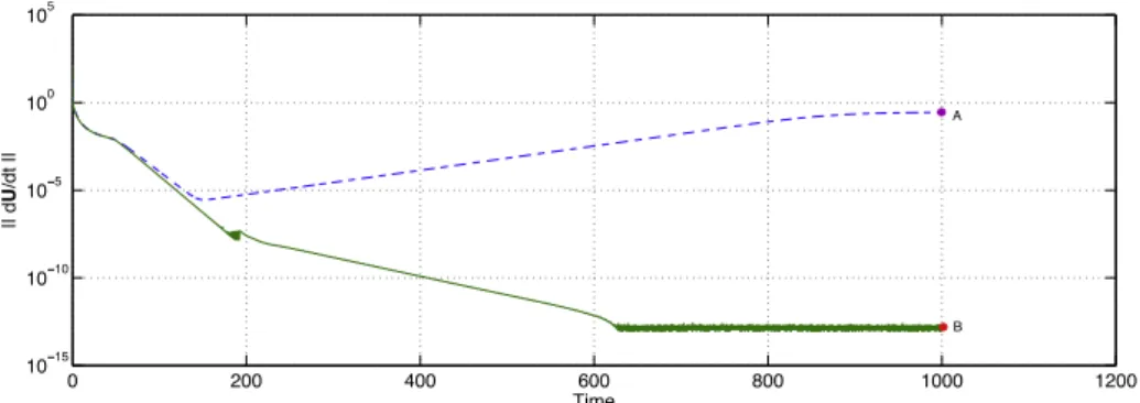
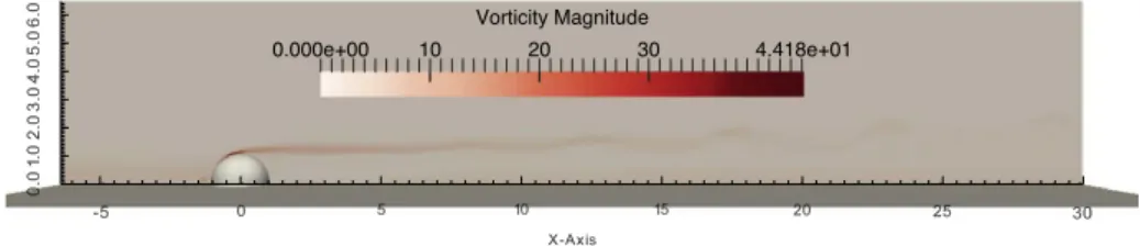
In paper 8, we report numerical results obtained with this new proce-dure. We started from the classical case of the two-dimensional lid-driven cavity flow where we show that BoostConv is able to accelerate the con-vergence of the existing time integration procedure. Then, we consider the case of the two-dimensional flow past an infinitely long circular cylinder. For this case, we show, with several di↵erent codes, that BoostConv is able to drive the iterative procedure to the exact base flow (computed using a Newton method). A three-dimensional case is also considered to examine the application of BoostConv to a high-dimensional problem. In particular, we discuss the results obtained from the application of BoostConv to the case of boundary layer flow past a hemisphere reported in paper 5. In this case we checked also that the whole algorithm (time integration by us-ing Nek5000+ BoostConv) has a computational burden very similar to the original iteration.

Chapter 5

Numerical methods

In the present thesis, three di↵erent codes have been used to perform the stability analyses presented in the papers (pert II). In the following, we briefly describe each approach, further details about F reef em++ can be found in [40]; for N ek5000 we refer to [44] while the multigrid code is described in paper 7.

5.1

F reef em++

F reef em++ is a free software based on the Finite Element Method; it has its own high level programming language. It has been adopted to investigate many phenomena involving di↵erent systems of PDE like e.g. fluid-structure interactions, Lorentz forces for aluminum casting and ocean-atmosphere coupling. We used this software to solve both the base flow problem and the stability eigenvalue problems.

5.1.1 Base flow

The variational formulation of the Navier-Stokes equations is derived. We used the classical P 2 P 1 Taylor-Hood elements for the spatial dis-cretization. The resultant nonlinear system of algebraic equations, along with the boundary conditions, is solved by a Newton-Raphson procedure: given an initial guess wb(0), the linear system

NS(Re, Wb(n))· wb(n)= rhs(n) (5.1)

is solved at each iteration step using the MUMPS-Multifrontal Massively Parallel sparse direct Solver [41] for the matrix inversion. The base flow is

46 Numerical methods

Mesh σ ! nd.o.f. nt Source

M1 0.0007590 7.4931 998668 221045 Present

M2 0.0008344 7.4937 1416630 313791 Present

M3 0.0009122 7.4943 2601757 576887 Present

D1 0.0007401 7.4930 880495 194771 [45]

D2 0.0008961 7.4942 1888003 418330 [45]

Table 5.1: Comparison of the results obtained with the present F reeF em++ code and those reported by [45] for the flow over an open cavity. The eigenfrequency ! and the growth rate have been calculated for the first two-dimensional unstable eigenmode at Re = 4140. nd.o.f. and

ntindicate the total number of degrees of freedom of the linearized problem

and the number of triangles for each of the unstructured meshes used.

then updated as

Wb(n+1)= Wb(n)+ wb(n). (5.2)

The initial guess is usually chosen to be the solution of the Stokes equations and the process is continued until the L2_{-norm of the residual of the}

gov-erning equations becomes smaller than a given tolerance. The tests about the convergence of the resulting code has been performed for the case of the open cavity. We used three di↵erent meshes _{M1, M2 and M3 (see} Table 5.1). These are generated by the Bidimensional Anisotropic Mesh Generator (Bamg) that is part of the Freefem++ package. The base flow computations are also validated using a variant of the second-order finite-di↵erence code described in [35].

5.1.2 Direct and Adjoint eigenvalue solver

Once the base flow is determined, the system of equations (2.16) is used to perform the stability analysis. After spatial discretization, the governing equations and their boundary conditions are recast in the following standard form

[A(Re, Wb(Re)) + B]· w = 0, (5.3)

where w is the right (or direct) eigenvector. As methods based on the QR decomposition are not feasible for solving large scale problems as those associated to the matrix A obtained for our problem, we adopt an efficient matrix-free iterative method based on the Arnoldi algorithm [42] . We use the state-of-the-art ARPACK package [43], with implicit restarts to limit

47 Numerical methods

memory requirements. The solution of the linear system built by the Arnoldi iterations on the Krylov subspace is obtained with the same sparse solver [41] used for the base flow calculations. The adjoint modes are computed as left eigenvectors of the discrete system derived from the discretization of the linearized equations and the sensitivity function is then computed by the product of the direct and the adjoint fields.

The code is validated against the results reported by [45]. These authors investigate the stability of a newtonian fluid in the same geometrical con-figuration of paper 3 and report the first instability of a two-dimensional eigenmode to occur at Re=4140. In Table 5.1 we present the comparison between our results and the results in [45] for di↵erent meshes. In these tests, 50 eigenvalues were obtained, with an initial Krylov basis of dimen-sion 150; the convergence criterion for the Arnoldi iterations is based on a tolerance of 10 9_{. To independently check the accuracy of the results we a}

posteriori computed the residual maxi|(Aij+ Bij)wj|: this turns out to be

always below 10 9 for the results reported in this paper, typically less than 10 12 _{for the least stable modes.}

5.2

N ek5000

N ek5000 is a computer software used to simulate fluid flow and heat transfer for steady and unsteady two-dimensional and three-dimensional ge-ometries. The code includes: i) P REN EK as a pre-processor; ii) N EKT ON as solver and iii) P OST N EK as a post processor. P REN EK is a prepro-cessor in which is possible to specify the mesh and the boundary and initial conditions. N EKT ON is a parallel spectral element solver that computes the velocity and pressure fields. These results can then be analyzed in the post processor P OST N EK. The code is written in f77 and the paralleliza-tion is achieved by using the MPI interfaces.

N ek5000 is based upon the spectral element method [46] which combines the high-order accuracy of spectral methods with the geometric flexibility of traditional finite-element methods.

The computational domain is divided into non-overlapping quadran-gles; the unknown is approximated by high-order polynomial expansions. In particular, the unknown vector (u, v, w, P ) is spatially discretized onto PN PN 2spectral elements using Lagrange orthogonal polynomials in the

Gauss-Lobatto-Legendre (GLL) nodes. For the temporal discretization of momentum equation, a semi-implicit splitting scheme has been used because it allows high-order temporal accuracy. The time advancement is divided in 3 independent subproblems: convective, viscous, and pressure problem.