Accoppiamento di codici CFD e codici di
sistema in sistemi a piscina ed a loop
G. Barone, N. Forgione, D. Martelli, W. Ambrosini
Agenzia nazionale per le nuove tecnologie,
ACCOPPIAMENTO DI CODICI CFD E CODICI DI SISTEMA IN SISTEMI A PISCINA ED A LOOP
G. Barone, N. Forgione, D. Martelli, W. Ambrosini (UNIPI)
Settembre 2013
Report Ricerca di Sistema Elettrico
Accordo di Programma Ministero dello Sviluppo Economico -‐ ENEA Piano Annuale di Realizzazione 2012
Area: Produzione di energia elettrica e protezione dell'ambiente
Progetto: Sviluppo competenze scientifiche nel campo della sicurezza nucleare e collaborazione ai programmi internazionali per il nucleare di IV Generazione
Obiettivo: Sviluppo competenze scientifiche nel campo della sicurezza nucleare Responsabile del Progetto: Mariano Tarantino, ENEA
Il presente documento descrive le attività di ricerca svolte all’interno dell’Accordo di collaborazione “Sviluppo competenze scientifiche nel campo della sicurezza nucleare e collaborazione ai programmi internazionali per il nucleare di IV generazione” Responsabile scientifico ENEA: Mariano Tarantino
Lavoro svolto in esecuzione dell’Attività LP2.C1_e
UNIVERSITA’ DI PISA
DICI
System codes and a CFD codes applied to loop- and
pool-type experimental facilities
(Accoppiamento di codici CFD e codici di sistema in sistemi a
piscina ed a loop)
G. Barone, N. Forgione, D. Martelli, W. Ambrosini
CERSE-UNIPI RL 1530/2013
Summary
This report, carried out at the DICI (Dipartimento di Ingegneria Civile e Industriale) of Pisa University in collaboration with ENEA Brasimone Research Centre, deals with the modification of the relationship used by the RELAP5 system code to generate the table of LBE, Lead and Sodium and with post-test thermo-fluidynamic analyses of NACIE loop type (Natural Circulation Experiment) facility and of CIRCE-DHR (Circulation Eutectic- Decay Heat Removal System) pool type facility, built at ENEA. Experimental results are compared with those obtained from RELAP5 stand alone calculations and from RELAP5-FLUENT coupled code calculations.
In particular, in the first part of this work the equations were modified into RELAP5/Mod3.3 system code to obtain the thermodynamic properties of lead, LBE and sodium and are presented for both saturation and single phase conditions.
The second part of this work deals with post-test analyses of the NACIE loop type facility: computational results are obtained both from RELAP5 stand alone and from an in-house coupling tool achieved using RELAP5 thermal-hydraulic system code and CFD Fluent commercial CFD code.
After that, a post-test simulation reproducing an accidental event with a total loss of the secondary circuit followed by a reactor scram and DHR system activation to remove residual heat generation, was performed using the RELAP5 code on Test IV of CIRCE facility experiments.
Comparative analyses among the simulations performed by RELAP5-Fluent coupled codes and by RELAP5 stand-alone code agreed well, moreover results obtained for the CIRCE-DHR demonstrate the RELAP5 model’s suitability in simulating a PLOH+LOF transient representative experiment.
Index
Summary ... .2
1. Thermodynamic properties used to generate RELAP5 tables for
LBE, lead and sodium ... 5
1.1 Liquid phase ... 5
1.1.1 Saturated vapor pressure ... 5
1.1.2 Saturated vapor temperature ... 5
1.1.3 Specific volume at atmospheric pressure ... 5
1.1.4 Specific heat at atmospheric pressure ... 6
1.1.5 Derivative obtained using approximate correlation only function of temperature ... 6
1.1.6 Specific volume as a function of temperature and pressure ... 6
1.1.7 Isobaric coefficient of thermal expansion ... 7
1.1.8 Isothermal coefficient of compressibility ... 7
1.1.9 Specific enthalpy ... 7
1.1.10 Specific entropy ... 8
1.2 Vapour phase ... 9
1.2.1 Specific volume ... 9
1.2.2 Isobaric coefficient of thermal expansion ... 9
1.2.3 Isothermal coefficient of compressibility ... 9
1.2.4 Specific heat at constant volume ... 9
1.2.5 Specific heat at constant pressure ... 9
1.2.6 Specific internal energy ... 9
1.2.7 Specific entropy ... 10
2. Correlations for LMs implemented inside the RELAP5 code ... 11
2.1 Transport properties ... 11
2.2 Convective heat transfer correlations ... 11
3. Description of the NACIE loop facility ... 13
4. NACIE experimental campaign ... 17
5.1 RELAP5 Model ... 18
5.2 RELAP5 Post-Test Simulations... 19
6 RELAP5-Fluent coupled calculations ... 27
6.1 RELAP5 and Fluent models ... 27
6.2 Coupling procedure ... 30
6.3 Matrix of simulations ... 31
6.4 Obtained results: Test 206 and Test 306 ... 32
7 Thermal-hydraulic post-test analysis of ICE-DHR ... 38
7.1 Post-Test RELAP5 simulations ... 38
7.2 Test IV. Initial and Boundary Conditions ... 40
7.3 Test IV. PLOH+LOF Simulation Analysis ... 41
8. Conclusions ... 46
References ... 47
Nomenclature ... 48
1. Thermodynamic properties used to generate RELAP5 tables for
LBE, lead and sodium
In this section the equations needed to obtain temperature, pressure, specific volume, specific internal energy, thermal expansion coefficient, isothermal compressibility, specific heat at constant pressure and specific entropy are presented for both saturation and single phase conditions. The thermodynamic properties of lead, LBE and sodium have been found in V. Sobolev's work [1]. Properties and coefficients used inside the correlations, where not specified, are reported in SI base units.
1.1
Liquid phase
1.1.1 Saturated vapor pressure
Sobolev [1] reports the following correlation for the saturation pressure as a function of temperature.
( )
2 1 exp sat a p T a T = ⋅
(1.1)where for LBE is a1=1.22E10 and a2= -22552 and for lead a1=5.76E9 and a2= -22131. For sodium, the saturation pressure was reported in a more complicated form by Sobolev, but starting from it and using a better fitting method a correlation with the same form used for LBE and lead is derived. In particular, for sodium the two previous coefficients are found to be: a1=4.18965E9 and a2= -1.22805E4.
1.1.2 Saturated vapour temperature
As a consequence of the previous correlations, temperature can be written as a function of pressure through the following equation:
( )
2 1 ln sat a T p p a = (1.2)1.1.3 Specific volume at atmospheric pressure
From Sobolev's work density at atmospheric pressure (pref 10 5
Pa) is given as the following linear function of temperature:
( )
, 0 1
l ref T r r T
ρ = + (1.3)
In the present work the use of polynomial form for the specific volume correlation is preferred. Then, using a least-squares regression method, the Sobolev correlation for density was transformed in the following form:
( )
2 3 , 0 1 2 3 l ref v T =b +b T+b T +b T (1.4) whereb0=9.02805304E-05, b1=1.09001277E-08, b2=8.44153423E-13, b3=3.10620231E-16 for LBE; b0=8.73593582E-05, b1=9.93870088E-09, b2=8.88207610E-13, b3=2.24367865E-16 for lead; b0=9.80671847E-04; b1=2.54530643E-07; b2=1.23725177E-11; b3=3.59886201E-14 for sodium.
1.1.4 Specific heat at atmospheric pressure
The correlation for the specific heat at atmospheric pressure (pref 10 5
Pa) is given by Sobolev, as a function of temperature, in the form:
( )
2 2, 0 1 2 3
p l ref
c T =e +e T+e T +e T− (1.5)
In the present work the use of a third order polynomial of temperature is preferred. Then, using a regression method, the Sobolev correlation was here transformed in the following form:
( )
2 3, 0 1 2 3
pl ref
c T =d +d T+d T +d T (1.6)
where
d0=1.57972755E+02, d1=-2.47822044E-02, d2=1.72861218E-06, d3=2.60782635E-09 for LBE; d0=1.61791750E+02, d1=-2.31399817E-02, d2=-1.45020777E-06, d3=3.70731445E-09 for lead; d0=1.60476754E+03, d1=-7.22160215E-01, d2=3.41613663E-04, d3=2.86782393E-08 for sodium.
1.1.5 Derivative obtained using approximate correlation only function of
temperature
Assuming the enthalpy derivatives only as function of temperature, they can be calculated using the correlation for the specific volume given at reference pressure:
, 2 3 , 0 2 3 2 2 , 2 3 2 2 2 2 2 6 l ref l l l l ref p T l ref l l T p p dv h v v T v T b b T b T p T dT d v h v T T b T b T T p T dT ∂ = − ∂ ≅ − = − − ∂ ∂ ∂ ∂ ∂ = − ≅ − = − − ∂ ∂ ∂
(1.7)1.1.6 Specific volume as a function of temperature and pressure
Since the specific volume is a function of temperature and a weak function of pressure the first two terms of the Taylor series can be used to obtain this dependence:
(
,)
,( )
(
)
l l l ref ref T v v T p v T p p p ∂ ≅ + − ∂
( )
( )
, , l l ref l ref T v v T T p κ ∂ ≅ − ∂
(
,)
,( )
,( )
,( )
(
)
l l ref l ref l ref refv T p ≅v T −v T κ T p−p (1.8)
, ,
s l pl ref
w c
where
c0=2.96266725E-11, c1=7.63414010E-15, c2=1.33519112E-17 for LBE;
c0=2.48689008E-11, c1=9.28978837E-15, c2=1.06789185E-17 for lead;
c0=1.93389526E-10, c1=-7.87675461E-14, c2=2.45166675E-16 for sodium.
1.1.7 Isobaric coefficient of thermal expansion
The thermal expansion coefficient was approximated by the following equation:
(
)
(
1)
,(
1 2 2(
3)
3 2)
, , , l ref l l l b b T b T dv T p v T p dT v T p β ≅ = + + (1.11)1.1.8 Isothermal coefficient of compressibility
The isothermal coefficient of compressibility was evaluated through:
(
)
,( )
(
,)
( )
( )
,( )
(
)
, ,
, 1
l ref l ref l ref
l l l ref ref v T T T T p v T p T p p κ κ κ κ ≅ = − − (1.12) and then
(
)
(
0 1 2)
(
2)
2 0 1 2 , 1 l ref c c T c T T p c c T c T p p κ = + + − + + − (1.13)1.1.9 Specific enthalpy
The specific enthalpy can be written, in the same way as performed for the specific volume, i.e.:
(
,)
,( )
(
)
l l l ref ref T h h T p h T p p p ∂ ≅ + − ∂
(1.14)Integrating first between a reference temperature Tref and the generic temperature T for p=pref and after between pref and p along T=const we obtain:
(
,)
0 ,( )
ref ref T p l l l pl ref T p T h h T p h c T dT dp p ∂ = + + ∂
∫
∫
(1.15) and then( )
(
)
1(
2 2) (
2 3 3) (
3 4 4) (
2 3)
(
)
0 0 0 2 3 , 2 2 3 4l l ref ref ref ref ref
d
d d
h T p =h +d T T− + T −T + T −T + T −T + b −b T − b T p−p (1.16)
The latent heat of melting is about 38600 J/kg for LBE, 23070 J/kg for lead and 113000 J/kg for sodium, while the specific heat for the solid phase is about 128, 127 and 1234 J/(kg K), respectively. Choosing the value of 273.15 K as reference temperature and assuming the specific enthalpy equal to zero, one can be obtain:
(
)
0 , 0
l p solid melt melt
h =c T −T + ∆h (1.17)
with Tref = Tmelt and pref =10 5
Pa.
(
,)
,( )
(
)
l l pl pl ref ref p T p h h c T p c T p p T T p ∂ ∂ ∂ ≡ = + − ∂ ∂ ∂ (1.18) with 2 2 , 2 2 l ref l l T p p d v h v T T T p T dT ∂ ∂ ∂ = − ≅ − ∂ ∂ ∂ (1.19) Then(
)
( )
2 ,(
)
, 2 , l ref p l p l ref ref d v c T p c T T p p dT = − − (1.20)and using the derivative of specific volume one is obtains:
(
)
2 3(
2)
(
)
0 1 2 3 2 3 , 2 6 p l ref c T p =d +d T+d T +d T − b T+ b T p−p (1.21)1.1.10 Specific entropy
The specific entropy can be written as a function of temperature and pressure, similarly to the specific volume and specific enthalpy, as:
pl l l T c s ds dT dp T p ∂ = + ∂
(1.22) Knowing that: , l ref l l p T dv s v p T dT ∂ = − ∂ ≅ − ∂ ∂
(1.23) then , pl l ref lc
dv
ds
dT
dp
T
dT
=
−
(1.24)Integrating first between a reference temperature Tref and the generic temperature T for p=pref and after between pref and p along T=const we obtain:
(
)
,( )
, 0 , ref ref T pl ref p l ref l l T p c T dv s T p s dT dp T dT = +∫
−∫
(1.25) and then(
)
(
)
2(
2 2) (
3 3 3) (
2)
(
)
0 0 1 1 2 3 , log 2 3 2 3l l ref ref ref ref
ref d d T s T p s d d T T T T T T b b T b T p p T = +
+ − + − + − − + + −
1.2 Vapor-phase
In the present work, van der Waals equation of state for the vapour phase of the considered metals, was used.
1.2.1 Specific volume
The equation of state (EOS) is:
2 v v R T a p v b v = − − (1.28) where 2 2 27 64 c c R T a p = , , , 3 8 c v c c R T b v b p = = (1.29)
and R is equal to 39.935, 40.128 and 361.659 J/(kg K) for LBE, lead and sodium, respectively. This EOS must be solved iteratively to obtain the specific volume.
1.2.2 Isobaric coefficient of thermal expansion
The thermal expansion coefficient is given by:
(
)
2 1 , 2 v v v p v v v v v v b T p v T a v b v T R v β = ∂ = − ∂ − −
(1.30)1.2.3 Isothermal coefficient of compressibility
The isothermal coefficient of compressibility follows from the equation:
(
)
(
)
2 3 1 1 , 2 v v v T v v v v T p v p a R T v v v b κ = − ∂ = − ∂ − − (1.31)1.2.4 Specific heat at constant volume
Assuming an ideal mono-atomic gas with a constant specific heat at constant volume: 3
2
vv
c = R (1.32)
1.2.5 Specific heat at constant pressure
As a consequence of the previous assumption the specific heat at constant pressure can be obtained as:
(
,)
v2 v pv vv v T v c T p c β κ = + (1.33)1.2.6 Specific internal energy
v v vv v T v u u p du dT dv du c dT T p dv T v T ∂ ∂ ∂ = + ⇒ = + − ∂ ∂ ∂
(1.34)For the van der Waals EOS is:
v v p R T v b ∂ = ∂ − and 2 2 v v p T p T v ∂ − = ∂ (1.35)
Integrating first between saturation temperature Tmelt and the generic temperature T for vv =vv,sat and after between vv,sat and vv along T=const it is:
(
)
(
)
(
)
(
1)
(
1)
, , ( )
, ( ) ,
v v melt sat melt vv melt
v melt sat melt v
u T p u T p T c T T a
v T p T v T p
= + − + −
(1.36)
In the previous equation the first term in the second member is given by:
(
, ( ))
(
, ( ))
(
)
,(
, ( ))
,(
, ( ))
v melt sat melt l melt sat melt fg melt v sat melt sat melt l sat melt sat melt
u T p T =u T p T +h T −p v T p T −v T p T (1.37)
with the latent heat of vaporization at Tmelt equal to 856000, 858600 and 237000 J/kg for LBE, lead and sodium, respectively.
1.2.7 Specific entropy
The same procedure used for the specific internal energy can be used for the specific entropy writing its differential form as:
vv v v c p ds dT dv T T ∂ = + ∂ (1.38)
Integrating first between saturation temperature Tmelt and the generic temperature T for vv =vv,sat and after between vv,sat and vv along T=const, it is:
(
)
(
)
( )
(
(
,)
)
, , ( ) log log
, ( )
fg melt v
v l melt sat melt vv
melt melt v melt sat melt
h T T v T p b s T p s T p T c R T T v T p T b − = + + + − (1.39)
2. Correlations for LMs implemented inside the RELAP5 code
2.1 Transport properties
The transport properties for LBE, lead and sodium implemented directly inside the FORTRAN source file of the code are thermal conductivity, dynamic viscosity and surface tension. In particular, in agreement with Sobolev's work [1], the following correlations are used:
• Thermal conductivity
k = 3.284 + 1.617 ∙ 10–2 T – 2.305 ∙ 10–6 T2 for LBE
k = 9.2 + 0.011 T for lead (2.1)
k = 104 + 0.047 T for sodium
• Dynamic viscosity
µ = 4.94 ∙ 10–4 exp(754.1/T) for LBE
µ = 4.55 ∙ 10–4 exp(1069/T) for lead (2.2)
µ = exp(556.835/T – 0.3958 ln(T) – 6.4406) for sodium
• Surface tension
σ = (448.5 – 0.08 T) ∙ 10–3 for LBE
σ = (525.9 – 0.113 T) ∙ 10–3 for lead (2.3)
σ = (231 – 0.0966 T) ∙ 10–3 for sodium
2.2 Convective heat transfer correlations
Specific convective heat transfer correlations for LMs have been implemented inside the RELAP5 code. In particular, in the current modified version of RELAP5/Mod3.3 is the possibility of choosing among the following four different correlations:
• Seban and Shimazaki (1951) [2] 0.8
5 0.025 Pe
Nu= + (2.4)
valid in fully developed turbulent flow inside a pipe and for uniform wall temperature.
• Cheng and Tak (2006) [3]
0.8 -4 4.5 if Pe<1000 0.018 Pe with 5.4 - 9 10 Pe if 1000 Pe 2000 3.6 if Pe<2000 Nu = +A A= ⋅ ≤ ≤ (2.5)
valid in fully developed turbulent flow inside a pipe and for uniform heat flux.
• Ushakov correlation (1977) [4] 13 2 ( 0.56 0.19 ) 7.55 20 0.041 p D p p p Nu Pe D D D − − + = −
+
(2.6)valid for fuel pin placed on triangular lattice without spacer grids, for Peclet number in the range of 1-4000 and pitch to diameter ratio in the range of 1.2-2.0.
• Mikityuk correlation (2009) [5]
(
0.77)
0.047 1 exp 3.8 p 1 250 Nu Pe D =
−
−
−
+
(2.7)valid for fuel pin placed on triangular or square lattice without spacer grids, for Peclet number in the range of 30-5000 and pitch to diameter ratio in the range of 1.1-1.95.
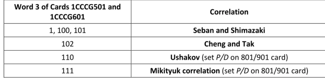
When a liquid metal (LBE or lead or sodium) is used as working fluid, a convective boundary condition must be set in the data for heat structures, in Word 3 of Cards 1CCCG501 and 1CCCG601, as reported in the following table (see Input Manual of RELAP5).
Table 2.1: Choice of Correlation in Word 3 of Cards 1CCCG501 and 1CCCG601 of RELAP5 code
Word 3 of Cards 1CCCG501 and
1CCCG601 Correlation
1, 100, 101 Seban and Shimazaki
102 Cheng and Tak
110 Ushakov (set P/D on 801/901 card)
3. Description of the NACIE loop facility
Since 1999 the ENEA Brasimone research center has been strongly involved in Heavy Liquid Metal (HLM) technology development, acquiring large competences and capabilities in the field of HLM thermal-hydraulic, coolant technology, material for high temperature applications, corrosion and material protection, heat transfer and removal, component development and testing, remote maintenance, procedure definition and coolant handling.
In this frame, the Natural Circulation Experiment (NACIE) has been set up to qualify and characterize components, system and procedures relevant for HLM nuclear technologies. In particular, NACIE facility sees several experiments performed in the field of thermal hydraulics and fluid dynamics in order to obtain heat transfer correlation in prototypical fuel bundle simulators. NACIE experimental campaign is essential for GEN IV nuclear power plant design and for the qualification and development of CFD code and Thermal-Hydraulics system code.
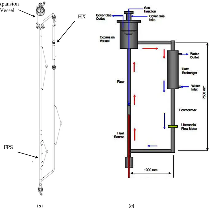
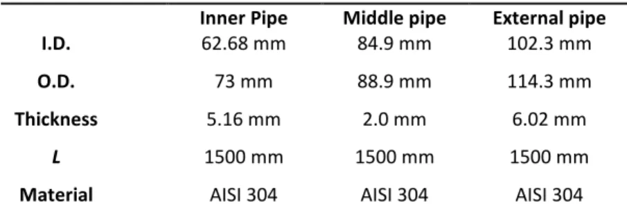
NACIE [6], [7] is a loop type facility filled with Lead-Bismuth Eutectic (LBE). It basically consists of a rectangular loop made of two vertical stainless steel (AISI 304) pipes (Nominal Pipe Size (NPS) 2½'' schedule 40) acting as riser and downcomer connected by means of two horizontal pipes of the same dimension. The heat source is installed in the bottom part of the riser, while the upper part of the downcomer is connected through appropriate flanges to a heat exchanger (see Figure 3.1). The overall height measured between the axis of the upper and lower horizontal pipes is 7.5 m and the width is 1 m. The total inventory of LBE is in the order of 1000 kg and the loop is designed to work with temperature and pressure of about 550°C and 10 bar respectively. The facility can work both in natural and forced circulation conditions; furthermore the transition from forced to natural circulation can be investigated. Regarding the operation under natural circulation regime, the thermal centers elevation (H ≈ 5.7 m) between the heat source (FPS) and the heat sink (Heat Exchanger, HX) provides the pressure head ∆p~gβ∆T⋅H required to guarantee a suitable LBE mass flow rate.
To promote the LBE mass flow rate along the loop under forced circulation condition, a gas lift technique was adopted. A pipe with an I.D. of 10 mm is housed inside the riser connected through the top flange of the expansion gas to the argon feeding circuit, while at the lower section of the pipe, a nozzle is installed to inject argon into the riser promoting enhanced circulation inside the loop. The Gas injection system is able to supply argon flow rate in the range 1-75 Nl/min with a maximum injection pressure of 5.5 bar. The argon gas flows into the riser and it is finally separated (in the expansion gas) from the double phase mixture, flowing upwards into the cover gas while the LBE flows into the heat exchanger through the upper horizontal branch. According to the described configuration, the
maximum LBE mass flow rate is around
5 kg/s in natural circulation and 20 kg/s in forced circulation condition.
The primary LBE side is coupled to the water secondary side by means of “tube in tube” counter flow type heat exchanger (HX) fed by water at low pressure (about 1.5 bar). It was designed assuming a thermal duty of 30 kW adopting tube-in-tube technology with LBE tube side, water shell side and steel powder filling the gap. The HX essentially consists of three coaxial tubes with different thicknesses (see
Table 3.1 and
Figure 3.2). LBE flows downward into the inner pipe of the HX, while water flows upwards in the annular region between the middle and the outer pipe allowing a counter current flow heat exchange. The annular region between the inner and middle pipes is filled with stainless steel powder. The aim of this powder gap is to ensure the thermal flux between LBE and water and to reduce the thermal stress across the tube walls (the thermal gradient between LBE and water is localized across the powder layer). Moreover the three pipes are welded together in the lower section while in the upper section, the inner pipe is mechanically decoupled from the other pipes allowing axial expansion between them.
In order to avoid a powder leakage, the annular region (filled by the powder) is closed in the upper section by a graphite stopper. In the outer pipe an expansion joint is installed to mitigate the stresses due to different axial expansion between the middle and the outer pipe walls.
(a) (b)
Figure 3.1: Isometric view (a) and layout (b) of the primary loop of the NACIE facility
HX
FPS Expansion
Figure 3.2: NACIE heat exchanger
Table 3.1: NACIE heat exchanger geometrical data Inner Pipe Middle pipe External pipe
I.D. 62.68 mm 84.9 mm 102.3 mm
O.D. 73 mm 88.9 mm 114.3 mm
Thickness 5.16 mm 2.0 mm 6.02 mm
L 1500 mm 1500 mm 1500 mm
Material AISI 304 AISI 304 AISI 304
The secondary circuit is then completed by a fan cooler to maintain water temperature under the boilingpoint (see Figure 3.3).
The NACIE bundle (see Figure 3.4) consists of two high thermal performance electrical pins with a nominal thermal power of about 43 kW; the main characteristics of the bundle are summarized in Table 3.2.
Figure 3.4: NACIE electrical fuel pin bundle
Table3.2: NACIE bundle main data N° of active pins 2
O.D. 8.2 mm
Total length 1400 mm Active length 850 mm
4. NACIE experimental campaign
The last experimental activity performed on the NACIE loop [8] included a series of 10 test concerning natural circulation, forced circulation and transition from forced to natural condition and vice-versa. Each test has been performed with only one pin activated in the heating section, with a maximum nominal power of 21.5 kW. In Table 4.1 the test matrix adopted for the experimental campaign is reported.
Table 4.1: Test matrix Name Tav [°C] Power % Power [kW] Ramp t
[min] Heat sink
G_lift [Nl/min] Transition NC to FC Transition FC to NC 201 200-250 50 9.5 5 YES 0 NO NO 203 200-250 50 9.5 5 YES 5 NO YES 204 200-250 50 9.5 5 YES 2,4,5,6,8, 10,6,5,4,2 YES NO 206 200-250 0 0 - NO 2,4,5,6,8, 10,6,5,4,3 NO NO 301 300-350 100 21.5 5 YES 0 NO NO 303 300-350 100 21.5 5 YES 5 NO YES 304 300-350 100 21.5 5 YES 2,4,5,6,8, 10,6,5,4,2 YES NO 305 300-350 50 9.5 5 YES 0 NO NO 306 300-350 0 0 - NO 2,4,5,6,8, 10,6,5,4,2 NO NO 406 350-360 25 3.5 5 NO 2,4,5,6,8, 10,6,5,4,2 NO NO
In Table 4.1, “Name” indicates the case name, Tav is the average reference temperature of LBE in the loop, “Power" is the power supplied to the Fuel Pin bundle Simulator (FPS), Ramp t is the time to reach the bundle power, “Heat Sink” is the activation of the secondary side (Yes= the secondary side and the HX are active as heat sink), G_lift is the gas-lift volumetric flow rate and the last to columns refers to the transition from Natural Circulation (NC) to Gas Lift Circulation (FC) or vice-versa during the specific test.
In the present work test 303 has been used to assess the NACIE RELAP5 model, according to the facility experimental setup previously described. The so obtained nodalization has then been used to perform coupled calculations (RELAP5/Fluent) based on the test 206 and test 306.
5 Thermal-hydraulic post-test analysis of NACIE
5.1 RELAP5 Model
The NACIE loop facility was modelled, on the basis of the configuration previously described, employing RELAP5/Mod3.3 [9] modified to implement LBE thermal fluid dynamics properties as reported in Section 2. Figure 5.1 depicts the adopted RELAP5 nodalization scheme: primary LBE loop and secondary water cooling circuit can be identified.
160 Expansion Vessel 1 1 1 2 0 125 1 3 0 146 148 Sep 150 156 152 170 1 7 2 1 8 0 5 1 0 TDV-500 (Water in)
HX
2 0 0 2 1.5 m 5.7 m 2.35 m 0.765 m 7.5 m TDJ-505 TDJ-405 TDV-520 (Water out) TDV-320 (Argon out) TDV-400 (Argon in) 5 mFPS
liquid metal follows an anticlockwise flow path through the loop components. LBE receives the supplied power flowing through Pipe-110 (FPS, Fuel Pin Simulator) placed in the bottom section of the Riser; FPS active length is characterized by a height of 0.89 m; a single electrical pin supplying heating power is simulated. Gas lift circulation has been modelled using TmdpJun-405 which connects TmdpVol-400 (containing argon) to Branch-125, injecting the required argon flow into the Riser (2.35 m from the bottom) and thereby promoting LBE circulation along the loop. Inside the Expansion Vessel argon is separated from the liquid metal and exits in TmdpVol-320; then, from the Expansion Vessel, LBE goes through the upper horizontal pipe (Pipe-160 and Pipe-170) to the downcomer where it flows downwards through the Heat Exchanger (HX) primary side section (Pipe-180, located on the downcomer upper zone). Here power is removed by the secondary side water flowing upwards, thermally coupled to the descending LBE. Secondary side water system is modelled by means of TmdpVol-500, (where the inlet water properties are set) connected to TmdpJun-505, that defines the inlet water mass flow rate feeding the HX secondary side annular zone (Annulus-510); water flows upwards and exits in TmdpVol-520. Primary to secondary heat transfer involves the 1.5 m HX active length and simulates the tube in tube counter flow heat exchanger configuration, taking into account the presence of stainless steel powder filling the gap created by the internal and middle pipe (5.95 mm width) described above (see Table 3.1 and Figure 3.2). Thermal conductivity of the powder has been chosen to be 10% of AISI 304 theoretical value. External heat losses have been considered as well. Taking into account the facility thermal insulation, a heat transfer coefficient with external environment, hext=1 W/m2K, has been imposed.
5.2 RELAP5 Post-Test Simulations
The experimental campaign carried out on NACIE loop consists of a series of 10 tests aiming at investigating the thermal hydraulic behaviour of the facility under natural circulation, forced circulation and the transition between the two regimes (see Table 4.1). The RELAP5 post-test simulations here analyzed focus on Test 303 designed to reproduce an Unprotected Loss of Flow (ULOF) like scenario. Table 5.1 summarizes the sequence of events characterizing the test.
Table 5.1: Test 303
Time
[h] Action Description
t0 0.0 Test starts LBE loop at rest. Initial temperature = 284°C t1 1.28 Argon on Activation of argon injection. Set flow = 5 Nl/min.
t2 1.78 FPS on Heat power supplied to fuel pin simulator. Mean power = 21.5 kW t3 1.86 HX on Activation of Heat Exchanger. Secondary water supply = 0.42 m
3 /h t4 5.85 Argon off ULOF event. Argon injection Shut off
t5 7.60 FPS and HX off Deactivation of heat power supply to FPS and feedwater to HX
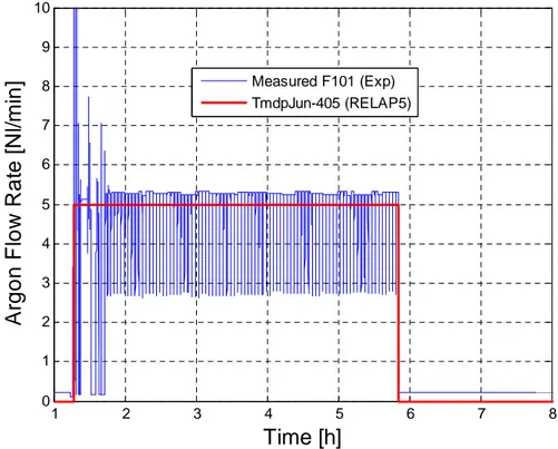
In the following, the time trends of boundary conditions set in RELAP5 input deck are compared with experimental data. Figure 5.2 shows the argon flow injected into the riser of NACIE to enhance LBE circulation. The experimental trends are measured by a gas flowmeter F101, while the value of 5 Nl/min has been adopted in RELAP5 simulation as reference for the gas mass flow rate provided by TmdpJun-405 for this test.
1 2 3 4 5 6 7 8 0 1 2 3 4 5 6 7 8 9 10
Time [h]
A
rg
o
n
F
lo
w
R
a
te
[
N
l/
m
in
]
Measured F101 (Exp) TmdpJun-405 (RELAP5)Figure 5.2: Argon flow rate time trend. Comparison of measured and value set by RELAP5 Electric power supplied during Test 303 to the pin simulator is plotted, as a function of time, in Figure 5.3 with heating power set in RELAP5 input deck. Electrical heating starts at t2=1.78 h, increasing linearly to the value of 21 kW in about 2 minutes. Afterwards the power profile shows a non constant trend especially in the first 2 hours from FPS activation. Power supply stops at t5=7.6 h.
5 10 15 20 25 30 35
P
o
w
e
r
[k
W
]
FPS R2 (Exp) FPS (RELAP5)has been taken to set RELAP5 boundary condition for the secondary water loop, that is, mass flow rate vs time (TmdpJun-505). HX is activated at t3=1.86 h and operates at t5=7.6 h. The two trends are plotted in Figure 5.4. Heat Exchanger feedwater is injected immediately after FPS activation and stops when FPS power is shut off. Inlet water mass flow rate is approximately equal to 0.12 kg/s.
1 2 3 4 5 6 7 8 0 0.05 0.1 0.15 0.2 0.25 0.3 0.35 0.4 0.45 0.5
Time [h]
W
a
te
r
F
lo
w
[
m
3/h
]
MP201 (Exp) TmdpJun-505 (RELAP5)Figure 5.4: Water Flow; comparison of measured and RELAP5 trends
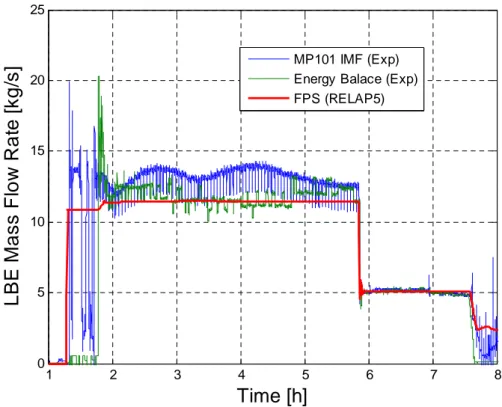
Figure 5.5 depicts LBE mass flow rate established during Test 303 in NACIE loop, both measured by the inductive flow meter MP101 and indirectly computed using the energy balance across the FPS. RELAP5 simulation results are compared to experimental data. LBE starts to circulate as argon injection starts (enhanced circulation); afterward, to simulate an ULOF accident, argon injection is deactivated (t4=5.85 h) and the flow is then solely driven by buoyancy phenomena (natural circulation). The vertical thermal centres (FPS and HX) distance is estimated to be 5.7 m. During the enhanced circulation regime, the measured mass flow rate reaches a mean value of about 13 kg/s characterized by oscillating behaviour mainly due to the argon injection compressor system, while heat balance evaluation gives a slightly lower value of about 12 kg/s, very close to the value estimated by the RELAP5 code. Afterward; in natural circulation regime, the mass flow rate drops to about 5 kg/s and good agreement can be observed between experimental data and RELAP5 results. After deactivation of FPS and HX at t5 the flow slowly decreases to zero.
1 2 3 4 5 6 7 8 0 5 10 15 20 25
Time [h]
L
B
E
M
a
s
s
F
lo
w
R
a
te
[
k
g
/s
]
MP101 IMF (Exp)Energy Balace (Exp) FPS (RELAP5)
Figure 5.5: LBE mass flow rate: comparison among measured, energy balance and RELAP5 trends LBE temperature profiles related to FPS inlet and outlet are plotted in Figure 5.6. Experimental values provided by thermocouples T109 (inlet) and T105 (outlet) are compared to RELAP5 results showing good agreement. RELAP5 initial LBE temperature has been set to 284°C for the whole loop assumed adiabatic till the FPS activation, to account for the external wire heaters employed in the experimental setup which maintain the required LBE temperature. Afterwards, a heat transfer coefficient towards the environment has been imposed setting the external air temperature and heat transfer coefficient, respectively equal to 20°C and 1 W/m2K. Following FPS and HX activation, temperatures start to increase up to a mean temperature of about 335°C (t=3.5 hours), then temperatures decrease reaching a near stationary condition (mean temperature of 320°C). It can be observed that the temperature profile reflects the power supply variation (see Figure 5.3); accuracy in reproducing FPS experimental power trend in RELAP5 model is mandatory to obtain adequate temperatures profile from the code. At this point ULOF event takes place deactivating gas injection (t4=5.85 h) and natural circulation establishes inside the loop. Inlet/outlet temperatures underwent a sudden decrease/increase of about 10°C followed by an ascending trend up to a new equilibrium value (after less than 2 hours) of 320°C and 348°C respectively, achieving a stationary state for this new regime. FPS and HX are then shut off (at t5=7.6 h) producing a rapid decrease of temperatures due to loop heat losses. RELAP5 outcome adequately reproduces the temperature profile characterizing the test and the transition from forced to natural regimes although slight discrepancies are observed mainly during ULOF transient phase. Experimental and RELAP5 inlet and outlet FPS temperature difference (from previous results) are plotted in Figure 5.7 showing good agreement. Figure 5.8 plots Heat Exchanger measured and simulated secondary water inlet and outlet temperatures. Experimental water inlet temperature, T201,
1 2 3 4 5 6 7 8 240 260 280 300 320 340 360
Time [h]
T
e
m
p
e
ra
tu
re
[
°C
]
FPS in T109 (Exp) FPS out T105 (Exp) FPS in (RELAP5) FPS out (RELAP5)Figure 5.6: Comparison between measured and calculated inlet and outlet FPS temperatures
1 2 3 4 5 6 7 8 0 5 10 15 20 25 30 35 40
Time [h]
T
e
m
p
e
ra
tu
re
D
if
fe
re
n
c
e
[
°C
]
FPS (Exp) FPS (RELAP5)1 2 3 4 5 6 7 8 0 20 40 60 80 100 120 140 160
Time [h]
W
a
te
r
T
e
m
p
e
ra
tu
re
[
°C
]
HX in T201 (Exp) HX out T202 (Exp) HX in (RELAP5) HX out (RELAP5)Figure 5.8: Comparison between measured and calculated inlet and outlet HX feedwater temperature
1 2 3 4 5 6 7 0 1000 2000 3000 4000 5000 6000
Time [h]
H
e
a
t
T
ra
n
s
fe
r
C
o
e
ff
ic
ie
n
t
[W
/(
m
2K
)]
FPS (RELAP5) HX1 (RELAP5) HX2 (RELAP5)profiles except for the LBE side bulk temperature which increases due to the lower heat transfer coefficient associated with the natural circulation regime. The powder gap (5.8 mm) represents the major contribute to the heat flux resistance with a temperature drop of about 180°C versus 25°C for the two walls (W1+W2), therefore, pointing out the importance in definig the thermal properties of the SS powder gap for the accuracy of model results.
31.4 36.5 42.4 44.4 50 100 150 200 250 300 350
Radius [mm]
T
e
m
p
e
ra
tu
re
[
°C
]
Asssisted t=5 h, (RELAP5) Natural t=7 h, (RELAP5)LBE
Water
W 1 GAP (powder) W2Figure 5.10: Temperature profile in HX double wall
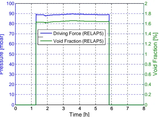
The available driving force, during the assisted circulation phase, has been evaluated from RELAP5 results as follows:
DF r
P
ρ
g H
∆
= ∆ ⋅ ⋅
(5.1)where Hr is the Riser height, set to 5.4 m, g gravity acceleration and ∆
ρ
is defined as:,
LBE r TP
ρ ρ
ρ
∆ = − (5.2)
and where
ρ
LBE andρ
r TP, are respectively LBE mean density and two phase flow mean density inside the Riser; these values are directly supplied by the code. The obtained driving force,∆
P
DF, for the assisted circulation phase, is plotted in Figure 5.11 together with the mean riser void fraction, showing respectively values around 90 mbar and 1.65%.0 1 2 3 4 5 6 7 8 0 10 20 30 40 50 60 70 80 90 100
Time [h]
P
re
s
s
u
re
[
m
b
a
r]
0 1 2 3 4 5 6 7 80 0.2 0.4 0.6 0.8 1 1.2 1.4 1.6 1.8 2V
o
id
F
ra
c
ti
o
n
[
%
]
Void Fraction (RELAP5) Driving Force (RELAP5)
6. RELAP5-Fluent coupled calculations
In this section, the in house coupling tool [10] and the preliminary obtained results are presented and compared with those obtained from stand-alone RELAP5 [9] and with the experimental data as well. The set up numerical model is based on a two-way semi-implicit coupling scheme. The vertical part of the loop including the heater system and part of the piping before and after it, has been simulated by the Fluent [11] code both in a simplified 2D axial-symmetric configuration and in a 3D configuration, while the remaining part of the loop has been simulated by the RELAP5 code.
6.1 RELAP5 and Fluent models
Starting from the previous NACIE RELAP5 nodalization (see Figure 5.1), NACIE primary circuit was re-arranged in such a way as to split the overall domain into two regions, one to be simulated by RELAP5 system code and one to be simulated using the Fluent CFD code (Non overlapping domains [12]). In particular the portion of the loop to be simulated by Fluent code is the Fuel Pin Simulator (FPS) of the loop (0.89 m see Figure 3.4) including a pipe of 0.21 m after it to reduce the possibility of occurrence of backflow conditions in the outlet section for the coupled code simulations, for an overall length of 1.1 m. In Figure 6.1 the RELAP5 nodalization used for the coupled simulations is reported. In TmdpJun-115 and in TmdpVol-112, respectively, boundary conditions of mass flow rate and temperature obtained from an inner reference section of the Fluent domain are applied; while the pressure imposed TmdpVol-110 is obtained from the inlet section of the CFD domain (see Figure 6.1). To reduce the occurrence of the previously mentioned backflow conditions in the outlet section of the CFD domain, a very high value of reverse form loss coefficient was set for the junction that connects Pipe-210 to Branch-100 and for the junction that connects Branch-125 with Pipe-130.
Concerning the part of the domain of Fluent competence, it was firstly simulated as a simplified 2D axial symmetric domain and then as a 3D symmetric domain in order to reduce the computational effort.
The 2D axial symmetric CFD domain was discretized by a structured mesh composed by 7668 rectangular cells, uniformly distributed both in the axial and radial coordinates (see Figure 6.2). The 3D symmetric domain was schematized with the symmetry plane passing through the axis of the electric pins (not reproduced in the model), the pin bundle retaining rods are not reproduced in the model as well (see Figure 6.3). The three-dimensional domain was then discretized using 141045 hexahedral elements with refinements near the inlet and outlet sections in axial direction and near the electric pins wall along the radial direction (see Figure 6.4).
To model the FPS form loss coefficient a constant value of 3.5 has been considered. For this purpose five different interior faces have been set as a porous-jump in the 2D domain and in each of them an equivalent constant coefficient of concentrate pressure drop value of 0.7 was set. The same value of the form loss coefficient has been inserted in the FPS of the RELAP5 nodalization used for stand-alone calculations. Regarding the 3D simulation one interior face has been set as porous-jumps and an equivalent constant coefficient of concentrate pressure drop equal to 0.5 was set in order to introduce the pressure drop due to the spacers grid not simulated in the 3D geometrical domain.
PIPE 100 0.05 m TDJ-115 160
Expansion
Vessel
125 1 3 0 146 148 Sep 150 156 152 170 1 7 2 1 8 0 5 1 0 TDV-500 (Water in)HX
2 0 0 2 0 6 1.5 m 1.05 m 0.765 m 7.5 m TDJ-505 TDJ-405 TDV-520 (Water out) TDV-320 (Argon out) TDV-400 (Argon in) 5 m TDV 112 TDV 110 Reference cell for pressure data neededfor Fluent outlet b.c.
Reference junction for flowrate data needed
for inlet Fluent b.c.
Reference section Reference section for flowrate and temperaure data needed for RELAP5 inlet b.c.
1.1 m
Figure 6.2: Axial-symmetric domain used in Fluent code for coupled simulations
Figure 6.3: 3D domain used in Fluent code for coupled simulations
Support rod
Electric Pins
Figure 6.4: Spatial discretization of the 3D domain
For the coupled simulations, uniform temperature and mass flux have been imposed at the inlet section of the geometrical domain for 2D and 3D simulations as well. In addition, for the same inlet section, a fixed turbulence intensity of 7% and the hydraulic diameter are imposed as boundary conditions for the turbulence equations. The turbulence model adopted in the CFD calculations is the RNG k-ε, while the thermo-dynamic properties of the LBE are considered as a function of temperature in agreement with the properties equation reported in Section 1.
6.2 Coupling procedure
The scheme applied to the coupling procedure between RELAP5 and Fluent codes is shown in Figure 6.5 [10]. The execution of the RELAP5 code is operated by an appropriate MATLAB script, where a processing algorithm is also implemented to receive boundary conditions (b.c.) data from Fluent, at the beginning of the RELAP5 time step, and to send b.c. data to Fluent code, at the end of the RELAP5 time step. In addition, a special User Defined Function (UDF) was realized for Fluent code to receive b.c. data from RELAP5 and to send b.c. data to RELAP5 for each CFD time step.
An initial RELAP5 transient of 1000 s has been executed to reach steady state conditions with a uniform temperature of 237°C for Test 206 and 285°C for Test 306 respectively and with fluid at rest. The end of this initial transient was considered time zero from which the coupled simulation started. After that, a sequential explicit coupling calculation is activated, where the Fluent code (master code) advances firstly by one time step and then the RELAP5 code (slave code) advances for the same time step period, using data received from the master code.
EXECUTE 1 TIME STEP OF FLUENT TRANSIENT CALCULATIONS
END OF THE FLUENT TIME STEP
WRITE FLUENT RESULTS NEEDED AS B.C. FOR RELAP5
EXECUTE RELAP5 TRANSIENT CALCULATIONS FOR 1 TIME STEP
TO RELAP
END OF TRANSIENT ?
WRITE RELAP5 RESULTS NEEDED AS B.C. FOR FLUENT
END OF RUN
Yes
No
Figure 6.5: RELAP5-Fluent coupling procedure
6.3 Matrix of simulations
The performed simulations are representative of a gas enhanced circulation test. The experiment chosen as a reference test for numerical simulation are Test 206 and Test 306 reported in the previous Table 4.1. A total of five simulations have been performed, three for Test 206 and two for Test 306. In particular a RELAP5 stand alone simulation, a coupled simulation using a Fluent 2D axis symmetric domain and a coupled simulation using a Fluent 3D symmetric domain have been carried out for Test 206 while for Test 306 a RELAP5 stand alone simulation and a coupled simulation using a Fluent 2D axis symmetric domain for Test 306 were performed. The argon mass flow rate injected in the riser is increased linearly in the first 5 seconds of the transient for each step and then maintained constant according to the experimental time table. A preliminary sensitivity analysis showed that the time step needed to guaranty the convergence and independency of the results from the adopted time step itself is in the order of 0.005 s. Transient simulations with fixed time step have been carried out for an overall simulated transient of 27000 s.
The test matrix of the performed simulations is shown in Table 6.1 reporting adopted boundary conditions and main monitored variables.
Table 6.1: Matrix of performed simulations
Name Tav [°C] FPS Power % Glift [Nl/min] Monitored variables
Test 206 200-250 0 2,4,5,6,8,
10,6,5,4,3
LBE flow rate Pin and Pout in the HS
Test 306 300-350 0 2,4,5,6,8,
10,6,5,4,3
6.4 Obtained results: Test 206 and Test 306
The LBE mass flow rate time trends obtained for Test 206 is reported in Figure 6.6, where the experimental results are compared with the calculated results both for the stand alone RELAP5 simulation and for the coupled RELAP5-Fluent 2D and 3D simulations.
0 1 2 3 4 5 6 7 8 0 2 4 6 8 10 12 14 16 18 20
L
B
E
M
a
s
s
F
lo
w
r
a
te
Time [h]
Experimental RELAP5 RELAP5+FLUENT 2D RELAP5+FLUENT 3DFigure 6.6: LBE mass flow rate results for Test 206
With respect to the experimental results, the calculated LBE mass flow rate overestimates them by less than 12%. Good agreement was found between the coupled code simulations with a 2D and 3D CFD domain, while the results of the coupled code simulations overestimate results obtained from the stand-alone RELAP5 by less than 5%.
0 1 2 3 4 5 6 7 8 1.12 1.13 1.14 1.15 1.16 1.17
D
if
fe
re
n
ti
a
l
P
re
s
s
u
re
[
P
a
]
Time [h]
RELAP5 RELAP5+FLUENT 2D RELAP5+FLUENT 3DFigure 6.7: FPS pressure difference for Test 206
Figure 6.8 shows the pressure time trend at the inlet and outlet sections of the FPS. The calculated pressure by the coupled codes and by RELAP5 code on the FPS inlet and outlet sections, are practically the same as those evaluated by the stand-alone RELAP5 code with differences lower than 0.5%.
0 1 2 3 4 5 6 7 8 7.8 8 8.2 8.4 8.6 8.8 9 9.2x 10 5
P
re
s
s
u
re
[
P
a
]
Time [h]
Inlet RELAP5 Inlet RELAP5+FLUENT 2D Inlet RELAP5+FLUENT 3D Outlet RELAP5 Outlet RELAP5+FLUENT 2D Outlet RELAP5+FLUENT 3DIn the following picture main results obtained from the coupled simulation with a 3D CFD geometrical domain are presented. In particular Figure 6.9 shows the pathlines colored by velocity along the vertical axis for t = 3.5 h (argon flow rate 10 Nl/min), the picture refers to a plane section placed a z = 0.89 m in correspondence with the end of the loop bundle.
Figure 6.9: 3D CFD domain: pathlines at the exit of the pin bundle, Test 206
Figure 6.10 shows the vector velocity (w, along z-direction). The magnitude of w (area-weighted z velocity) predicted by the CFD code at the outlet section of the 3D geometrical domain is about 0.88 m/s (t = 3.5 h argon flow rate 10 Nl/min).
of the supporting rod and vertical to the symmetry plane.
Figure 6.11: Distribution of turbulent kinetic energy k [m2/s2], Test 206
Figure 6.12 shows the LBE mass flow rate for Test 306. A good agreement is found between experimental results, those obtained from the stand-alone RELAP5 calculation and those obtained from the coupled simulation with 2D CFD domain. Maximum discrepancy between experimental and calculated results is less than 10%.
0 1 2 3 4 5 6 7 8 0 2 4 6 8 10 12 14 16 18 20
L
B
E
M
a
s
s
F
lo
w
r
a
te
Time [h]
Experimental RELAP5 RELAP5+FLUENT 2DFigure 6.12: LBE mass flow rate results for Test 306
Figure 6.13 shows the pressure difference between the inlet and outlet section of the FPS. As it can be noted, the pressure drop in the FPS calculated by the Fluent code in the 2D coupled simulation fits well
with results obtained from stand-alone RELAP5 simulation showing a difference between them that is lower than 1%. 0 1 2 3 4 5 6 7 8 1.11 1.12 1.13 1.14 1.15 1.16 1.17 1.18 x 10⁵ D if fe re n ti a l P re s s u re [ P a ] Time [h] RELAP5 RELAP5+FLUENT 2D
Figure 6.13: FPS pressure difference for Test 306
Figure 6.14 shows the pressure time trend at the inlet and outlet sections of the FPS for Test 306. The pressure calculated by the coupled codes on the FPS inlet and outlet section, are practically the same as those evaluated by the stand-alone RELAP5 code as observed for Test 206 with differences between them lower than 0.5%.
8 8.2 8.4 8.6 8.8 9 9.2x 10 5 P re s s u re [ P a ] Inlet RELAP5 Inlet RELAP5+FLUENT 2D Outlet RELAP5 Outlet RELAP5+FLUENT 2D
0 2 4 6 8 10 12 14 16 0 2 4 6 8 10 12 14 16
Experimental LBE Flow Rate [kg/s]
C a lc u la te d L B E F lo w R a te [ k g /s ] RELAP5 (TEST 206) RELAP5 (TEST 306) RELAP5+FLUENT 2D (TEST 206) RELAP5+FLUENT 2D (TEST 306) RELAP5+FLUENT 3D (TEST 206)
7 Thermal-hydraulic post-test analysis of ICE-DHR
In order to assess the RELAP5 prediction capability for LBE pool type system, a post-test simulation was performed on CIRCE experimental campaign housing the upgraded ICE test section with a decay heat removal system (DHR). The reference experiment, Test IV, reproduces an accidental event characterized by a total loss of secondary circuit followed by reactor scram and DHR activation to remove the residual heat generation. The test is representative of a protected loss of heat sink scenario combined with primary circuit loss of flow (PLOH+LOF). The thermal hydraulic behavior of the system and the transition from forced to natural circulation were investigated.
7.1 Post-Test RELAP5 simulations
RELAP5 code [9] modified/implemented as described in Section 5 for NACIE simulation, was used to analyze the above described Test IV. The nodalization scheme adopted for CIRCE experiments simulations is depicted in Figure 7.1.
0.26 m above the Riser outlet. The LBE enters into the aspiration duct from the pool bottom, reaching the Fuel Pin Simulator bundle (FPS), where it is heated (1 m active length, Pipe-60); it then flows upstream, crossing the fitting volume (Pipe-90), through the Riser (Pipe-130) and reaches the separator located in the upper part of the facility. A time dependent junction (TmdpJun-4) is connected to the Riser inlet (Branch-100) and injects argon (from Tmdpvol-4) to simulate the gas lift system during the assisted circulation phase. In the Separator (Branch-132), the gas is separated from the liquid metal and goes up in the vessel cover gas plenum (Branch-150), while the hot LBE goes downwards through the main Heat Exchanger (HX) shell (Pipe-170), to be cooled by the HX secondary water. The LBE exits flowing through a flow straightener (Pipe-172), placed in the lower part of the shell, into the downcomer. The pool external zone (Pipe/Branch from 200 to 260) was modeled by means of a series of parallel pipes connected by branches; such a nodalization of the pool, aims at improving the simulation of LBE mixing and thermal stratification phenomena observed experimentally.
The DHR primary side consists in an annular channel region modeled by Pipe-180. During the DHR activation, the hot LBE flows downwards from the pool top region (Branch-138) through the DHR primary side annular channel (Pipe-180). Here, LBE is cooled by the secondary side air flowing upstream through the DHR internal pipe, in a counter current heat exchanger configuration. The LBE cooled by the DHR exits in the pool through the DHR skirt (Pipe-182). Heat generation inside the FPS is simulated by an average heat structure representing the 37 electrical pins; the convective boundary condition is set according to Ushakov correlation [14] for rod bundle. Similarly, the same correlation is used for the HX primary side convective heat transfer with the 91 tubes. Heat transfer of LBE from the main flow-path to the quasi-stagnant LBE inside the pool was considered as well, with the exception of the Riser and the DHR shell which are thermally insulated, therefore considered adiabatic in the simulations. Heat dispersion of the LBE inside the tank towards the containment building was taken into account introducing an air convective heat transfer coefficient around hext =1.5 W/(m
2
K). Pressure losses along the main flow path were taken into account introducing concentrated pressure losses coefficients to simulate the presence of the Venturi nozzle (placed to measure the LBE flow) and the spacer grids.
The HX secondary side is modeled by three water loops, simulating the three compartments of 7 (inner), 54 (middle) and 30 (outer) bayonet tubes in which the HX bundle is arranged. Water is injected (Tmdpjun-801) inside each loop through three Motor Valves, flows downwards into the inner pipe and rises up through the annular region, where it exchanges heat in counter current with the primary LBE. Along the annular zone length, water begins to change its phase and the water/steam mixture is finally collected in the Steam Plenum (Pipe-700). The secondary side is thermally coupled with the primary side by means of an adequate heat structure between the water/steam mixture inside the annular zone and the LBE flowing through the tube bundles; a cylindrical double wall with helium inside the gap was modeled to compute the heat conduction. Vertical bundle without crossflow (with a p/d=1.32) convective condition type is set for the right boundary condition (LBE side), whereas the default convection condition is set for left boundary conditions (water/steam). A heat structure is foreseen to take into account the heat transfer between the cold water flowing in the inner tube and the water/steam mixture flowing through the annular zone. The bayonet tube of the DHR secondary side system is simulated according to design parameters. The air mass flow rate is imposed at the inner tube inlet section by means of a time dependent junction (Tmdpjun-310); air goes down towards the tube bottom plate and then flows upwards through the annular region up to the air Plenum located above the tank S100 cover. As for the HX, a heat structure provides the thermal coupling of the
primary and secondary fluids of the DHR system. Heat transferred between inner tube and annular region, is taken into account as well.
7.2 Test IV. Initial and Boundary Conditions
Test IV starts with CIRCE facility maintained at isothermal conditions (320°C) by means of heaters which compensate heat losses. In Figure 7.2 boundary conditions used for Test IV are illustrated.
30 0 7 48 Time [h] FPS Power 0.225 Kg/s 0.65 kg/s 693.5 kW 47.5 kW
Air Injection (Ti=20 °C )
PLOH + LOF Transient
H2O Injection (Ti=10 °C ) Argon Injection
1.78 Nl/s
Figure 7.2: Boundary condition for Test IV
The RELAP5 simulation post-test analysis reproduces the experimental actions sequence performed during Test IV; the main boundary condition (FPS power, argon flow, and secondary fluid mass flow rates) are taken from the experimental outcomes. Namely, the simulation begins with the injection of argon (approximately 1.78 Nl/s) inside the Riser to enhance primary LBE circulation. After reaching a stabilized value of the primary flow, power is supplied (power ramp) to the FPS up to a nominal value of 693.5 kW. Simultaneously, the main Heat Exchanger is activated by injecting 0.65 kg/s of water inside the 91 bayonet tubes in order to remove the supplied thermal power. This condition is maintained for several hours in order to attain a well stabilized condition in the primary system before beginning the transient phase. After about 7 hours from the beginning, the PLOHS+LOF transient is initialized performing the following procedures:

![Table 4.1: Test matrix Name T av [°C] Power % Power [kW] Ramp t](https://thumb-eu.123doks.com/thumbv2/123dokorg/5628300.68852/20.892.95.810.322.690/table-test-matrix-t-av-power-power-ramp.webp)