Luca Giuzzi
Hermitian varieties over finite fields
Thesis submitted for the award of the degree of Doctor of Philosophy
This research work has been funded by an INDAM scholarship of the Italian ‘Istituto Nazionale di Alta Matematica’ and by a bursary of the Engineering and Physical Sciences Re-search Council, which covered tuition fees. I am most grateful to these organisations for their support.
Among the several people which have helped me during the work on this thesis I would like to explicitly thank my supervisor, Prof. J.W.P. Hirschfeld, both for his constant advice on the research and for having taught me how to write scientific prose. I would like to thank also Professors G. Korchm´aros and A. Cossidente from Potenza for very helpful discussions on the topics investigated here.
I would like to express once more my gratitude towards my parents for their continuous support and understanding.
Finally, I wish to thank in a special way Jennifer Huynh for her kindness and our excellent friendship, and all the other people that, in one way or another, have been near me during all these years.
more new experiments left for the tryal of other men that succeed us.
In this work, submitted for the award of the title of Doctor of Philosophy, we have investigated some properties of the configurations arising from the intersection of Hermitian varieties in a finite projective space.
Chapter 1 introduces some background material on the theory of finite fields, projective spaces, Hermitian varieties and classical groups.
Chapter 2 deals with the 2-dimensional case. In Section 2.1, we present the the point-line classification of the intersections, due to Kestenband. In Section 2.2, we determine the full linear collineation group stabilising any of the configurations of 2.1 and we prove that if two configurations have the same point-line structure, then they are in fact projectively equivalent. A new and simplified proof of the group theoretical characterization of the Hermitian curve as the unital stabilised by a Singer subgroup of order q −√q + 1 closes the chapter in Section 2.3.
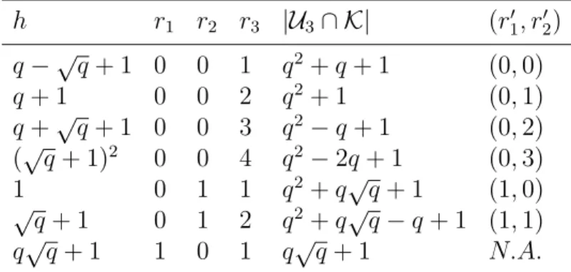
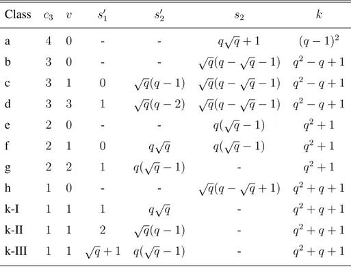
In Chapter 3 we study the 3-dimensional case. In Section 3.1 we determine what incidence configurations fulfill the combinatorial properties required in order to be the intersection of Hermitian surfaces. Section 3.2 presents some further general remarks on linear systems of Hermitian curves and extensive computations on 4 × 4 Hermitian matrices. In Section 3.3, we produce models that realize all the possible intersection configurations in dimension 3.
Chapter 4 is organized in two independent sections. In Section 4.1 we provide a general formula to determine the list of possible sizes of Hermitian intersections in PG(n, q). The for-mula itself has been obtained by studying the geometry of the set H of all singular Hermitian hypersurfaces of PG(n, q). Such a set is endowed with the structure of an algebraic hypersur-face of PG(n2 + 2n, q) of degree n + 1; the locus of the singular points of H is analyzed
in detail. In Section 4.2 we introduce some computer code in order to explicitly compute the intersection configurations arising in PG(n, q).
Introduction 1
1 Preliminary results 3
1.1 Permutation Groups . . . 3
1.1.1 Definitions . . . 3
1.1.2 Transitivity and regularity . . . 3
1.1.3 Similarities . . . 4
1.1.4 Actions and representations . . . 5
1.2 Finite fields . . . 5
1.2.1 Definitions and models . . . 5
1.2.2 Automorphisms and extensions . . . 7
1.2.3 Trace and norm . . . 8
1.3 Projective spaces . . . 10
1.3.1 Incidence structures . . . 10
1.3.2 Algebraic constructions . . . 13
1.3.3 Morphisms . . . 15
1.3.4 Singer cyclic groups . . . 16
1.4 Polynomials and matrices . . . 17
1.4.1 Definitions . . . 17
1.5 Varieties over finite fields . . . 18
1.5.1 Polynomials as functions over projective spaces . . . 18
1.5.2 Algebraic sets and ideals . . . 19
1.5.3 Number of rational points: zeta functions . . . 20
1.5.4 Dimension . . . 21
1.5.5 Non-singular varieties . . . 22
1.6 Unitary Groups . . . 22
1.6.1 Definitions . . . 23
1.6.2 Subspaces and forms . . . 25
1.6.3 Hermitian groups . . . 25
1.6.5 Morphisms and automorphisms . . . 26
1.7 Hermitian Forms and Hermitian varieties . . . 27
1.7.1 Hermitian matrices . . . 27
1.7.2 Hermitian forms . . . 28
1.7.3 Hermitian hypersurfaces: definitions . . . 30
1.7.4 Hermitian sub-varieties and points . . . 32
1.7.5 Hermitian varieties and unitary groups . . . 33
1.7.6 Polarities . . . 34
1.7.7 Subspaces in Hermitian varieties . . . 36
1.7.8 Incidence properties . . . 36
2 The 2-dimensional case: Hermitian curves 37 2.1 Classification of intersections in dimension 2 . . . 37
2.1.1 Incidence classification . . . 37
2.1.2 Outline of the proof . . . 40
2.2 Groups of the intersection of two Hermitian curves . . . 42
2.2.1 Introduction . . . 42
2.2.2 A non-canonical model of PG(2, q) . . . . 43
2.2.3 Equations for the non-singular Hermitian curve . . . 44
2.2.4 Groups preserving the intersection of two Hermitian curves . . . 45
Class I . . . 46 Class II . . . 48 Class III . . . 51 Class IV . . . 53 Class V . . . 56 Class VI . . . 56 Class VII . . . 57
2.3 A group-theoretic characterization of Hermitian curves as classical unitals . . . 58
2.3.1 Introduction . . . 58
2.3.2 A result on classical unitals . . . 58
2.3.3 Proof of Theorem 2.3.1 . . . 59
3 The 3-dimensional case: Hermitian surfaces 61 3.1 Description of incidence configurations in dimension 3 . . . 61
3.1.1 Some general remarks on cones . . . 63
3.1.2 Pencils whose degenerate surfaces have all rank 3 . . . 65
3.1.3 Pencils whose degenerate surfaces have all rank 2 . . . 68
3.1.4 Pencils whose degenerate surfaces have ranks 2 and 3 . . . 71
3.2 Hermitian matrices and polynomials . . . 73
3.2.1 Some general considerations on Hermitian pencils . . . 78
Further linear algebra observations . . . 79
3.2.2 Case I: 3 or 4 distinct roots . . . 81
3.2.3 Case II: 2 distinct roots . . . 82
3.2.4 Case III: 1 root . . . 84
3.2.5 Case IV: some notes when the factorisation contains irreducibles . . . . 87
3.3 Construction of the incidence configurations . . . 90
3.3.1 Pencils with degenerate surfaces of rank 3 only . . . 90
3.3.2 Pencils with degenerate surfaces of rank 2 only . . . 92
3.3.3 Pencils whose degenerate surfaces have rank 2 and 3 . . . 93
4 General results 97 4.1 The cardinality formula . . . 97
4.1.1 Introduction . . . 97
4.1.2 Preliminaries . . . 97
4.1.3 The determinantal variety H . . . 101
4.1.4 Action of PGL(n + 1, q) on H . . . 106
4.1.5 The order formula . . . 108
4.1.6 Some further remarks on H . . . 110
4.2 Explicit computations and algorithms . . . 112
4.2.1 The computer code: general remarks . . . 112
4.2.2 Initialization: main and param . . . 113
4.2.3 Auxiliary functions: Projective and Helpers . . . 114
4.2.4 Preliminary computations: Prelim.gap . . . 125
4.2.5 Unitary group construction: Unitary.gap . . . 129
4.2.6 Orbit computation: Orbits.gap . . . 131
4.2.7 Intersection and results output: Post-orb.gap . . . 132
4.2.8 Generators of the projective unitary group . . . 138
Quasi-symmetries . . . 138
Ishibashi’s theorem . . . 140
4.2.9 Concluding remarks . . . 143
1.1 Veblen-Young configuration . . . 12
1.2 Desargues configuration . . . 13
1.3 Pappus configuration . . . 14
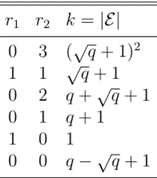
2.1 Possible intersection numbers for non-degenerate Hermitian Curves. . . 38 2.2 Minimal polynomials corresponding to given rank sequences in the 2-dimensional
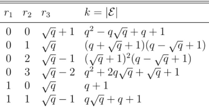
case. . . 40 2.3 Canonical forms for 3 by 3 Hermitian matrices. . . 40 2.4 Equations for the non-degenerate Hermitian curve . . . 44 3.1 Possible intersection numbers for Hermitian surfaces: non-degenerate pencil. . 62 3.2 Possible intersection numbers for Hermitian surfaces: degenerate pencil; r3 6=
0, r4 = 0. . . 62
3.3 Possible intersection numbers for Hermitian surfaces: degenerate pencil; r2 6=
0, r3 = r4 = 0. . . 62
3.4 Possible intersections E between a cone and a non degenerate Hermitian sur-face; vertex not in the intersection. . . 64 3.5 Indices for the intersection of a cone and a Hermitian surface. . . 65 3.6 Possible incidence classes for two non-degenerate Hermitian surfaces: Γ
con-tains degenerate surfaces of rank 3 only. . . 68 3.7 Possible incidence classes for two non-degenerate Hermitian surfaces: Γ
con-tains degenerate surfaces of rank 2 only. . . 70 3.8 Indices for the intersection of Hermitian surfaces of rank 2 and of rank 3. . . . 71 3.9 Possible incidence classes for two non-degenerate Hermitian surfaces: Γ
con-tains degenerate surfaces of ranks 2 and 3. . . 74 3.10 Canonical forms for the 3-dimensional case: MH(x) splits over GF(√q); 2 or
3 distinct roots. . . 75 3.11 Canonical forms for the 3-dimensional case: MH(x) splits over GF(√q); 1 or
4 roots. . . 76 3.12 Canonical forms for the 3-dimensional case: MH(x) does not split over GF(√q);
degree 4. . . 77 4.1 Intersection numbers for non-degenerate Hermitian varieties in dimension 4. . . 110 4.2 Dimension of the varieties O≥t for small n . . . 111
A projective space PG(n, q) admits at most three types of polarity: orthogonal, symplectic and unitary. The absolute points of an orthogonal polarity constitute a non-degenerate quadric in PG(n, q); for a symplectic polarity, all the points of PG(n, 2t) are absolute; the locus of all
absolute points of a unitary polarity is a non-degenerate Hermitian variety.
Non-degenerate Hermitian varieties are unique in PG(n, q) up to projectivities. However, two distinct Hermitian varieties might intersect in many different configurations. Our aim in this thesis is to study such configurations in some detail.
In Chapter 1 we introduce some background material on finite fields, projective spaces, collineation groups and Hermitian varieties.
Chapter 2 deals with the two-dimensional case. Kestenband has proven that two Hermitian curves may meet in any of seven point-line configurations. In Section 2.1, we present this classification. In Section 2.2, we verify that any two configurations belonging to the same class are, in fact, projectively equivalent and we determine the linear collineation group stabilizing each of them. Such a group is usually quite large and is transitive on almost all the points of the intersection. A subset U of PG(2, q) such that any line of the plane meets U in either 1 or
√
q + 1 points is called a unital. A Hermitian curve is a classical unital. However, there exist
non-classical unitals as well. In Section 2.3 we present a short proof of a characterisation of the Hermitian curve as the unital stabilized by a Singer subgroup of order q −√q + 1.
In Chapter 3, we describe the point-line-plane configurations arising in dimension 3 from intersecting two Hermitian surfaces. Our approach consists first in determining some combi-natorial properties the configurations have to satisfy and then in actually constructing all the possible cases. Section 3.1 presents the list of all possible intersection classes; after some more technical results in Section 3.2, in Section 3.3 we construct linear systems of Hermitian sur-faces yielding the wanted configurations for any class. In this chapter we deal with intersections which contain at least√q + 1 points on a line.
Chapter 4 is divided into two independent sections: in Section 4.1 we study the determinan-tal variety of all the (n+1) ×(n+1) Hermitian matrices as a hypersurface of PG(n2+2n,√q).
From the study of such a variety we are able to determine the list of all possible intersection sizes for any dimension n. In Section 4.2 we present some computer code in order to produce pencils of Hermitian varieties in PG(n, q). This code, however, is able to provide useful
re-Preliminary results
The aim of this first chapter is to recall some known results that will be used throughout the thesis.
1.1 Permutation Groups
Our main reference for the theory of finite permutation groups is [Wie64]. For general results on group theory, [Rob80] has been used.
1.1.1 Definitions
Definition 1.1.1. Let X be a non-empty set. A permutation of X is a bijective mapping of X into itself. The set of all permutations of X, together with map composition forms a group SX,
the symmetric group on X.
Definition 1.1.2. A permutation group G on a set X, or an X-permutation group, is any sub-group of SX. The degree of a permutation group G is the cardinality of the set X it acts upon.
Definition 1.1.3. Let G be an X-permutation group and define † as the equivalence relation on
X given by
x † y ⇐⇒ ∃σ ∈ G : x = σ(y).
The equivalence classes of † are the orbits of G on X. The orbit of any x ∈ X will be denoted by the symbol xG.
1.1.2 Transitivity and regularity
Definition 1.1.4. A permutation group G is transitive on X if and only if it has only one orbit, namely X itself.
Definition 1.1.5. For any X-permutation group G and for any Y ⊆ X, the stabilizer of Y in G is the set
StG(Y ) := {σ ∈ G : ∀y ∈ Y : σ(y) ∈ Y }.
A group G is semi-regular if for any x ∈ X, StG(x) = 1; G is regular if it is semi-regular and
transitive.
Definition 1.1.6. Let n be a positive integer. A permutation group G is 1-transitive on X if and only if it is transitive on X. A group G is n-transitive on a set X if and only if for any x ∈ X,
StG(x) is (n − 1)-transitive on X \ {x}.
Lemma 1.1.7. Assume that G is a n-transitive group on X. Then, (i) for any x ∈ X, StG(x) is (n − 1)-transitive on X \ {x};
(ii) given two tuples lx = (x1, . . . , xn), ly = (y1, . . . , yn) of elements of X, there exists a
permutation σ ∈ G such that σ(lx) = ly.
Definition 1.1.8. A group G is strictly n-transitive on X if it is n-transitive and, given any two different n-tuples lx, ly of distinct elements of X, there exists exactly one σ ∈ G such that
σ(lx) = ly.
Lemma 1.1.9. Let G be a permutation group on a set X. Then, for any x ∈ X,
|G| = |xG||St G(x)|.
1.1.3 Similarities
Definition 1.1.10. Let G be an X-permutation group and H be a Y -permutation group. A
similarity between G and H is a pair (α, β), where
(i) α is an isomorphism between G and H; (ii) β is a bijection between X and Y ; (iii) for any σ in G and for any x ∈ X,
β(xσ) = (β(x))α(σ).
Two permutation groups are similar if there is a similarity between them.
The sets X and Y have to be isomorphic in order for G and H to be similar; still, |X| = |Y | and G ' H is not sufficient for G and H to be similar.
1.1.4 Actions and representations
Definition 1.1.11. Let G be a group and let X be a non-empty set. A right action of G on X is a function ρ : X × G → X such that
ρ(x, g1g2) = ρ(ρ(x, g1), g2).
In an analogous way, a left action of G on X is defined as a function λ : G × X → X such that
λ(g1g2, x) = λ(g1, λ(g2, x)).
Definition 1.1.12. Let G be any group and let X be a set. Any group homomorphism γ :
G → SX is a permutation representation of G on X and it induces a right action on X via the
mapping (x, g) → γ(g)x.
The cardinality of X is the degree of the representation γ. If ker γ = {1}, then the repre-sentation is faithful; a reprerepre-sentation is transitive if its image in SX is transitive; γ is regular if
its image in SX acts regularly on X.
1.2 Finite fields
The reference text for most of the definitions and results presented in this section is [LN97].
1.2.1 Definitions and models
Definition 1.2.1. A ring (R, +, ·) is an integral domain if, for all x, y ∈ R, xy = 0 implies
x = 0 or y = 0; if (R \ {0}, ·) is a group, then the ring R is a division ring. A division ring R
in which the group R? = (R \ {0}, ·) is Abelian is a field; a division ring in which the group R?
is non-commutative is a skew-field.
Theorem 1.2.2 (Wedderburn, 1905). Every finite division ring is a field.
Definition 1.2.3. The characteristic of a ring (R, +, ·) is the smallest positive integer char(R) =
n such that for all r ∈ R:
nr := r + . . . + r| {z } n times
= 0. If no such an n exists, R is said to have characteristic 0.
Definition 1.2.4. A subfield K of a field (F, +, ·) is a subset of F which is closed under the field operations. The field (F, +, ·) is called an extension (field) of (K, + |K, · |K). The symbol
K ≤ F is used to denote that F is an extension field of K or, equivalently, that K is a subfield
Any field contains itself, the empty set and the set consisting of its zero only as subfields. Those subfields are called trivial.
Definition 1.2.5. A field is prime if it does not contain any proper subfield. Lemma 1.2.6. Any subfield has the same characteristic as its parent field.
Definition 1.2.7. Let K be a subfield of F and assume f ∈ F . The extension of K by f is the smallest subfield K(f ) of F such that,
K ∪ {f } ⊆ K(f ) ⊆ F.
Definition 1.2.8. Given a field K, its algebraic closure K is the smallest field containing K such that any polynomial
n
X
i=0
kixi ∈ K[x]
splits to linear factors in K[x].
Lemma 1.2.9. Let Z be the ring of integers, p a prime number and let pZ be the ideal generated
by p in Z; then, Z/(pZ) is a finite field containing p elements.
Proof. Let Fp := {0, . . . , p − 1} ⊂ Z, and let φ be the projection mapping
φ :
½
Fp → Z/(pZ)
x → x + (pZ).
Define, for any b, c ∈ F ,
b + c := φ−1(φ(b + c)); b · c := φ−1(φ(bc)).
The structure (Fp, +, ·) is closed under its operations and every non-zero element admits an
inverse. It follows that F is a field.
Definition 1.2.10. The field (Fp, +, ·) constructed in the previous lemma is called the Galois
field with p elements. It will be denoted by the symbol
GF(p) := (Fp, +, ·).
Definition 1.2.11. Let (F, +, ·) and (G, ⊕, ¯) be two fields. A morphism between F and G is a mapping φ : F → G preserving the algebraic structure; that is, for all p, q ∈ F :
(i) φ(p−1) = φ(p)−1,
(iii) φ(pq) = φ(p) ¯ φ(q), (iv) φ(p + q) = φ(p) ⊕ φ(q).
A necessary condition for a morphism to exist between two fields F and G is that char(F ) = char(G).
Monomorphisms, epimorphisms, isomorphisms and automorphisms are defined the usual way.
Theorem 1.2.12. Any field K contains a prime subfield F which is either isomorphic to the
field of the rational numbers Q or to GF(p) for some prime p, according as the characteristic of K is 0 or p.
Theorem 1.2.13. Let F be a finite field. Then, the cardinality of F is pn, where p = char(F ) is
a prime number and n is an integer. The integer n is called the degree of F over its prime field.
As a matter of fact, the converse is true as well.
Theorem 1.2.14. For every prime p and for every integer n there exists a finite field F of order
pn. All fields of given order q = pn are isomorphic to the splitting field of the polynomial
(xq− x) over GF(p). This field F will be written as
GF(q) := GF(p)[x]/(xq− x).
Definition 1.2.15. Given any finite field (F, +, ·), its multiplicative group F?is cyclic. A
gen-erator of F? is a primitive element of F .
1.2.2 Automorphisms and extensions
Lemma 1.2.16. Let F be a finite extension field of GF(q). Then, there exists an integer m > 0
such that F = GF(qm). This integer is the degree of F over GF(q) and is written as
[F : GF(q)] := m.
Definition 1.2.17. Let GF(qm) be an extension field of GF(q), and let α ∈ GF(qm). The
elements α, αq, . . . , αqm−1
are called the conjugates of α with respect to GF(q).
Definition 1.2.18. An automorphism of GF(qm) over GF(q) is a field automorphism of GF(qm)
which fixes all the elements of GF(q). The group of all these automorphisms is the Galois group of GF(qm) over GF(q) and it is denoted by the symbol
Gal(GF(qm) : GF(q)).
Lemma 1.2.19. For any t ∈ GF(q),
Theorem 1.2.20. The elements of Gal(GF(qm) : GF(q)) can be described as the automor-phisms σ0, σ1, . . . , σm−1 given by σj : ½ GF(qm) → GF(qm) x → σj(x) = xq j .
The automorphism σ1which generates the Galois group is called the Frobenius automorphism.
Lemma 1.2.21. Let K be a field and let σ be one of its automorphisms. Then, the set FixKσ is
a subfield of K. This subfield is called the fixed field of σ in K.
Corollary 1.2.22. The following equality holds:
| Gal(GF(qm)) : GF(q))| = m = [GF(qm) : GF(q)].
Definition 1.2.23. An automorphism σ is involutory if (i) σ is not the identity;
(ii) σ2 is the identity.
For any prime-power q, the field F = GF(q2) admits one and only one non-identity
auto-morphism over GF(q), namely the mapping sending x → xq. Since | Gal(F : GF(q))| = 2,
this is an involutory automorphism of F .
Lemma 1.2.24. Let K be a field and let σ be an involution of K. Then, there exist a subfield
K0 ≤ K and an element i ∈ K such that,
(i) [K : K0] = 2;
(ii) K0is fixed by σ;
(iii) K = K0(i).
1.2.3 Trace and norm
Let F and K be finite fields with K ≤ F . From Theorem 1.2.14, it is possible to assume without loss of generality that F = GF(qm), K = GF(q) with q, m integers and q a prime
power.
Definition 1.2.25. The trace over K of an element x ∈ F is given by TF/K(x) :=
X
σ∈Gal(F :K)
σ(x) = x + xq+ . . . + xqm−1
.
The trace of x over the prime subfield of F is the absolute trace of x and is simply denoted as TF(x).
Theorem 1.2.26. For any x, y ∈ F and f, g ∈ K, the trace TF/K satisfies the following
properties.
(i) TF/K(x + y) = TF/K(x) + TF/K(y);
(ii) TF/K(f x) = f TF/K(x);
(iii) TF/K is a linear transformation from F onto K, where both F and K are viewed as vector
spaces over K;
(iv) TF/K(f ) = mf ;
(v) TF/K(xq) = TF/K(x).
Theorem 1.2.27. Let K be a finite field, and let F a finite extension of K. The linear
trans-formations from F into K, both seen as vector spaces over K, are exactly the mappings Ltfor
t ∈ F given by Lt: ½ F → K x → TF/K(tx). Also, Lt6= Lt0 when t 6= t0.
Theorem 1.2.28 (Composition of traces). Assume K ≤ F ≤ E to be all finite fields. Then, for
any x ∈ E,
TE/K(x) = TF/K(TE/F(x)).
Definition 1.2.29. The norm over K of an element x ∈ F is given by NF/K(x) :=
Y
σ∈Gal(F :K)
σ(x) = x(qm−1)/(q−1).
The norm of x over the prime subfield of F is the absolute norm of x and is simply denoted by NF(x).
Theorem 1.2.30. For any x, y ∈ F and f, g ∈ K, the norm NF/K satisfies the following
properties.
(i) NF/K(xy) = NF/K(x)NF/K(y);
(ii) NF/K maps F onto K and F?onto K?;
(iii) NF/K(f ) = fm;
(iv) NF/K(xq) = NF/K(x).
Theorem 1.2.31 (Composition of norms). Assume K ≤ F ≤ E to be all finite fields. Then, for
any x ∈ E:
1.3 Projective spaces
Good references for the results presented in this section are [Dem68], [KSW73] and [BR98].
1.3.1 Incidence structures
Definition 1.3.1. A triple (P, L, I) is a linear space if (i) P, L are non-empty sets;
(ii) I is a symmetric relation on (P × L) ∪ (L × P );
(iii) for all distinct x, y ∈ P there exists exactly one element l := xy of L such that (x, l) ∈ I and (y, l) ∈ I.
The elements of P are the points of (P, L, I); those of L are called the lines of the incidence structure. The relation I is named incidence relation.
Definition 1.3.2. In a linear space (P, L, I) two lines l, m intersect if there exist a point x ∈ P such that (x, l) ∈ I and (x, m) ∈ I. The notation
l ∩ m := {x ∈ P : (x, l) ∈ I and (x, m) ∈ I}
will be used.
Definition 1.3.3. Three distinct points x, y, z in a linear space (P, L, I), are called collinear if (x, yz) ∈ I.
Definition 1.3.4. A mapping φ from a linear space (P, L, I) to a linear space (P0, L0, I0) is a
collineation (or isomorphism) if
(i) φ(p) ∈ P0, for all p ∈ P ;
(ii) φ(l) ∈ L0, for all l ∈ L;
(iii) φ is bijective on P ;
(iv) the incidence relation is preserved, that is,
(p, l) ∈ I ⇐⇒ (φ(p), φ(l)) ∈ I0.
Definition 1.3.5. Let (P, L, I) be a linear space. A subset U of P is a linear set if, given any two distinct points x, y ∈ U,
t ∈ xy ⇒ t ∈ U.
Lemma 1.3.6. Assume (P, L, I) to be a linear space. For any linear subset U of P , let (i) LU := {l ∈ L : ∃ x, y ∈ U such that x 6= y, (x, l) ∈ I, (y, l) ∈ I};
(ii) IU := I |U ×LU∪LU×U.
Then, (U, LU, IU) is a linear space.
Definition 1.3.7. Given two linear spaces (P, L, I) and (P0, L0, I0), we say that (P0, L0, I0) is a
subspace of (P, L, I) with support P0if
(i) P0 ≤ P ;
(ii) L0 = L P0;
(iii) I0 = I P0.
Definition 1.3.8. Given a linear space (P, L, I) and a set V ⊆ P , the linear set V spanned by
V is given by
V :=\{T ≤ P : V ⊆ T }.
Lemma 1.3.9. For any V ⊆ P , the linear set spanned by V is characterised as follows:
V := {x ∈ P : ∃h, k ∈ V such that h 6= k, (x, hk) ∈ I}.
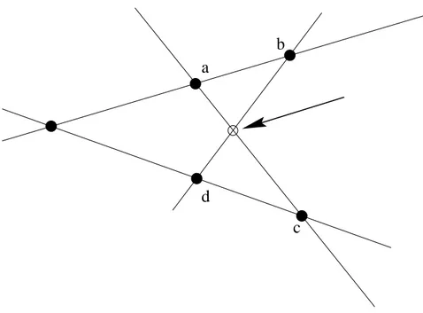
Definition 1.3.10. A projective space (P, L, I) is a linear space in which the following axioms are satisfied:
(i) (Veblen-Young) If a, b, c, d ∈ P are distinct points, then
ab ∩ cd 6= ∅ ⇒ ac ∩ bd 6= ∅;
(ii) any line is incident with at least three points; (iii) there are at least two lines.
A finite projective space is a projective space in which the set of points is finite.
Definition 1.3.11. A projective plane (P, L, I) is a projective space in which any two lines intersect.
Definition 1.3.12. The dimension of a projective space P = (P, L, I) is the number dim P := inf{|U| : U ⊆ P and U = P } − 1.
a
c
d
b
Figure 1.1: Veblen-Young configuration
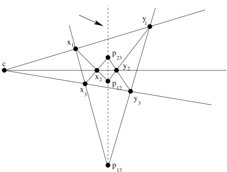
Definition 1.3.13. Six distinct points xi, yi with i ∈ {1, 2, 3} in a linear space (P, L, I)
consti-tute a Desargues configuration if
(i) there exists c ∈ P such that (xi, cyi) ∈ I and (yi, cxi) ∈ I for all i;
(ii) no three of the points c, x1, x2, x3and c, y1, y2, y3are collinear;
(iii) the points pij := xixj ∩ yiyj are collinear.
Definition 1.3.14. A projective space (plane) P is Desarguesian if, for any choice of six points satisfying (i) and (ii) of the Desargues configuration, condition (iii) holds.
Definition 1.3.15. Six distinct points gi, hifor i ∈ {1, 2, 3} in a linear space (P, L, I) constitute
the Pappus configuration if (i) the gi are all collinear;
(ii) the hi are all collinear;
(iii) the line G := g1g2 meets the line H := h1h2in a point c that is distinct from any of the gi
and any of the hi;
(iv) given qij := gihj∩ gjhi, then (q12, q13q23) ∈ I.
Definition 1.3.16. A projective space (plane) P is Pappian if, for any choice of six points satisfying conditions (i), (ii) and (iii) of Pappus configuration, condition (iv) holds as well.
c x x x y y y p p 1 1 2 2 3 3 p 12 13 23
Figure 1.2: Desargues configuration
Theorem 1.3.17. Any projective space of dimension at least 3 is Desarguesian. Still, there exist non-Desarguesian projective planes.
Theorem 1.3.18 (Hessenberg). A finite projective plane P is Pappian only if it is Desarguesian.
1.3.2 Algebraic constructions
Theorem 1.3.19. Let K be a division ring and let V be a (left) vector space over K of dimension
n ≥ 3. Then, the triple (P, L, ⊆) where
(i) P is the set of all 1-dimensional (left) vector subspaces of V , (ii) L is the set of all 2-dimensional (left) vector subspaces of V , (iii) ‘⊆’ is the natural inclusion,
is a Desarguesian projective space of dimension n − 1.
Definition 1.3.20. The symbol P(V ) is used to denote a projective space constructed from a vector space V as in Theorem 1.3.19.
Theorem 1.3.21 (Projective derivation of a vector space). Let V be a vector space of dimension
n ≥ 3 over a field K. Define
(i) 0 := (0, . . . , 0) ∈ V ; (ii) V? := V \ {0};
c
g
g
g
h
h
h
G
H
q
q
q
1 2 3 1 2 3 12 13 23Figure 1.3: Pappus configuration (iii) Vibe the set of i-dimensional subspaces of V ;
(iv) P := V?/K? := {T \ 0 : T ∈ V
1};
(v) L := {X
K? : X ∈ V2}.
Then, PV := (P, L, ∈) is a (n − 1)-dimensional Pappian projective space which is isomorphic to P(V ).
Definition 1.3.22. Let PVnbe the projective derivation of a vector space V of dimension n over
a field K. Then, V is the underlying vector space of (P, L, ∈). The projection map P :
½
V? → V?/K?
x → [x] := K?x
is called the projectivisation of V .
Theorem 1.3.23. Let V be a vector space over a division ring K; then P(V ) is Pappian if and
only if K is a field.
Definition 1.3.24. The symbol PG(n, K) := PKn+1 ' P(Kn+1) denotes the Pappian
projec-tive space obtained by projectivisation from a vector space of dimension n + 1 over K.
Definition 1.3.25. Let (P, L, I) = PG(n, K) be a Pappian projective space. For any given t such that −1 ≤ t ≤ n, the symbol PGt(n, K) denotes all projective subspaces of PG(n, K)
Theorem 1.3.26 (First representation theorem). Given any Desarguesian projective space P of
dimension n, there exist a division ring K and a vector space V of dimension n + 1 over K such that P is isomorphic to P(V ).
Corollary 1.3.27. Let P be a Pappian projective space of dimension n. Then, there exists a
field K such that P ' PG(n, K).
Proof. By Theorem 1.3.18, P is Desarguesian; Theorem 1.3.26 guarantees that P = P(V ),
with V a vector space of dimension n over a division ring K; by Theorem 1.3.23, K is a field. Hence, P ' PG(n, K).
Corollary 1.3.28. Let P be a finite projective space of dimension at least 3. Then, P is Pappian.
Proof. From Theorem 1.3.17, P is Desarguesian; hence, P = P(V ) for some vector space V
over a finite division ring K; by Theorem 1.2.2, K is a field. It follows that P is isomorphic to PG(n, q) := PG(n, K). Hence, P is Pappian.
Theorem 1.3.29 (Tecklenburg). A Desarguesian finite plane is Pappian.
This result can be proved as in Corollary 1.3.28 or in a more direct geometric way, as done in [Tec87]. Due to Theorem 1.3.23, this is equivalent to Wedderburn’s result.
1.3.3 Morphisms
Definition 1.3.30. Let V be a vector space over a field K and let σ be an automorphism of K. A semi-linear automorphism of V with companion automorphism σ is a bijection θ from V into
V such that, for all x, y ∈ V and g ∈ K:
(i) θ(x + y) = θ(x) + θ(y); (ii) θ(gx) = gσθ(x).
Theorem 1.3.31 (Second representation theorem). For any collineation φ of a Desarguesian
projective space (P, L, I) = P(V ), there exists a semi-linear automorphism θ of V that induces φ, in the sense that for all x ∈ P ,
φ(x) := {θ(t) : t ∈ x}.
Definition 1.3.32. Let P = P(V ) be a Desarguesian projective space. A projectivity of P is a collineation of P induced by a linear map of the underlying vector space V .
Definition 1.3.33. Let φ be a collineation of the projective space PG(n, K). A point p ∈ PG(n, K) is a centre of the collineation φ if
(ii) any line L through p is fixed by φ.
A hyperplane H of PG(n, K) is an axis of the collineation φ if φ|H is the identity.
Theorem 1.3.34. A non-trivial collineation φ of PG(n, K) has at most one centre and one axis;
furthermore, φ has a centre if and only if φ has an axis.
Definition 1.3.35. A collineation φ is central (or axial) if it has a centre. A central collineation
φ whose centre is incident with its axis is called an elation; if the centre of φ is not incident with
its axis, then φ is called a homology.
Definition 1.3.36. The set of all collineations of the Pappian projective space PG(n, K) is denoted by the symbol
PΓL(n + 1, K); the set of all projectivities of PG(n, K) is written as
PGL(n + 1, K).
Theorem 1.3.37. For all integers n ≥ 1 and for all fields K, the set PΓL(n + 1, K) together
with mapping composition constitutes a group. The set of all projectivities of PG(n, K) is a subgroup of PΓL(n, K).
Theorem 1.3.38. Let K be a field, n ≥ 1 and GL(n + 1, K) be the group of all non-singular
matrices of dimension (n + 1) × (n + 1) over K. Then,
PGL(n + 1, K) ' GL(n + 1, K)/K?.
Definition 1.3.39. The stabilizer of a line of PG(n, K) in PGL(n + 1, K) is the affine linear
group AGL(n, K).
1.3.4 Singer cyclic groups
Singer cyclic groups have been introduced in [Sin38].
Definition 1.3.40. A Singer cyclic group of a projective space Π is a collineation group that is cyclic and transitive on the points of Π. A generator of a Singer cyclic group is a Singer cycle. Definition 1.3.41. A projective space Π is cyclic if it admits a Singer cyclic group.
Lemma 1.3.42. Any Desarguesian projective space PG(n, q) is cyclic.
Lemma 1.3.43. Any Singer cyclic group is transitive on the set of the lines of PG(2, q).
Lemma 1.3.44. Any Singer cycle of PG(n, q) is conjugate to a diagonal linear transformation
1.4 Polynomials and matrices
The results in this section are taken from [Lan80] and [HH70].
1.4.1 Definitions
Definition 1.4.1. Let K be a field. By the symbol Mat(n, K) we denote the ring of all n ×
n matrices with entries in K. For any prime power q, the ring Mat(n, GF(q)) is written as
Mat(n, q).
For any given matrix M ∈ Mat(n, K), we write its transposed matrix, obtained interchang-ing rows and columns of M, as M?.
Definition 1.4.2. Two matrices A, B ∈ Mat(n, K) are equivalent if there exist a matrix C ∈ Mat(n, K), such that
(i) det C 6= 0; (ii) A = CBC?.
Definition 1.4.3. Given any matrix M ∈ Mat(n, K), its characteristic polynomial CM(x) is
CM(x) := det(M − xIn),
where Inis the identity matrix in Mat(n, K).
Definition 1.4.4. For any matrix M ∈ Mat(n, K) and any polynomial p(x) =Ppixi ∈ K[x],
the valuation of p(x) at M is
p(M) :=XpiMi.
Lemma 1.4.5. Let M ∈ Mat(n, K); the set
J(M) := {p ∈ K[x] : p(M) = 0} is an ideal of the ring K[x].
Since K[x] is a principal ideal domain, there exist a generator element for J(M) that is unique up to multiplication by elements of K?.
Definition 1.4.6. The minimal polynomial of M ∈ Mat(n, K) is the monic generator MM(x)
of the ideal J(M) of K[x].
Lemma 1.4.7. For any M ∈ Mat(n, K), (i) deg CM(x) = n;
(ii) CM(x) ∈ J(M);
(iii) MM(x) divides CM(x).
Definition 1.4.8. The null space of a matrix M ∈ Mat(n, K) is the set Null M of all vectors
x ∈ Knsuch that
Mx? = 0.
Equivalently, the null space of M is the kernel of the homomorphism induced by M. The null
space of a polynomial p(x) with respect to a matrix M is the set
NullM p(x) := {y ∈ Kn: p(M)y? = 0}.
1.5 Varieties over finite fields
The few general algebraic geometry results presented in this section are from [Ful69]. Ref-erences for the GF(q)-case are [Hir98b] and our notes [Hir98a]; the conventions adopted are those of [Hir98b].
1.5.1 Polynomials as functions over projective spaces
For any field K, we shall denote by Rnthe ring Rn(K) := K[X1, . . . , Xn] of polynomials in
n indeterminates with coefficients in K. This ring is the free ring generated by the symbols X1, . . . , Xnover K.
Definition 1.5.1. Let K be a field; a form f of degree r in n + 1 variables is a homogeneous polynomial f ∈ K[X0, . . . , Xn] of degree r.
Definition 1.5.2. We denote the set of all forms in n + 1 variables over a field K by Rn(K) ⊆
K[X0, . . . , Xn]; the set of all forms in n + 1 variables of given degree r over K is written as
Rrn(K).
Let f ∈ Rn(K) be a form, and let V be an n + 1-dimensional vector space over K; for any
vector v = (v0, . . . , vn) ∈ V ' Kn+1, the value of f at v is the scalar
f (v) := f (v0, . . . , vn).
Remark 1.5.3. Neither Rn(K) nor Rrn(K) are subrings of Rn[X0], since the former is not
closed under the sum and the latter under the product. On the other hand, (Rn(K)?, ·) is a
monoid and (Rrn(K) ∪ {0}, +) is a group.
Lemma 1.5.4. Let P = PG(n, K) = PKn+1 be a projective space and consider a form f ∈
Rn(K). Then, for all v ∈ Kn+1\ {0}, f (v) = 0 implies
Proof. Since z ∈ Pv, there exists a λ ∈ K? such that z = λv. Denote by r be the degree of f ;
then,
f (λv) = λrf (v) = 0.
1.5.2 Algebraic sets and ideals
Definition 1.5.5. Let K be a field and assume F := {f1, . . . , fk} ⊆ Rn(K). The set of zeros
determined by F is
V(F) := V(f1, . . . , fk) := {Pv ∈ PKn+1: f1(v) = f2(v) = . . . = fk(v) = 0}.
The ideal of F in Rn(K) is denoted by
I(F) := I(f1, . . . , fk).
Lemma 1.5.6. Let F, F0 ⊆ R
n(K), with I(F) = I(F0). Then,
V(F) = V(F0).
Remark 1.5.7. Lemma 1.5.6 shows that the set V(F) does not depend on the list of forms F but only on the ideal F generates in Rn(K).
Definition 1.5.8. Let K be a field and assume F = {f1, . . . , fr} to be a set of forms in Rn(K).
The projective variety defined by F is the pair
F(F) := F(f1, . . . , fr) := (V(F), I(F)).
The set I(F) is the ideal of F(F).
Definition 1.5.9. The intersection of two varieties F(F) and F(G) is the projective variety
F(F) ∩ F(G) := F(F ∪ G).
Definition 1.5.10. A sub-variety of a variety F(F) is a projective variety F(G) such that
F(G) ∩ F(F) = F(G).
Lemma 1.5.11. Let F(F) and F(G) be two projective varieties. Then,
F(F) ∩ F(G) = (V(F) ∩ V(G), I(F ∪ G)).
Definition 1.5.12. Let F = {f1, . . . , fr} ⊆ Rn(K) be a set of forms over a field K. A
K-rational point of F(F) is an element Pv ∈ V(F) ∩ PG(n, K).
Let K denote the algebraic closure of K. A point of F(F) is any P t ∈ PKn+1 such that
f (t) = 0, for all f ∈ F. The set of all points of F(F) is
V(F).
Definition 1.5.13. An algebraic set Y in PG(n, K) is a set of points of PG(n, K) such that there exists F ⊆ Rn(K), with
Y = V(F).
The ideal of the set Y is defined as
˜I(Y ) := I(F).
1.5.3 Number of rational points: zeta functions
Definition 1.5.14. Let X = V(F) be a projective variety over a finite field GF(q). A point P t of X of degree i is a point that is GF(qi)-rational, but is not GF(qj)-rational for any j < i.
A closed point of degree i is a set
P t := {P tσ : σ ∈ Gal(GF(qi) : GF(q))} = {P t, P tq, . . . , P tqi−1},
where P t is a point of X of degree i.
Definition 1.5.15. A divisor on a curve X = V(F) is an element of the free group generated by all its closed points.
The group of all divisors of X is written as Div(X).
Definition 1.5.16. A divisor D is a K-divisor if all its components are K-rational points. Remark 1.5.17. A divisor D on a curve X = V(F) is a formal sum
D = X
P t∈V(F)
nP tP t,
where
(i) nP t ∈ Z;
(ii) nP t = 0, for all but a finite number of P t;
(iii) if P t is a point of X of degree i, then nP t = nP t0, for all P t0 ∈ P t.
Definition 1.5.18. Let X = V(F) be a projective curve; its zeta function is the formal series
ζX(T ) :=
X
D∈DivK(X)
Tdeg(D).
Lemma 1.5.19. For any projective curve X = V(F) defined over GF(q), let (i) Nibe the number of points of X that are GF(qi)-rational;
(iii) Bj be the number of closed points of degree j. Then, (i) ζX(T ) = 1 + ∞ X s=1 MsTs; (ii) Ni = X j|i jBj; (iii) ζX(T ) = ∞ Y j=1 (1 − Tj)−Bj = exp( ∞ X i=1 NiTi/i).
1.5.4 Dimension and algebraic sets
Lemma 1.5.20. The family of the algebraic sets of PG(n, K) is closed under finite union and
intersection; both ∅ and PG0(n, K) are algebraic sets.
Definition 1.5.21. The Zariski topology on PG0(n, K) is the topology whose open sets are the
complements of algebraic sets.
Remark 1.5.22. Any sub-variety F(G) of a projective variety F(F) is closed in F(F).
Definition 1.5.23. A non-empty subset Y of a topological space Ξ is irreducible if it cannot be expressed as the union Y1∪ Y2of two proper subsets, each one of which is closed in Y with the
induced topology.
The empty set is not irreducible.
Definition 1.5.24. The dimension of a topological space Ξ is the supremum of all the integers i such that there exists a chain
Z0 ⊂ Z1 ⊂ . . . ⊂ Zn = Ξ
of distinct irreducible closed subsets.
Definition 1.5.25. The dimension of a variety F(F) is the topological dimension of its point set V(F), when endowed with the Zariski topology.
Remark 1.5.26. The null form 0 ∈ Rn(K) defines the projective variety
F(0) := (PG0(n, K), {0}).
Its topological dimension is n, the same as the incidence dimension of PG(n, K). This is the only variety of dimension n in PG(n, K).
Definition 1.5.27. Let F(F) be a variety. By
Fr(F)
we denote the set of all r-dimensional sub-varieties of F(F).
Definition 1.5.28. An hypersurface of PG(n, K) is a projective variety of dimension n − 1 in PG(n, K). A 3-dimensional projective variety is a projective surface; a 2-dimensional projec-tive variety is a projecprojec-tive curve.
1.5.5 Non-singular varieties
Definition 1.5.29. Let F = {f1, . . . , fk} ⊆ Rn(K). The Jacobian matrix associated to F at a
point p ∈ Kn+1is the k × (n + 1) matrix J
F(p) given by (JF(p))i(j+1) := ∂Fi ∂Xj ¯ ¯ ¯ ¯ p , where (i) 0 ≤ j ≤ n; (ii) 1 ≤ i ≤ k;
(iii) ∂Fi/∂Xj is the formal derivative of Fi with respect to Xj.
Definition 1.5.30. A variety F(F) is non-singular at a point p ∈ V(F) if the rank of its Jacobian matrix JF(p) at p is maximal, that is
rankJF(p) = (n − dim F(F)).
A variety F(F) is non-singular if it is non-singular at each of its points.
Definition 1.5.31. Assume Px to be a non-singular point of a variety F(F). The tangent space to F(F) at Px is the subspace of PG(n, K) generated by the points corresponding to the pro-jection of the rows of the Jacobian matrix JF(x).
1.6 Unitary Groups
The results in this section are taken from [Die71] and from the notes of the 1999 Socrates Summer school [Kin99].
1.6.1 Definitions
Let V be a vector space over a field K and assume σ to be either an involution of K or the identity mapping; denote by K0 the subfield of K fixed by σ.
Definition 1.6.1. A sesquilinear form f defined on V is a mapping V × V → K such that, for any choice of x, x1, x2, y, y1, y2in V and λ in K,
(i) f (x1+ x2, y) = f (x1, y) + f (x2, y);
(ii) f (x, y1+ y2) = f (x, y1) + f (x, y2);
(iii) f (xλ, y) = λσf (x, y);
(iv) f (x, yλ) = f (x, y)λ.
Definition 1.6.2. Let f and g be two sesquilinear forms which are respectively defined over the vector spaces X and Y . Then, f and g are equivalent if there exists an isomorphism T of X into Y such that, for any x, y ∈ X,
f (x, y) = g(T x, T y).
Definition 1.6.3. A sesquilinear form f defined on V is non-degenerate if, for any non-zero vector x ∈ V , there exists a vector y ∈ V such that
f (x, y) 6= 0.
The form f is reflexive if, for any x, y ∈ V ,
f (x, y) = 0 ⇐⇒ f (y, x) = 0.
Definition 1.6.4. A sesquilinear form f is Hermitian if, for any x, y ∈ V ,
f (x, y) = f (y, x)σ.
From now on we assume f to be a sesquilinear form on V which is both non-degenerate and reflexive.
Definition 1.6.5. A transformation u of V unitary with respect to the form f is any bijective linear transformation of V which preserves f . That is, for any x, y ∈ V ,
f (x, y) = f (u(x), u(y)).
Lemma 1.6.6. The set of all transformations of V unitary with respect to the form f form a
Definition 1.6.7. Let θ be an automorphism of the field K. A unitary semi-similarity of V
(corresponding to the form f and the automorphism θ) of multiplier ru is a collineation u :
V → V such that, for any x, y ∈ V ,
f (u(x), u(y)) = ruf (x, y)θ.
Lemma 1.6.8. The set of all unitary semi-similarities of V forms a subgroup ΓUf(n, K) of the
group ΓL(n, K) of all collineations of V .
Definition 1.6.9. A semi-similarity u is linear if the automorphism θ associated with u is the identity of K.
Lemma 1.6.10. The set of all linear semi-similarities is a subgroup GUf(n, K) of the general
linear group GL(n, K); indeed,
GUf(n, K) = ΓU(n, K) ∩ GL(n, K).
Lemma 1.6.11. Let f , g be two equivalent sesquilinear forms. Then, the unitary groups induced
by f and g are all isomorphic; that is, Uf(n, K) ' Ug(n, K), ΓUf(n, K) ' ΓUg(n, K) and
GUf(n, K) ' GUg(n, K).
Definition 1.6.12. Let α be in K?. The dilation of V with coefficient α is the mapping
hα :
½
V → V x → xα.
Lemma 1.6.13. The set H(n, K) := {hα : α ∈ K?} of all dilations of V is a normal subgroup
of ΓL(n, K).
Definition 1.6.14. The group of all projective collineations of the projective space PV , obtained by derivation from V , is the quotient group
PΓL(n, K) := ΓL(n, K)/H(n, K). The canonical projection from ΓL(n, K) in PΓL(n, K) is denoted as
P : ½
ΓL(n, K) → PΓL(n, K)
x → xH(n, K).
Definition 1.6.15. The projective collineation groups
PΓUf(n, K), PGUf(n, K), PUf(n, K)
are defined as the images in PΓL(n, K) via the projection P of ΓUf(n, K), GUf(n, K), Uf(n, K).
1.6.2 Subspaces and forms
Lemma 1.6.16. A necessary and sufficient condition for the existence of a unitary
transforma-tion u, mapping a subspace X ≤ V into Y ≤ V , is that the restrictransforma-tion of the form f to X is equivalent to the restriction of the same form f to Y .
Definition 1.6.17. A subspace X of V is orthogonal to Y ≤ V with respect to the form f if and only if, for all x ∈ X and y ∈ Y ,
f (x, y) = 0.
The largest subspace of V orthogonal to X is denoted as
X⊥:= {v ∈ V : ∀x ∈ X, f (v, x) = 0}.
Definition 1.6.18. A space X is isotropic if X ∩ X⊥ 6= {0}; it is totally isotropic if X ⊆ X⊥.
Definition 1.6.19. An hyperbolic plane X is a non-isotropic plane of V containing at least one isotropic vector.
Lemma 1.6.20.
(i) If X and Y are two totally isotropic subspaces of V and dim X = dim Y , then there exists
an u ∈ Uf(n, K), such that u(X) = Y .
(ii) There exists an integer ν such that any totally isotropic subspace of V is contained in a
totally isotropic subspace of maximal dimension ν.
Definition 1.6.21. A quasi-symmetry (with hyperplane H) is a unitary transformation u fixing point-wise a non-isotropic hyperplane H in V .
Definition 1.6.22. A hyperbolic transformation is a unitary transformation u ∈ Uf(n, K) fixing
all vectors of a subspace Y ≤ V of dimension n − 2 which is orthogonal to an hyperbolic plane. Remark 1.6.23. The projective image PX of an hyperbolic plane X is a hyperbolic line. A
pro-jective hyperbolic transformation is, hence, a unitary transformation fixing all points belonging
to a projective hyperplane (PX)⊥.
1.6.3 Hermitian groups
Definition 1.6.24. A Hermitian sesquilinear form g is a trace form if, for all v ∈ V , the element
g(v, v) ∈ K can be written as a trace over K0; that is, for any v ∈ V , there exists a λ
v ∈ K such
that
Lemma 1.6.25. If the characteristic of K is not 2, then all Hermitian sesquilinear forms over
K are trace forms. If K has characteristic 2, then the only trace forms are the alternating ones.
Definition 1.6.26. The standard Hermitian product on the vector space V is the Hermitian sesquilinear form h·, ·i, given by
h·, ·i :
½
V × V → K
(u, v) → Puiviσ.
For any Hermitian form g equivalent to the standard Hermitian product, the unitary groups Ug(n, K), GUg(n, K), ΓUg(n, K) and PUg(n, K), PGUg(n, K), PΓUg(n, K), are denoted
omitting the reference to g; that is, they are simply written as U(n, K), GU(n, K), ΓU(n, K) and PU(n, K), PGU(n, K), PΓU(n, K).
For any prime power q, the notation U(n, q) := U(n, GF(q)) will be adopted as well.
1.6.4 Generators of the unitary group
Theorem 1.6.27. Let f be a non-alternating symplectic form. Then, either the unitary group is Uf(n, K) = U(2, 4), or Uf(n, K) is generated by the quasi-symmetries of V ' Kn.
Theorem 1.6.28. Let ν be the dimension of a maximal totally isotropic subspace X of V . Then, (i) if ν ≥ 1, all the transformations in Uf(n, K) are products of hyperbolic transformations;
(ii) if ν ≥ 1 and n ≥ 3, all non-isotropic lines are the intersection of two hyperbolic planes,
except in the case where Uf(n, K) coincides with the orthogonal group O(3, 3).
1.6.5 Morphisms and automorphisms
Define Z(n, K) as the centre of GL(n, K).
Lemma 1.6.29. For any sesquilinear form f , the following isomorphism relations are satisfied: (i) PGL(n, K) ' GL(n, K)/Z(n, K);
(ii) PΓUf(n, K) ' ΓUf(n, K)/H(n, K);
(iii) PGUf(n, K) ' GUf(n, K)/Z(n, K).
Theorem 1.6.30. Suppose g to be a Hermitian form, let n ≥ 3 and assume charK to be odd.
Then, all automorphisms of the unitary group Ug(n, K) can be written as
φ(u) = χ(u)ug,
(i) g ∈ ΓUg(n, K);
(ii) χ is an homomorphism of Ug(n, K) into its centre.
Theorem 1.6.31 (Walter). Let K be a field of odd characteristic with more than 3 elements and
assume n ≥ 5. Then, any automorphism of the projective unitary group PUf(n, K) is obtained
from an automorphism of Uf(n, K) by way of quotienting.
1.7 Hermitian Forms and Hermitian varieties
The main references for this section are [Seg67], [Seg65] and [Hir98b].
1.7.1 Hermitian matrices
Assume K to be a field with an involutory automorphism σ and let K0 be the fixed field of σ in
K.
Definition 1.7.1. Let H ∈ Mat(n, K). Then, H is (i) Hermitian with respect to the automorphism σ, if
H? = Hσ;
(ii) anti-Hermitian with respect to the automorphism σ, if
H? = −Hσ;
(iii) unitary with respect to the automorphism σ, if
Hσ = (H?)−1;
(iv) anti-orthogonal with respect to the automorphism σ, if
Hσ = H−1.
Lemma 1.7.2. The conjugate of a Hermitian matrix via a unitary matrix is a Hermitian matrix. Lemma 1.7.3. Let H ∈ Mat(n, K) be a Hermitian matrix; then, det H ∈ K0.
Proof. Since det H = det H?,
d := det H = det H? = det Hσ = (det H)σ = dσ.
Definition 1.7.4. Let V be a vector space over K, and assume H ∈ Mat(n, K) to be a matrix, Hermitian with respect to the automorphism σ. The σ-Hermitian form over V defined by H is the form
h :
½
V × V → K
(x, y) → xσHy?.
Lemma 1.7.5. Assume q to be a square and let H ∈ Mat(n, q) be a Hermitian matrix. Then,
αH is a Hermitian matrix for any α ∈ GF(√q).
Definition 1.7.6. A polynomial f (x) in K[x] is Hermitian if and only if, for any integer n and any Hermitian matrix H ∈ Mat(n, K), f (H) is a Hermitian matrix.
Remark 1.7.7. All polynomials with coefficients in the subfield K0 of K are Hermitian.
Lemma 1.7.8. The set of all Hermitian matrices of Mat(n, q) is a vector space of dimension n2
over GF(√q).
Proof. A Hermitian H matrix can be given by providing the entries in its upper triangular part;
any entry on the main diagonal, that is of the form Hii, is an element of GF(√q); entries above
the main diagonal are elements of GF(q); hence, they have the form a + ²b with a, b ∈ GF(√q)
and ² a fixed element of GF(q) \ GF(√q).
A direct count shows that exactly
n + 2(1
2n)(n − 1) = n
2
choices of elements of GF(√q) have to be made in order to determine H.
Definition 1.7.9. Two matrices A, B ∈ Mat(n, K) are Hermitian-equivalent if there exists a non-singular matrix C ∈ Mat(n, K) such that
A = CσBC?.
Theorem 1.7.10 (Equivalence of Hermitian matrices). Let H ∈ Mat(n, K) be a Hermitian matrix of rank n − t. Then, H is Hermitian-equivalent to a matrix J of the form
J := diag(j0, . . . , jn−t, 0, . . . , 0| {z } t times
),
where ji ∈ K0 for any i.
1.7.2 Hermitian forms
Lemma 1.7.11 (Representation theorem for Hermitian forms). Let V be a vector space of dimension n over the field K and let H be a Hermitian matrix in Mat(n, K). Then, the σ-Hermitian form over V defined by H is a sesquilinear σ-Hermitian form in the sense of Definition
1.6.4. Conversely, given a sesquilinear Hermitian form h over a vector space V of dimension n, there exists a Hermitian matrix H ∈ Mat(n, K) such that h is the σ-Hermitian form over V defined by H.
Thanks to Lemma 1.7.11, it is possible to identify σ-Hermitian forms and sesquilinear Her-mitian forms.
Remark 1.7.12. Over an arbitrary field K, there might exist different classes of Hermitian forms, depending on the involutory automorphism σ of K which has been chosen. On the other hand, if K is a finite field GF(q), then there is an involutory automorphism of K if and only if
q is a square. In this case, the involution is unique and it is associated with the subfield of K
with index 2, that is GF(√q).
Let q be a prime power p2n. The unique involutory automorphism σ of GF(q) over GF(√q)
will be denoted by the conjugation sign. Namely, for x ∈ GF(q):
x := xσ = x√q.
Definition 1.7.13. Let r ≥ 1 be an integer and assume V to be a vector space of dimension n over the field K. A mapping h : Vn → K is a homogeneous polynomial mapping of degree r if
there exists a polynomial f ∈ Rrn(K) such that
h :
½
Vn → K
(p1, p2, . . . , pn) → f (p1, p2, . . . , pn).
Such a polynomial f is said to represent the mapping h.
For a vector space V over an arbitrary field K, a σ-Hermitian form h usually cannot be represented by a polynomial mapping. For instance, there is no polynomial in R2n(C) which
represents the Hermitian form induced over the vector space Cn by the standard Hermitian
product between complex numbers. However, if K is finite, the following theorem is true. Theorem 1.7.14. Let V be a vector space of dimension n over GF(q), with q a square, and
let h be a Hermitian form defined over V . Then, there exists a polynomial f ∈ R√2nq+1 which represents h.
Proof. The only involution of GF(q) is the Frobenius automorphism σ : t → t√q. Theorem
1.7.11 guarantees that there exists a Hermitian matrix H such that the form h is represented by
H. Then,
h :
½
V × V → K
(x, y) → x√qHy?.
By computing the expansion of the vector/matrix product, this yields
h(x, y) = n X j=1 [yj n X i=1 x√i qHji],
1.7.3 Hermitian hypersurfaces: definitions
This subsection deals only with Hermitian forms which are representable by polynomials. How-ever, the assumption that the field K is finite is not necessary.
Definition 1.7.15. The Hermitian hypersurface defined by the Hermitian form h is the algebraic variety
H(h) := F(f (x, x)),
where f is a polynomial representing h and x = (X0, . . . , Xn). The Hermitian hypersurface
defined by the matrix H is the Hermitian hypersurface H(H) := H(h),
where h is the Hermitian form induced by the matrix H. The algebraic variety F(0), induced by the trivial Hermitian form, is not considered to be a Hermitian variety
Remark 1.7.16. A Hermitian form h over GF(q) is not a Hermitian form over GF(qi) for i > 1.
However it makes sense to consider the GF(qi)-rational points of the GF(q)-Hermitian variety
H(h).
Theorem 1.7.17. The set of all Hermitian hypersurfaces of PG(n, q) can be endowed with the
structure of a PG(n2+ 2n,√q).
Proof. The correspondence in Lemma 1.7.11 allows us to identify Hermitian forms with
Hermi-tian matrices. Let H, H0 be two non-zero Hermitian matrices defining the same Hermitian
hy-persurface, and call f, f0the Hermitian polynomials associated with them. Since F(f (x, x)) =
F(f0(x, x)), the ideals generated by f (x, x) and f0(x, x) have to be the same, that is
I(f (x, x)) = I(f0(x, x)).
It follows that there exists an α ∈ GF(q)?such that
f (x, x) = αf0(x, x).
Then, by construction,
H = αH0
and α ∈ GF(√q)?. An immediate computation shows the converse, namely that if H = αH0
with α ∈ GF(√q), then H(H) = H(H0).
By Lemma 1.7.8, the Hermitian matrices in Mat(n + 1, q) constitute a vector space V over GF(√q) with dimension (n + 1)2.
Distinct Hermitian hypersurfaces of PG(n, q) are in one-to-one correspondence with el-ements of the set U of all Hermitian polynomials modulo GF(q)?; the set U, in turn, is in
one-to-one correspondence with the quotient space
V?/ GF(√q)?,
which is isomorphic to PG(n2+ 2n,√q) and this proves the theorem.
Definition 1.7.18. The rank of a Hermitian hypersurface
H(H) := F(xHx?)
is the rank of the matrix H.
Lemma 1.7.19. A point x on a Hermitian hypersurface H(H) is singular if and only if x belongs
to the null-space of H, that is
xH = 0.
Lemma 1.7.20. A Hermitian hypersurface is non-singular if and only if the matrix associated
with it has full rank, that is, it is a non-singular matrix.
Lemma 1.7.21. Let H and H0 be two Hermitian-equivalent matrices. Then, the hypersurfaces
H(H) and H(H0) are projectively equivalent.
Lemma 1.7.22. For any k ≤ n+1, there exists exactly one Hermitian hypersurface in PG(n, q)
of rank k up to projectivities.
Proof. Theorem 1.7.10 and Lemma 1.7.21 imply that any non-singular Hermitian hypersurface
in PG(n, q) is projectively equivalent to the one generated by the diagonal matrix
M := diag(m0, . . . , mk, 0, . . . , 0),
where m0, . . . , mk are in GF(√q). Since the norm from GF(q) onto GF(√q) is surjective,
there exist elements ti ∈ GF(q), such that
titi = mi.
Let T be the matrix
T := diag(t0, . . . , tk, 0, . . . , 0).
Then, M is Hermitian-equivalent via T to the block matrix diag(Ik, 0, . . . , 0| {z }
n + 1 − k times
), where Ikis the k × k identity matrix.
Definition 1.7.23. The canonical Hermitian hypersurface of rank k in PG(n, q) is the Hermi-tian hypersurface
Πn−k−1Uk,q
induced by the matrix diag(Ik+1, 0, . . . , 0) ∈ Mat(n + 1, q). The canonical non-singular
Her-mitian hypersurface in PG(n, q) is the non-singular HerHer-mitian hypersurface Un:= Π−1Un,q := H(I),
where I is the identity of Mat(n + 1, q).
A Hermitian hypersurface which is projectively equivalent to a Πn−1U0,q is a hyperplane
repeated√q + 1 times; a Hermitian hypersurface projectively equivalent to a Πn−k−1Uk,q is a
Hermitian cone having as vertex a Πn−k−1 ∈ PGn−k−1(n, q) and base a Uk,q.
Definition 1.7.24. The canonical Hermitian norm of rank k in PG(n, q) is the form
hk,n(x) := k X i=0 xixi = k X i=0 x√i q+1.
With Definition 1.7.24, we can write (i) Un:= F(hn,n(x));
(ii) Πn−k−1Uk := F(hk,n(x)).
1.7.4 Hermitian sub-varieties and points
Lemma 1.7.25. The intersection of a Hermitian H variety with a subspace Πr ∈ PGr(n, q) of
dimension r not completely included in H is a Hermitian variety of Πr.
Corollary 1.7.26. The intersection of a Hermitian variety with a line is either a line, a Baer
subline or a point.
Proof. The corollary follows by observing that Hermitian varieties in dimension 1 are either
Baer sublines or lines (if completely degenerate), while a Hermitian variety in dimension 0 is a point.
The following theorems deal with the cardinality of the set of the points of a (possibly singular) Hermitian variety H.
Theorem 1.7.27. The zeta function of the non-singular Hermitian curve U2,qis
ζU2,q(T ) =
(1 +√qT )q−√q
Theorem 1.7.28. The number of GF(q)-rational points of the non-singular Hermitian variety Un,q is µ(n, q) := [q(n+1)/2+ (−1)n][qn/2− (−1)n]/(q − 1). Corollary 1.7.29. (i) µ(1, q) =√q + 1; (ii) µ(2, q) = q√q + 1; (iii) µ(3, q) = (q + 1)(q√q + 1).
Theorem 1.7.30. The singular Hermitian variety ΠmUk,q contains:
(i) qm+ qm−1+ . . . + 1 = (qm+1− 1)/(q − 1) singular points;
(ii) qm+1µ(k, q) non-singular GF(q)-rational points;
(iii) η(m, k, q) = (qm+1− 1)/(q − 1) + qm+1µ(k, q) total GF(q)-rational points.
1.7.5 Hermitian varieties and unitary groups
The stabilisers of a Hermitian variety Un,q in the collineation groups of PG(n, q) are unitary
groups. In fact, the following lemma holds true.
Lemma 1.7.31. The stabiliser in PGL(n + 1, q) of the set of the GF(q)-rational points of Un,q
is PGU(n + 1, q). The stabiliser of the same set in PΓL(n + 1, q) is PΓU(n + 1, q).
Definition 1.7.32. The group PγU(n + 1, q) is the group of all collineations of PG(n, q) sta-bilizing the point set of Un,q which are associated either with the identity of the field GF(q) or
with its involutory automorphism.
Lemma 1.7.33 (Orders of groups). Assume p be a prime, and let q = ph, with h even; define
λ²(m, r) := rm(m−1)/2 m
Y
i=1
(ri− ²i).
Then, the collineation groups have the following orders:
(i) | GL(n + 1, q)| = λ1(n + 1, q);
(ii) | PGL(n + 1, q)| = (q − 1)−1λ
1(n + 1, q);
(iii) PGU(n + 1, q) ≤ PγU(n + 1, q) ≤ PΓU(n + 1, q); (iv) | PGU(n + 1, q)| = λ−1(n+1,√q)
√