Experimental and numerical characterization of heating domestic appliances for energetic efficiency improvement

UNIVERSITY OF SALERNO

DEPARTMENT OF INDUSTRIAL ENGINEERING

Ph. D. Thesis in Mechanical Engineering

XIII Cycle N.S. (2011-2014)

“Experimental and numerical characterization of heating

domestic appliances for energetic efficiency improvement”

Ing. Antongiulio Mauro

Supervisor Coordinator

Ch.mo Prof. Ciro Aprea Ch.mo Prof. Vincenzo Sergi Co-tutor

“Start where you are,

Use what you have,

Do what you can.”

This thesis work is subject to a three years embargo, any content of this thesis work has restricted access and must not be published without author

Table of contents

INDEX OF FIGURES IV

INDEX OF TABLES VIII

NOMENCLATURE 1

INTRODUCTION 8

CHAPTER 1: EUROPEAN DIRECTIVES ON BOILER EFFICIENCY 10 CHAPTER 2: BOILER ENERGY BALANCE AFFECTED BY MEASUREMENT

UNCERTAINTY 12

2.1 Boiler space heating efficiency characterization 12

2.2 Efficiency measurement and uncertainty 17

2.3 Indirect efficiency measurement uncertainty 24

2.4 Energy balance closing 26

2.4.1. Statistical based energy balance closure using z-test 28

2.4.2. Measurement system design 30

CHAPTER 3: RISK ANALYSIS ON EFFICIENCY DECLARATION 32

3.1 Water heating efficiency 32

3.2 Space heating seasonal efficiency 35

3.3 Surveillance process 37

3.3.1. Safety margin on efficiency 40

CHAPTER 4: PRODUCTS CHARACTERIZATION AND EFFICIENCY

IMPROVEMENT 43

4.1 Insulation improvement for tanks and Boilers 43

4.1.1. Boiler losses 46

4.1.2. Tank losses 46

4.1.3. Thermal camera measurements 49

4.2 Boiler tank draw-off analytical model 52

CHAPTER 5: EXPERIMENTAL AND NUMERICAL STUDIES FOR NEW

PRODUCTS FEASIBILITY 56

5.1 Conventional boiler for Erp 56

5.1.1. Boiler methane combustion 57

5.2 Ultramodulating condensing boilers 62

5.2.1. Annual gas consumption calculation 63

5.2.2. Stationary efficiency model identification 66

5.2.3. Boiler working conditions definition 68

5.2.4. Boiler cycling efficiency and ERC 69

5.2.5. Annual electricity consumption calculation 74

5.2.6. Ultramodulation consumption analysis 75

5.3 Ultramodulationg boiler modeling results 79 5.4 Electrical-gas consumption trade-off for optimal modulation 81 5.5 Savings deriving by electrical resistance adoption 83 5.6 Correlation between savings and day degrees 84

ACKNOWLEDGEMENTS 88

Index of figures

Figure 1. Example of boiler cycling to satisfy a load lower than minimum heat output. _________________________________________ 17 Figure 2. Boiler efficiency measurement apparatus, instruments label

refers to Table 2. ______________________________________ 18 Figure 3. Relative weight of different measurements on the heat input

and heat output uncertainty_____________________________ 21 Figure 4. Transient measurement comparison between a 1mm

thermocouple and a 3mm thermoresistance ________________ 23 Figure 5. Thermocouples positioning with surface methods. ________ 23 Figure 6. Comparison of direct and indirect estimation of efficiency in

terms of measurement uncertainty _______________________ 24 Figure 7. Relative weight of losses terms on the global heat loss of a

boiler _______________________________________________ 25 Figure 8. Advantages and disadvantages of input/output method (direct)

and energy balance method (indirect) for efficiency estimation (ASME, 2013). ________________________________________ 26 Figure 9. Comparison of the statistical distribution of heat input and

global heat output measurements ________________________ 30 Figure 10. Measurement system design criteria based on statistical

closure of energy balance. ______________________________ 31 Figure 11. Laboratory and production effects on water heating and space

heating efficiencies uncertainty __________________________ 38 Figure 12. Surveillance on declared data process schematization. ____ 40 Figure 13. Surveillance tollerance on water efficiency analysis on storage boiler assuming an acceptable risk of non-conformity. ________ 41 Figure 14. Surveillance tollerance on water efficiency analysis on storage

Figure 15. Insulation measurement test rig composed by electrical resistance and pump controlled by PID in order to deliver constant temperature water ____________________________________ 44 Figure 16. B represents the test bench loss characterization while A the

DUT measurement test. ________________________________ 45 Figure 17. Boiler standby losses results for three differently insulated

boilers ______________________________________________ 46 Figure 18. Boiler frontal thermal camera measurement during burning

phase and correspondent Matlab elaboration ______________ 49 Figure 19. Boiler burner/tank logic scheme for sanitary draw-off ____ 52 Figure 20. Experimental and model water temperature draw-off for a

22kW and 40liters storage boiler and a 10l/min flow rate.

Experimental draw-off show firstly a peak due to tank temperature stratification and following a valley, whereas modeled temperature maintains an average value _____________________________ 54 Figure 21. Experimental and modeled specific flow rate is reported for

different tapped water quantities for a 22kW and 40 liters storage boiler. Model well approximates SR experimental results. _____ 54 Figure 22. Boiler combustion loss as a function of oxygen concentration

in the flue gas, which is correlated to the air excess. __________ 58 Figure 23. Ostwald triangle for methane – The triangle correlate air

excess “e” with CO, CO2 and O2 concentrations determining the

combustion conditions. ________________________________ 59 Figure 24. Boiler efficiency increase due to condensation as a function of

water return temperature and heat input __________________ 60 Figure 25. Model overview: on the top model inputs and on the right the

model output. Model is composed by different sub-models: bins model, house loads calculation, plant model and boiler

Figure 26. Satistical frequency distribution of external temperatures during considered heating periods for the Italian cities of Belluno, Bologna, Roma, Salerno and Palermo. _____________________ 66 Figure 27. Boiler efficiency experimental, modeled and relative error.

Boiler delta water temperature is fixed and equal to 20°C. Data are divided into modulation and ultra-modulation range. _________ 68 Figure 28. Boiler efficiency reduction from stationary conditions due to

cycling losses (ERC) as a function of the external temperature for a fixed boiler and different building specific losses. ____________ 73 Figure 29. Experimental and modeled fan electrical consumption and

relative error for different fan rpm and modulation ratio. Data is divided into modulation and ultra-modulation range. _________ 75 Figure 30. For a boiler with maximum modulation ratio equal to 10: in

top figure the efficiency degradation due to cycling losses, in the second one, boiler heat output and loads as a fuction of external temperature. _________________________________________ 76 Figure 31. For a boiler with maximum modulation ratio equal to 20: in

top figure the efficiency degradation due to cycling losses, in the second one, boiler heat output and loads as a fuction of external temperature _________________________________________ 77 Figure 32. For a boiler with maximum modulation ratio equal to 40: in

top figure the efficiency degradation due to cycling losses, in the second one, boiler heat output and loads as a fuction of external temperature. _________________________________________ 78 Figure 33. Optimal maximum modulation ratio as a function of electrical power for different Italian cities. _________________________ 82 Figure 34. Model results and relation between degree days and total

energy saving due to ultra-modulation for different building specific heat losses.____________________________________ 84

Figure 35. Typical heat demand and correlation with days degree for different European countries. (De Rosa M., 2014)____________ 85

Index of tables

Table 1. Efficiency requirements of central heating boilers _________ 11 Table 2. Instruments characteristics and measurement uncertainty __ 19 Table 3. Relative and absolute uncertainty on heat output, heat input

and water efficiency ___________________________________ 22 Table 4. Hypothesis test on energy balance closing for a 22kW boiler. 29 Table 5. Example of three tapping profiles for sanitary water efficiency

determination (Erp) ___________________________________ 33 Table 6. Water heating energy efficiency classes of water heaters

organized by declared load profiles (Erp) ___________________ 34 Table 7. Water heating energy efficiency bans for different load profiles

(Erp) ________________________________________________ 35 Table 8. Seasonal space heating efficiency classes (Erp) ____________ 36 Table 9. Laboratory and production uncertainty contribution on water

heating and seasonal space heating efficiency ______________ 39 Table 10. Tank heat loss measurement for two different insulation

material and a volume of 40 liters ________________________ 48 Table 11. Heat losses measurement of the different sides of a 22kW

boiler using thermography and correspondent relative efficiency point. _______________________________________________ 50 Table 12. Comparison of heat loss measurement methodologies for an

40 liters insulated tank _________________________________ 51

Table 13. Indirect efficiency, Heat input, CO ppm and CO2 % for an

increased performance standard boiler supposing no jacket loss. 61 Table 14. Degree- days (DD) allowable daily heating period and climatic

zone for five Italian cities. _______________________________ 65

Table 15. Electrical EpYear and gas consumption CYear as a function of the

maximum modulation ratio MR, delta consumptions δ_PE and δ_EPE

Nomenclature

eq

H

MR, calculation for a fixed building and MR

.

Q heat (kW)

_

h tank equivalent thermal loss (W m-2K-1)

.

V volumetric flow rate (m3 s-1)

A area (m2)

alpha statistical significance level bcc boiler compensation curve

eq

H calculation for a fixed building

C gas consumption (kWh)

c specific heat capacity (kJkg-1K-1)

CC primary energy coefficient of conversion (-)

cf boiler cycling frequency (h-1)

CH central heating

CO2 carbon dioxide

CR cooling coefficient (W m-1s)

DD degree day (kWh)

e air excess (%)

E electrical energy (kWh)

ERC efficiency reduction coefficient (-) Erp Energy related products regulation

Ex statistical expected value of random variable F correction terms to seasonal efficiency (%)

f generic function

G20 methane

G21 Methane family gas limit G231 Methane family gas limit

GCV gross calorific value (MJ m-3)

h occurrence (h)

H specific heat loss (W K-1)

L house load (kWh)

mass mass quantity (kg)

MR maximum modulation ratio (-)

mr modulation ratio (-)

N total bins number (-)

NOx nitrogen oxides

P electrical power (kW)

p pressure (kPa)

PLR partial load factor (-)

q normalized losses (-)

Q thermal energy (kWh)

R2 Coefficient of correlation

S/V surface volume ratio (m-1)

SCF smart control ratio

SF specific flow rate

smart smart function compliance

ss sample size

t time (s) Ultramodulation modulation ratios higher than 10

V Volume (m3)

var statistical variance

Z statistical z-value

Gas reference conditions: temperature= 15°C, pressure= 1013.25 mbar

Greek Symbols

∆ absolute variation

η efficiency

σ population standard deviation

δ relative variation or differential partial variation

a convective-radiative heat exchange coefficient (W m-2 K)

ρ density (kg m-3)

Subscripts

stbyls standby heat thermal losses

%dry percentage of dry flue

acc acceptable

air air related quantity

b boiler

bench test bench related quantity

c control

C critical

cold cold water

d distribution

DUT device under test

e external

eb electronic board

el electrical

elec electrical consumption for hot water production

elr electrical resistance related quantity

em emission

EPE electrical primary energy

eq equivalent

fa forced air

fan fan

fl flue losses

fr firing

fuel fuel consumption for hot water production

g global

H2O water

i index

ign ignition related quantity

in input

j jacket

k discretization index

load load

min minimum

na natural air flow

nc normal cooling

nom nominal conditions

ON on

Op optimal

out output

output water output and losses

p primary energy

PE total primary energy

postp post purge

prep pre purge

pump pump

r return

ref reference conditions

room room

s stationary

seas seasonal space heating efficiency

tank tank related quantity

unc uncertainty

Introduction

.Equation Chapter 1 Section 1

Every year 5 million of boilers for domestic heating are sold in the European Union (EU). Because heating contributes to more than 20% to the whole energy use in the EU (Karsten D. H., 2000), strategies for energy saving are of great interest and have been widely explored.

Currently in the European Union efficiency requirements on boilers are becoming more and more stringent: following the common target of the energy reduction, European directives 2005/32/EC on the eco-design of energy-using products and 2009/125/EC on the energy-related products, oblige the labeling of central heating (CH) boilers in performance categories. Furthermore, EU policy is to phase out appliances with low performance, by no longer giving the right to be sold on the European market. The regulation “Erp” ( European Commission, 2013) which enters into force from 26th of September 2015 sets efficiency bans so that low efficiency boilers are going to be excluded from EU market. As a consequence, boilers manufacturers should develop products to meet regulatory requirements and perform a wide experimental mapping covering the whole product range. Manufacturers have to face significant investments to adopt appropriate facilities in terms of technical specifications and testing capability. Robust measurements become necessary to establish correct performance categories and not generate conflicts with surveillance bodies. Additionally, an efficiency oriented product development could be necessary to improve or strengthen the positioning in energetic ranking. At the same time, experimental activities oriented to establish products phase-out becomes necessary.

In the present PhD thesis work, carried out at Ariston Thermo Group in Osimo R&D center, experimental and modeling activities have been performed and reported concerning heating appliances.

Concerning domestic methane supplied gas boilers, a comprehensive analysis of energy fluxes has been carried out, different methods for efficiency estimation have been compared with related measurement uncertainties (ASME, 2013). Existing testing protocol and standards have been considered for efficiency determination and investigation (LABNET, 1998) (CEN , 2013).

The boiler energy balance closing problem has been undertaken through a novel statistical approach.

Subsequently, insulation testing methods have been set-up and compared, in particular an automated test rig has been constructed and compared to thermal camera measurements.

Experimental investigation have been undertaken in order to improve products efficiency with respect to Erp ban, analyzing products limitations.

Concerning boiler efficiency, it has been showed that installing condensing high efficiency boilers rather than standard ones, improve control management and rightsizing boiler capacity (Heselton K. E., 2000.) (Heslton K. E., 1998) produce a great effect on boilers energy consumption and efficiency on field.

Furthermore the boiler modulation is an important parameter in order to rightsize the boiler as well as to minimize fuel consumption (Lazzarin, 2014).

Most of the domestic gas boilers on the market provide space heating below nominal capacity within a range described by the modulation ratio. This parameter expresses the maximum heat output reduction in respect to the nominal one. Currently the typical modulation ratio available on the market is equal to 10 for the top class condensing boilers, which means for a 22kW nominal heat output a minimum output of 2.2 kW.

Experimental evidences underline that boiler efficiency significantly varies from the nominal value when boiler works in partial load (Verma V.K., 2013) or in cycling conditions (Verma V.K., 2013). Yet, high modulation ratios could improve efficiency by reducing cycling frequency, nevertheless would improve boiler operating times and electrical consumption. The real convenience of adopting ultra-high modulation ratio is currently under investigation. (Marcogaz, 2013) Finally, in the present thesis a stationary bin model has been presented in order to simulate boiler behavior on field for different cities, buildings and plants and investigate the convenience of adopting ultra-high modulation ratios. A stationary bin method base model was performed in order to investigate advantages and limitations for such boilers.

1.

CHAPTER 1: European Directives on

boiler efficiency

Considering the replacement of standard boilers with condensing ones it is theoretically possible to reach energy saving of the order of 10-15%; this fact has led to a number of European initiatives to phase out poor efficiency boilers from the market.

Energy labeling for electrical appliances (EU directive 92/75/EC, which is from July 2011 replaced by Directive 2010/30/EU) has been found to be a successful tool to promote energy efficient appliances in the market. Efficiency requirements in connection with CE-labeling of gas-fired boilers are mentioned in Directive 92/42/EC. This was later modified through Directive 2004/8/EC. Moreover, other more recent European directives are important for CH boiler performance. The energy performance of buildings directive (EPBD) 2002/91/EC resulted in many countries introducing new minimum requirements for boiler efficiency accompanied by regular mandatory inspections of the boilers (Kessen, 2007).

In the past, the European commission had taken initiatives to remove boilers with very poor efficiency from the market with the purpose of reducing energy use and emissions. The European Commission developed a new approach through directive 92/42/EEC, later converted into national legislation (Kessen, 2007). Boilers have to satisfy essential requirements before being introduced into the market and put into service, such as the requirements indicated in Table 1.

Type of boiler

Efficiency requirements for full load (

out_nom .

Q )

Efficiency requirements for 30% part load (0.3 out_nom . Q ) Mean temperatur e of the water [°C]

Requirements (in%) Mean temperatur e of the water in the boiler [°C] Requirements (in%) Standard boiler 70 ) Q 2log( 84 _{out_nom} . + ≥ 50 80 3log(Qout_nom) . + ≥ Low temperatur e boiler 70 ) Q 1.5log( 87.5 out_nom . + ≥ 40 87.5 1.5log(Qout_nom) . + ≥ Gas-fired condensing boiler 70 ) Q log( 91 out_nom . + ≥ 30 97 log(Qout_nom) . + ≥

Table 1. Efficiency requirements of central heating boilers

The _{out_nom}

.

Q is the nominal heat output of the boiler which corresponds to the maximum heating capacity. Notified Bodies have been nominated by member governments and notified by the European Commission to investigate the conformity of CH boilers and water heaters to the requirements of the directive mentioned above; tests could be performed by the notified body or an accredited agency according to ISO 17025. There have been national labeling, boiler database and information systems implemented to promote high efficiency boilers such as BOILSIM in Denmark and SEDBUK in UK.. (Kessen, 2007). The present version of Directive 2005/32/EC on the ecodesign of Energy using Products (EuP) and 2009/125/EC on the energy-related products (Erp) oblige the labeling of central heating boilers: a classification of the CH boilers into different categories is proposed. Commission Regulations (EU) No 811/2013, 812/2013, 813/2013, 814/2013 implement Directive 2009/125/EC clarifying technical aspects of ecodesign and energy labeling processes. In the present work, directive 2009/125/EC and related regulations are generally referred to as “Erp” regulation.

Erp regulation is going to become effective as of the 26th of September 2015.

2.

CHAPTER 2: Boiler energy balance

affected by measurement uncertainty

2.1

Boiler space heating efficiency characterization

. cl . fl . j . out in . Q Q Q Q Q = + + + ( 1 ) Where _in .

Q is the heat input, Q._jthe jacket losses,

. fl

Q the flue losses,

. out

Q the heat output and

. cl

Q the cycling losses.

In case of stationary behavior so that no cycling effects occur, heat output '

Q

.

out and boiler efficiency ηs can be defined: . fl . j in . . out' Q (Q Q ) Q = − + ( 2 ) in . . out s Q ' Q η = ( 3 )

The heat output could be also expressed as heat provided to water:

. r f _ H2O . . out' ρV c(T T ) Q = − ( 4 )       − = 2 ) c(T ) c(T c_ f r ( 5 )

Where ρ and c are interpolated value of the water density and specific heat, supposed functions of water temperature T only; ρ _{is dependent on} the temperature of the section where the water flow rate H2O

.

V is measured. The specific heat

_

c is calculated as the arithmetic mean between temperatures T and_f T , which are the flow and return temperatures of the _r water, according to standard nomenclature (CEN , 2013).

The heat input _in

.

Q is equal to methane chemical power and can be calculated as follows: GCV V p p T T Q . gas ref gas gas ref in . = ( 6 )

Where GCV is the higher calorific value per volume in gas reference conditions, V._gas the gas flow rate,

ref gas gas ref p p T T

is the volume correction ratio related to reference conditions of the calorific value. Losses terms could be expressed as follows:       _{⋅ + ⋅ ⋅ −} ⋅ =V (V c− V c ) (T T ) Q _%dry fl_dry _%wet fl_wet _{fl air}

. gas . fl ( 7 )

Where V_%dry and V_%wetare respectively the percentages of dry and wet flue gases related to gas flow, cfl_dryand cfl_wet the mean specific heat, T_fl

the flue discharge temperature and T_airthe air temperature. The jacket losses could be expressed as follows:

(

)

(

)

∫∫

∑

Where α is the radiative-convective coefficient, T is the jacket j

boiler jacket, M the size of surface discretization and k a discretization index.

Referring to equation 3, by measuring losses terms and heat input it is possible to evaluate boiler efficiency indirectly:

s in . . fl . j s_ind η Q Q Q 1 η = − + = ( 9 )

So defined indirect stationary efficiency is mathematically equal to efficiency η_s.

The ηs could be considered as a “direct” way to evaluate efficiency and

in the present work will be also noted as follows :

s dir η

η = ( 10 )

When considering cycling behavior

. cl

Q ≠0, an average long time efficiency can be defined for the boilerη_b, where

. out Q is equal to: . cl . j fl . in . out Q Q Q Q Q = − − − ( 11 ) Dividing by . in Q : . in . cl . in . . j fl . in . out Q Q Q Q Q 1 Q Q −             + − = ( 12 )

The boiler efficiency can be written as follows: cl

s b η q

η = −

( 13 )

reduction coefficient (ERC) could be then defined as the ratio between boiler efficiency and steady state efficiency.

ERC η η q 1 η η _s s cl s b =      − = ( 14 ) Where: s b η η ERC = ( 15 )

This ratio expresses the boiler efficiency degradation due to on-off cycling behavior.

The ratio between the load

. load

Q and the minimum heat output Q. _{out_min} , determinates cycling frequency (cf_b), this ratio is defined as partial load ratio PLR: . out_min . load Q Q PLR = ( 16 )

So that the cycling frequency could be considered as a function of PLR only:

f(PLR) cf_b =

( 17 )

In particular when the boiler is oversized compared to the load (PLR<1),

b

cf increases reducing the ERC. Indeed: When PLR<1,ERC<1

When PLR≥1,ERC=1 ( 18 )

Moreover, the external temperature influences cycling losses because it affects heat losses during off periods (Bonne U., 1985). As a

consequence, ERC can be than considered as a function of the external temperature and of the PLR (Heselton K. E., 2000.) (Heslton K. E., 1998) (Landry R. W. et al., 1993):

) T f(PLR,

ERC = _e ( 19 )

Boiler heat output can be described in terms of modulation ratio (mr):

out . out_nom . Q Q mr = ( 20 )

So that the minimum heat output out_min .

Q is provided at maximum modulation ratio:

max(mr)

MR

=

Thus MR is also defined as:

out_min . out_nom . Q Q MR = ( 22 )

An example of boiler cycling behavior is shown in Figure 1: when the load is lower than heat output, boiler starts on-off cycles at maximum modulation (MR) and flow temperature starts oscillating, in present example MR is equal to 4.

Figure 1. Example of boiler cycling to satisfy a load lower than minimum heat output.

2.2

Efficiency measurement and uncertainty

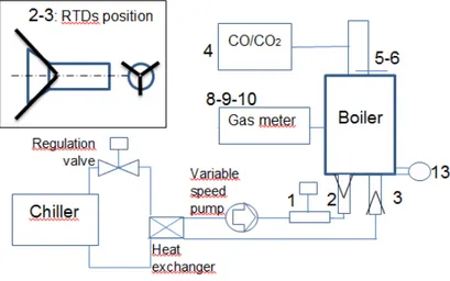
Boiler instantaneous efficiency η_s has been measured according to standard (CEN , 2013) specs using the following experimental apparatus: boiler is operated by an automatic test bench, allocated in a climate chamber with controlled air temperature set to 20+-1°C, with a chiller that dissipates the heat produced. Three RTD PT100 positioned as shown in Figure 2 are used for each water temperature measurement, and an electromagnetic water flow meter positioned in proximity of temperature probes for density interpolation. Volumetric gas counter equipped with an encoder is used for gas volume flow measurement, inlet gas temperature and pressure are measured for volume flow correction to standard

conditions. Cylinders of certified methane G20 99.5% supply the boiler. Air inlet temperature, flue temperature and CO/CO2 emissions are monitored constantly during tests. A monophasic wattmeter was used to measure electrical consumption.

Figure 2. Boiler efficiency measurement apparatus, instruments label refers to Table 2.

Table 2. Instruments characteristics and measurement uncertainty

Efficiency results are the average value of three consecutive ten minutes tests with inter-repeatability within 0.5%.

Referring to equation 2 an error propagation analysis on the efficiency was performed. Using instruments measurement uncertainties reported in Table 2, uncertainty on the efficiency resulted equal to 2.2% at nominal heat output conditions and 80-60 °C flow-return temperature.

N° Measurement Instrument Type u% (2k)

1 Water flow Siemens

MAG1100+MAG6000 Electromagnetic 1.1 2 Temperature flow 3 PT100 3mm, 4wires Thermoresistances 0.1 3 Temperature return 3 PT100 3mm, 4 wires Thermoresistances 0.1

4 CO-CO2 Siemens Ultramat 23 2.0

5 Flue temperature PT100 3mm, 4 wires Thermoresistance 0.5

6 Inlet air temperature PT100 3mm, 4 wires Thermoresistance 0.5

7 Gross calorific value Certified cylinder - 1.0

8 Inlet gas pressure Siemens Sitrans P DS3

Piezoresistive 0.7

9 Inlet gas temperature

PT100 3mm, 4 wires Thermoresistance 0.5

10 Gas flow Elster G4/10 – equipped with encoder

Volumetric+encoder 1.0

11 Air temperature PT100 3mm, 4 wires Thermoresistance 0.5

12 Environment pressure

DeltaOhm HD9408TBARO

Piezoresistive 1.2

In particular, considering the following not correlated error propagation formula for a generic function F:

) x ,..., f(x F= i M ( 23 ) ) var(x x f var(F) i M i 2 i

∑

It is possible to express the variance of the heat output as:

2 r f 2 f r 2 r f f r 2 2 r 2 H2O 2 H2O . H2O . out . ) T (T c ) var(cT ) var(cT ) T (T ) var(T ) var(T ρ var(ρa ρ ) var(T B V ) V var( ) ' Q var( − + + − + + + + = ( 25 )

Considering a linear interpolation for the water density,

H2O H2O H2O B T A ρ= + ( 26 )

While the heat input variance is:

2 2 ref gas gas 2 ref gas gas 2 gas . gas . in . GCV var(GCV) ) T (T ) var(T ) p (p ) var(p V ) V var( ) Q var( + + + + + = ( 27 )

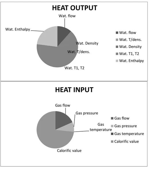
The relative weight of measurement on uncertainty was estimated and reported in Figure 3. The most critical measurements are water temperatures for the heat output and the gas calorific value for the heat input, and particular care should be taken in measuring these quantities. Referring to equation 2, water temperature measurements are carried out using three PT100 probes for each temperature. Gas calorific value could be measured using gas chromatography or by adopting certified cylinders, and in the first case particular care must be taken in order to correctly

observe the gas mixture composition.

Figure 3. Relative weight of different measurements on the heat input and heat output uncertainty

For a 22kW boiler in Table 3 an example of heat input, heat output and Wat. flow Wat. T/dens. Wat. Density Wat. T1, T2 Wat. Enthalpy

HEAT OUTPUT

HEAT INPUT

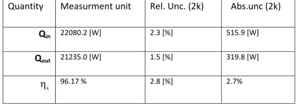
efficiency with relative and absolute uncertainties for a certified calorific value of 2% is reported.

Quantity Measurment unit Rel. Unc. (2k) Abs.unc (2k)

Qin 22080.2 [W] 2.3 [%] 515.9 [W]

Qout 21235.0 [W] 1.5 [%] 319.8 [W]

s

η 96.17 % 2.8 [%] 2.7%

Table 3. Relative and absolute uncertainty on heat output, heat input and water efficiency

By adopting methane certified cylinders with 1% certified uncertainty on GCV it is possible to reduce the heat input uncertainty to 1.6% and the efficiency uncertainty to 2.2%.

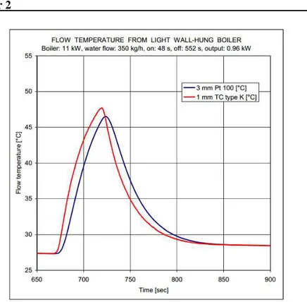
In order to measure water temperature transients, according to EN 13203, three radially staggered 1 mm thermocouples were adopted (Figure 5). Small thermocouples show a quicker response during rapid temperature changes when compared to PT100, accordingly to data in literature and Figure 4. (LABNET, 1998)

Figure 4. Transient measurement comparison between a 1mm thermocouple and a 3mm thermoresistance

2.3

Indirect efficiency measurement uncertainty

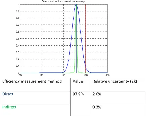
Indirect efficiency analysis is proposed in literature as both an alternative efficiency measurement method and a procedure to verify correct direct efficiency measurements (ASME, 2013). Indirect efficiency method, also known as “energy balance method”, has a generally lower measurement uncertainty when compared to direct efficiency (also known as input output method). This result could apparently be justified assuming that indirect efficiency requires the estimation of the energy loss only, which is a small fraction of the total energy; this results in a limited effect on the overall efficiency uncertainty. For instance, considering 5% of the energy input as losses and a 10% (2k) relative uncertainty on this estimation, the resulting indirect efficiency would be equal to 95%+-0.5%. Comparing error propagation analysis for direct and indirect efficiency, as presented in Figure 6, indirect efficiency shows lower dispersion.

Efficiency measurement method Value Relative uncertainty (2k)

Direct 97.9% 2.6%

Indirect 0.3%

Figure 6. Comparison of direct and indirect estimation of efficiency in terms of measurement uncertainty 85 90 95 100 105 0 0.1 0.2 0.3 0.4 0.5 0.6 0.7 0.8 0.9 1

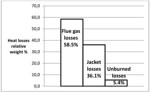
When considering the loss term composition for a full load 60/80 °C test, the most important loss term is related to flue gas, a significant part is relative to jacket loss and a negligible part connected to unburned losses (Figure 7).

Figure 7. Relative weight of losses terms on the global heat loss of a boiler

When measuring efficiency indirectly, not considering or partially considering loss terms implies a boiler efficiency overestimation. Particular care must be taken in order to correctly measure temperature flue gas and inlet air temperature in order to not generate systematic errors. It is evident that jacket loss quantification is critical because of significant relative weight and complex valuation; furthermore, not considering part of the jacket surface would determine systematic overestimation of the efficiency.

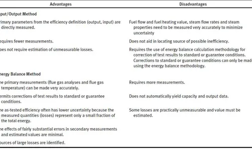
In the following figure advantages and disadvantages of adopting direct and indirect efficiency measurements are reported. Direct measurement is

Flue gas losses 58.5% Jacket losses 36.1% Unburned losses 5.4% 0,0 10,0 20,0 30,0 40,0 50,0 60,0 70,0 Heat losses relative weight %

simpler, directly giving the useful effect quantification yet needs quite accurate measurements; on the other hand, indirect efficiency leads to a very repeatable result and is a useful tool for finding loss causes but needs to complexly estimate small quantities such as jacket loss.

Figure 8. Advantages and disadvantages of input/output method (direct) and energy balance method (indirect) for efficiency estimation (ASME, 2013).

2.4

Energy balance closing

In order to characterize the boiler, energy balance consistence could be checked. The approach undertaken in the present work is not an algebraic verification but a statistical one.

In particular, considering the following energy quantities as random variables: ∆ . output . input . Q Q Q − = ( 28 )

Where input .

Q is an uncertainty affected measurement of _in

.

Q and output .

Q is

the sum of _out

.

Q and _loss

.

Q uncertainty affected measurements, _∆

.

Q is the energy deviation from the energy balance closing.

Considering a sample size equal to ss, the average values are:

_ ∆ . _ output . _ input . Q Q Q − = ( 29 )

The expected value of equation 28 is:

) Q Ex( ) Q Ex( ) Q Ex( _ ∆ . _ output . _ input . = − ( 30 )

So that results in equation 2:

0 ) Q Q ( Q loss . out . in . = + − The variance of _∆ .

Q could be evaluated as follows:

ss σ ss σ sd output 2 input 2 ∆ 2 = + ( 31 )

Population standard deviations

σ

.

Q and output .

2.4.1.

Statistical based energy balance closure using z-test

In order to evaluate the energy balance closing, having considered balance terms as random variables, a z-test could be set up, using statistical approach measurement uncertainties and sample size would be determinant in analysis results despite of using a simple algebraic approach.

A z-value can be defined as follows:

∆ ∆− = 2 . 0 sd Q z ( 32 ) Where Ex(Q ) 0 _ ∆ . = ( 33 )

The following hypothesis test could be formulated: H0: _∆

.

Q = 0 versus H1: _∆

.

Q ≠ 0 ( 34 )

Once established a significance level alpha, the hypothesis test gives as result a p-value.

If the p-value is equal to or smaller than alpha, it suggests that the observed data are inconsistent with the assumption that the null hypothesis is true, and thus that hypothesis must be rejected and the alternative hypothesis could be accepted.

Considering a normalized _ . ∆ Q with respect to _ . input Q : _ input . _ ∆ . _ ∆ . Q Q q = ( 35 )

closing, which is dimensionally an efficiency deviation.

Considering an alpha level equal to 5% and a sample size equal to 27 for the data shown in Table 4 it follows that zero hypothesis must not be rejected, so that the measurement system uncertainty is too high to discriminate an energy quantity of the order of _∆

.

Q and the balance

closure could be considered satisfied.

input Q . [W] input

σ

σ

The p-value increases with overlapping curves and with increasing uncertainty, which means that using poor measurement systems affected by substantial uncertainties, would result in erroneously considering the energy balance as always being satisfied. On the other hand, a very accurate measurement system would lead to not accept null hypothesis and identify the quantity _∆

.

Q as a balance or systematic measurement error.

Furthermore, lower sample size would increase distributions dispersion, having the same effect of higher measurement uncertainties. In Figure 9 the distribution of energy quantities present in Table 4 is plotted, showing overlapping curves.

Figure 9. Comparison of the statistical distribution of heat input and global heat output measurements

2.4.2.

Measurement system design

When defining the energy measurement system, it is possible to establish the deviation from the energy balance closure that system is able to discriminate by conducting Z-tests according to paragraphs 2.4.1. In particular, once having defined the alpha level, the acceptable energy deviation in absolute terms Q _{_acc}

.

∆ or efficiency points q _acc .

∆ , the p-value

could be calculated for different uncertainty measurement systems. Those measurement systems showing p-values higher than the alpha level, would be able to discriminate energy deviation equal to or higher than the selected Q _{_acc}

.

∆ .

% 75 . 0 _ . = ∆ acc q ( 36 )

And an alpha level of 10%, and maximum relative uncertainty of 3% for the input and output energy terms, referring to Figure 9, show that only measurement systems contained in the box could be accepted.

Figure 10. Measurement system design criteria based on statistical closure of energy balance.

As previously described, increasing sample size would have the same effect of improve measurement systems. The proposed methodology is not strictly connected to boilers energy balance yet could be applied to others energy closure problems.

3.

CHAPTER 3: Risk analysis on efficiency

declaration

3.1

Water heating efficiency

Erp regulation defines for water heating appliances a water heating efficiency as follows: cor elec fuel ref wh Q smart) SCF )(1 Q CC (Q Q η + ⋅ − ⋅ + = ( 37 )

Where the Qref depends on the selected water heating tapping profile, Qfuel and Qelec are the fuel and electrical consumption necessary to satisfy the profile, Qcor an ambient correction term:

(

)

(

)

k − ⋅ −

−

= 1

Q_cor ( 38 )

Where k is dependent on the tapping profile, SCF and smart are respectively the smart control factor and the smart compliance ( European Commission, 2013). Table 5 reports as an example part of three daily tapping profiles (sizes M, L and XL), in particular for the hours from 19:00 to 21:45. Complete daily tapping profiles cover one day (h 00-24).

Table 5. Example of three tapping profiles for sanitary water efficiency determination (Erp)

An energy class could be identified, depending on the profile and on the water heating efficiency result, as shown in the following table.

Table 6. Water heating energy efficiency classes of water heaters organized by declared load profiles (Erp)

Ten energy classes could be identified for a wide range of boilers of water heaters; classes are generally separated by 3 or more efficiency points. Within Erp regulation, a market access ban has been set on efficiency in order to exclude poor efficiency boilers from the market. This ban enters in force with the regulation and becomes more stringent starting in 2017. For an XL sized water heater, the minimum allowed efficiency goes from 30% in 2015 to 38% in 2017 (Table 7).

Table 7. Water heating energy efficiency bans for different load profiles (Erp)

3.2

Space heating seasonal efficiency

For boiler space heating appliances a seasonal space heating efficiency could be written as follows:

(

)

(

)

seas 0.85η 0.15η F F F F

η = + − + + + ( 39 )

Where η_{s_4} and η_{s_1}are respectively the full load stationary efficiency at 60/80 °C of water return/flow temperatures (operating condition 4) and the part load efficiency at 30% of the nominal heat output (operating condition 1). For gas supplied boilers:

3%

F₁ = ( 40 )

(

)

WherePb_el_nom, Pb_el_MR and Peb are respectively the electrical

consumption in conditions 1,4 and boiler standby, _stbyls

.

Q is the boiler heat standby losses (paragraph 4.1.1) and

. ign

Q is the ignition burner consumption. Erp Regulation sets different energy efficiency classes, some of them reachable only using coupled systems (A+, A++, A+++). Furthermore a minimum efficiency ban equal to 86% has been set.

As a consequence, referring to the following table, from the 26th of September 2015, boilers with efficiency class within G and B (lower than 86%) will no longer be allowed to be sold on the EU market.

Erp regulations sets ban on other technical aspects of the products such as noisy level, thermal insulation and pollutant emissions.

3.3

Surveillance process

“For the purposes of assessing the conformity with the requirements (…), Member State authorities shall test a single water heater, hot water storage tank (…) and provide the information on the test results to the authorities of the other Member States. If the measured parameters do not meet the values declared by the supplier within the ranges set out (…), the measurement shall be carried out on three additional water heaters (…) The arithmetic mean of the measured values of these three water heaters, hot water storage tanks, (…) shall meet the values declared by the supplier within the range set out (…).” ( European Commission, 2013) Example of tolerances on regulation surveillance are of 8% for ηseasand

5% both on Qfuel and Qelec concerning ηwh.

A risk analysis has been performed on previously described statistical surveillance process.

Data uncertainty was evaluated considering production and laboratory-related uncertainties. In particular, components and processes most involved in determining boiler efficiency were considered in making assumptions and using experimental data to evaluate their effect on efficiency. Concerning lab-uncertainty, measurement uncertainty was evaluated using error propagation theory for equations 37 and 39, furthermore sources of repeatability factors due to testing method have been considered.

In Figure 11, production related aspects and laboratory factors are listed and associated with ηwhand ηseas. In particular it is clear that aspects

involved in determining water heating efficiency are, also because of the test structure, more numerous and critical, being composed of transients

and temporized phases. For storage products, an additional source of non-repeatability comes from storage related phenomena such as thermal stabilizations and water temperature stratification.

Figure 11. Laboratory and production effects on water heating and space heating efficiencies uncertainty

A calculation was performed in order to quantify production, instruments and test uncertainties, discriminating storage products from non-storage, for water heating and space heating efficiencies. Results are reported in the following table and basically show that

η WH

ηseas

Combustion efficiency line acceptance

Productsensors positioninganduncertainty

Primaryheat exchanger

Secondary heatexchanger

TankInsulation variability

Production uncertainty

Measurement uncertainties

Heatexchangephenomena

Tolerances on tapping

Auxiliary systems and test rigs η WH η seas η WH

global uncertainty is significant. Concerning laboratory uncertainty, this is more critical for water heating measurements, in particular for storage water heaters, where values are reached on the order of 8% (2k). Production effects on efficiency uncertainty prove to be not very influential when compared to laboratory uncertainty. Surveillance lab uncertainty is assumed to be the maximum instrumental allowed by regulation plus test uncertainty.

urel (2k) ηWH ηseas

Lab Instruments 4.0% 3.5%

Instruments + test no storage 6.5%

Instruments + test storage 8.06%

Production and process 1.06% 0.80%

External Lab Max instrumental uncertainty allowed

5.0% 4.0%

Max instrumental uncertainty allowed+ test storage

8.6%

Max instrumental uncertainty allowed + test no storage

7.1%

Table 9. Laboratory and production uncertainty contribution on water heating and seasonal space heating efficiency

3.3.1.

Safety margin on efficiency

Because of uncertainty on efficiency data, in order to avoid conflicts with surveillance bodies the surveillance process itself has been modeled to identify efficiency value safety reductions which could decrease the risk of non-conformity. As reported in paragraph 3.3 and represented in Figure 12 surveillance takes from the market one sample and in case of non-conformity other tree samples.

Products on the market present intrinsic efficiency variability due to production uncertainty and aging effects (such as polyurethane insulation decay). Internal laboratory equipment has a known uncertainty on measurement, while for surveillance laboratories the maximum allowable measurement uncertainty has been considered. The result of the analysis is the statistical distribution of the differences of one sample and another three samples, between internal and surveillance measured efficiency. Statistical difference is then compared to regulation-allowed difference limits in order to determine the risk of non-conformity.

3.3.2.

Safety margin analysis results

Concerning space heating efficiency ηseas, the surveillance tolerance is

equal to 8%, results show that because of the significantly high surveillance margins, the risk of non-conformity is lower than 1%.

Concerning water heating efficiency, regulation currently establish for water heating products two different tolerances in case they are combination heaters (both space and water heaters) or simply water heaters. In the first case surveillance tolerance is equal to the space heating one (8%) while for water heaters it is on Qfuel and Qelec , equal to

5% and results in an approximated 4% surveillance on η_wh.

Regarding combination heaters and risk on water heating efficiency, for storage boilers, as shown in Figure 13, a residual risk of about 1% is pointed out. Considering instantaneous appliances, affected by lower uncertainty than storage ones, the risk level is lower still.

Figure 13. Surveillance tollerance on water efficiency analysis on storage boiler assuming an acceptable risk of non-conformity.

Otherwise, considering a gas storage water heater, because of the more restrictive tolerance (about 4% on the efficiency) the residual risk is of the order of 25% on the first sample and of 12% on three samples measurement. In this case a declaration margin could be necessary.

Figure 14. Surveillance tollerance on water efficiency analysis on storage water heater assuming an acceptable risk of non-conformity.

As a consequence of high measurement uncertainty a significant probability of wrong labeling occurs, especially for borderline data. (Kessen, 2007)

4.

CHAPTER 4: Products characterization

and efficiency improvement

4.1

Insulation improvement for tanks and Boilers

Insulation improvement is one of the mostly effective and simple way to increase boiler efficiency both in water heating, especially for storage products, and in space heating working conditions.

An experimental test bench has been constructed in order to test insulation of boilers according to chapter 9.3.2.3.1.3 of EN 15502-1 standard (CEN , 2013), and tanks according to chapter 9.4.2.1.3.

The bench is composed of an electrical resistance, a variable flow pump and a heat exchanger. Temperature controlled water is blown through the device under test (DUT); air temperature, water flow rate and electrical absorption are monitored. The electrical resistance and the pump are piloted by a PWM signal, an Arduino UNO board was used. Water and room temperatures are measured using 3mm PT100 and thermocouples type T, water flow is measured using a vortex flow meter, electrical power absorption through a monophasic wattmeter.

Temperatures, water flow and electrical measurements were carried out using NI labview and a Compact DAQ acquisition system. Software was developed in Labview in order to manage the different phases of the test, to check stability conditions established by the standard and drive pump and resistance. Hydraulic scheme of the test rig is shown in Figure 15.

Figure 15. Insulation measurement test rig composed by electrical resistance and pump controlled by PID in order to deliver constant temperature water

The test bench has been located in a climate chamber and air temperature was set to 20°C.

The bench heat loss _{bench_loss}

.

Q could be evaluated measuring electrical

DUT Fill out Fill in Pump Electrical resistance

power absorbed by the resistance in order to keep bench at a constant temperature, which is equal to the overall electrical absorption (Qel_meas'

.

) minus others auxiliaries absorptions (pump and electronics) el

. Q . bench_loss . el . el_R . Q Q ' Q − = ( 44 )

After bench characterization, test could be done with DUT and measuring

el_R .

Q .Then the DUT loss is equal to _{el_R}

.

Q minus bench losses and electrical auxiliaries absorption. Care must be taken in regulating the pump in order to work at the same power consumption.

el . bench_loss . el_R . DUT_loss . Q Q Q Q = − − ( 45 )

In Figure 16 a scheme of the test phases is presented.

Figure 16. B represents the test bench loss characterization while A the DUT measurement test.

4.1.1.

Boiler losses

The boiler standby loss _stbyls

.

Q is a measure of boiler radiative-convective losses for an air temperature of 20°C and a water temperature of 50°C. (CEN , 2013) The constructed test rig has been used in order to evaluate boilers standby losses for different products, in Figure 17 results for three boilers are reported.

Figure 17. Boiler standby losses results for three differently insulated boilers

Results show that such tests lead to values between 50 and 70 W and, furthermore, tests generally take a significant amount of time to reach steady and stable results. The need of a climate chamber is evident if considering the typical temperature excursion present in a non-controlled environment over so long a time.

4.1.2.

Tank losses

The constructed test rig was used in order to evaluate tank losses according to EN 15502-1. The test provides that water at a controlled temperature of 65°C must be provided to the tank until some thermal

00 20 40 60 80 100 0 1 2 3 4 5 6 7 8 Q_stbyls[W] Time [h] Boiler A Boiler B Boiler C

stabilization criteria are satisfied. In particular, inlet and outlet temperature difference must be lower than 1 K for more than 15 mins and inlet temperature variation must be within 1 K. Room temperature must be equal to 20°C; some variations are admitted. (CEN , 2013)

After stabilization the tank inlet and outlet are sealed and the tank is left to cool for 24 hours (ttank_test).

After the cooling period the tank water temperature is measured.

Considering a tank volume Vtank and a zero-dimensional model, water temperature cooling down inside the tank could be written as follows:

) T (T V ρc A h dt dT air tank tank H2O tank _ − = ( 46 ) Where _

h represents an equivalent coefficient of heat exchange, which includes convective, radiative and conductive over insulation exchanges. Considering the following equation:

tank_test air tank_24 air tank_0 tank H2O tank _ t T T T T ln V ρc A h         − − = ( 47 )

A cooling coefficient (CR) could be defined as follows:

        − − = = air tank_24 air tank_0 H2O tank tank_test tank _ T T T T ln ρc V t A h CR ( 48 )

And the tank heat loss for 65°C water temperature and air temperature of 20°C could be calculated as follows (CEN , 2013):

45 t T T T T ln V ρc Q tank_test air tank_24 air tank_0 tank H2O tank_loss .         − − = ( 49 )

In Table 10, measurements of tank losses are presented for two different materials, polyurethane and polystyrene for a 40 liters Vtank.

Ttank_0 Ttank_24 tank_loss . Q CR Polyurethane 61.3 38.4 77.4 1.1 Polystyrene 65.0 32.9 99.4 1.38

Table 10. Tank heat loss measurement for two different insulation material and a volume of 40 liters

4.1.3.

Thermal camera measurements

Thermal camera temperature measurements were carried out in order to evaluate heat loss. A Flir thermal camera for R&D purposes was used; boiler and tank surface temperatures were measured. Thermal camera measurements were compared to surface PT100 and thermocouples measurements. A Matlab code was developed in order to calculate from a thermal image the correspondent heat loss. Every pixel of a thermographic image was modeled as a constant temperature radiative convective heat exchange problem. In particular the jacket losses could be estimated as follows:

(

)

∑

The coefficient of convective heat exchange was evaluated using Churchill-Chu and Mc-Adams correlations based on dimensionless numbers. The calculation uncertainty was assumed to be equal to 20% which is derived from the most relevant uncertainty term: the convective heat exchange coefficient. Other sources of uncertainty are the temperature field discretization, emissivity estimation and radiation related approximations, not perpendicularity errors and temperature measurement uncertainty.

Figure 18. Boiler frontal thermal camera measurement during burning phase and correspondent Matlab elaboration

In the following table surface losses calculation are reported for a 22kW boiler: results show that most of the heat loss is on the front and left

surfaces of the boiler, which could be explained by the primary heat exchanger positioning.

The global heat loss for the analyzed boiler, which has no insulation panels, corresponds to about 0.8% efficiency points. The rear side of the boiler was insulated with a 2 centimeter thick black wood panel. (Table 11) Surface Loss [W] Top 13.2 Bottom 20.4 Front 59.6 Lateral left 52.2 Lateral right 27 TOT 172.4

Tot [eff. points] 0.78 %

Table 11. Heat losses measurement of the different sides of a 22kW boiler using thermography and correspondent relative efficiency point.

Measurements comparison

Thermal camera measurements have been compared to electrical power measurement results, and water temperature decrease method for a 40 liters tank. Results are shown in Table 12.

Methodology Heat loss [W]

Difference %

Thermal camera 94.2 -

Water temperature decrease 91.9 2.2

Electrical power 80.9 14.2

Table 12. Comparison of heat loss measurement methodologies for an 40 liters insulated tank

The most reliable and stable result can be obtained using the electrical power method, although this method has some limitations: it cannot be used to measure boiler jacket loss during working conditions and takes a long time. Water temperature decrease method could be used only for tanks and has the advantage of showing exiting water temperature, which is the most immediate and intuitive effect of the lack of insulation. Thermal camera method is in general the quickest way to estimate surface heat loss and it can be used in any working condition but has a significant uncertainty.

4.2

Boiler tank draw-off analytical model

The boiler/tank draw-off modeling is useful to foresee boiler behavior within aspects connected to hot water production capacity and could also be a useful tool for tank-boiler first-order dimensioning.

Tank water distribution is generally a 3D non-stationary mathematical problem which could be solved using tools such as FEA and CFD. Temperature stratification effects, which mostly characterize the water temperature inside a tank, are a spatial phenomenon so that at least two or one-dimensional simulation is necessary. Nevertheless, for some applications, a concentrate parameters tank modeling would be sufficient in order to obtain approximated results.

In the present work an analytical zero-dimensional model of boiler-tank has been performed. Considering Figure 19 the water is supposed to go through the heat exchanger and then into the tank.

Figure 19. Boiler burner/tank logic scheme for sanitary draw-off

Considering the following equations:

) T (T V ρc dt dT V

ρc H2O _{tank_in H2O_out} . H2O tank tank H2O = − ( 51 ) * * . out cold tank_in H2O . H2O t 0_for_t t for_t Q ) T (T V ρc < > 〈 = − ( 52 ) set tank(t 0) T T = = ( 53 ) f T_cold = ( 54 ) Heat exchanger

Tank

Where T_{tank_in}and T_{H2O_out}are the tank temperature of incoming and outgoing water, T_coldthe cold water temperature which is general a known function of the time, t* is the time in which, depending on the boiler control, the burner turns on.

Considering previous equations it is evident that the physical and mathematical connection between T_{H2O_out}and dT_tank is not modeled because derives from stratification effects. Indeed, in the presented model it is assumed that these two temperatures are equal. This means that ideally, draw off temperature is always equal to the mean tank temperature. Thanks to this assumption it is possible to analytically solve equation 51.

The specific flow rate is an important parameter for water heaters performance evaluation in terms of hot water draw-off capacity, this quantity can be expressed as follows:

30 T T 10 dt V ρ F cold _ H2O_out _ 10mins 0 H2O . −         =

∫

T are the mean temperature of the delivered hot water and incoming hot water for a 10min test. For volume tanks small enough to replace the initial content of water during the ten minute test, the SF could be properly approximated using the previously shown model. In Figure 20 and 21 for a 40liters and 22kW storage boiler experimental and model results in terms of T_{H2O_out} and SF are reported.

Figure 20. Experimental and model water temperature draw-off for a 22kW and 40liters storage boiler and a 10l/min flow rate. Experimental draw-off show firstly a

peak due to tank temperature stratification and following a valley, whereas modeled temperature maintains an average value

Figure 21. Experimental and modeled specific flow rate is reported for different tapped water quantities for a 22kW and 40 liters storage boiler. Model well

approximates SR experimental results. 10,000 12,000 14,000 16,000 18,000 20,000 100 120 140 160 180 200 Specific flow rate mass_H2O

Specific flow rate

Portata specifica Modello Portata specifica sperimentale Model Experimental

Experimental Model

Results show that by making the previously reported assumptions, the model is able to foresee average energy inside the storage, providing comparable results in terms of specific flow rate. Stratification effects could be included by adding appropriate experimental based characterizations to the analytical draw-off temperature found.

5.

CHAPTER 5: Experimental and

numerical studies for new products

feasibility

5.1

Conventional boiler for Erp

Conventional boilers are sized in order to not determine condensate formation. Considering the burning process of methane, flue condensation heat represents a significant amount of energy, which corresponds to almost 10% of the total methane chemical energy available. In order to allow boilers to extract this energy amount, a specific design is necessary, especially in terms of heat exchange surface and condensate discharge systems. Condensate indeed is corrosive and, when not correctly evacuated, could lead to quality issues. This leads to adopting a discharge system for condensate evacuation in condensing boilers.

Thus, condensing boilers are generally more efficient than standard boilers but also more expensive and sophisticated. Erp regulation sets a ban limit to the space heating efficiency which is equal to 86%; currently space heating efficiency for standard boilers is of the order of 83%. This means that without any significant product development, standard boilers could no longer be sold in Europe after Erp enters in force. In the present PhD thesis work a technical analysis has been carried out in order to evaluate the possibility of increasing efficiency in conventional boiler enough to satisfy the Erp limitations.