WILL HIGH HOUSEHOLD SAVING
IN CHINA PERSIST?
AN APPLICATION OF THE
CONSPICUOUS CONSUMPTION THEORY
Xiaofen Chen
Truman State University, USA
Lin Zhang
Truman State University, USA
Received: April 20, 2017 Accepted: June 26, 2017 Online Published: September 22, 2017
Abstract
Expanding from Veblen’s conspicuous consumption theory, this paper provides new explanations on China’s household saving behavior. Using provincial level data, it finds evidence that urbanization, increased mobility of the population, and a greater degree of openness all depress household saving, likely through higher conspicuous consumption. This result is robust with different estimators and specifications. Among the conventional explanatory variables, the paper finds support for the permanent income theory, but little evidence for the life cycle theory.
Keywords: conspicuous consumption; household saving Chinese economy; cultural changes; international openness; urbanization; population mobility.
1. Introduction
China’s high national saving has captured much attention recently. As one of the leading current account surplus economies, it has been regarded as a source of the global saving imbalances and partly borne the blame for the 2007 subprime mortgage crisis in the U.S. for supplying cheap funds to the international market. As a component of national saving, household saving in China is also well above the world average. Calculated from the United Nations (UN) database, China’s average gross saving rate between 1992 and 2009 reached 33%, while the world average was only 7.1% during the same period. The attention has sparked an academic enthusiasm for explaining household saving patterns in China, but the findings are mixed on what drives the high saving rates and the implications for the future trend.
Both Cristadoro and Marconi (2012) and Liu and Hu (2013) find evidence for the life cycle theory and the precautionary motive, while Cristadoro and Marconi (2012) also stressed the role of liquidity constraint, as in Zhou (2014), who observed siblings, particularly brothers, as
a resort of informal lending. Using the life cycle framework, Curtis, Lugauer, and Mark (2015) conclude that the higher saving rates are largely driven by reduced family sizes due to the population control policy, and future saving rates may decline as the population ages. However, Chamon, Liu, and Prasad (2013) discovered that the middle aged save the least, contrary to the life cycle theory, and they attribute this abnormality to shrinking public education and healthcare, and privatization of the housing sector. Their findings in relation to the life cycle theory are echoed in Chen (2017b) on the consumption of migrant households, who constitute a large portion of urban households. Similarly, Horioka and Wan (2007) only found weak support for the life cycle and permanent income theories, but contended that the high saving rates will persist provided that income growth remains high. The lack of consensus on the role of the age structure may also be partly due to old people’s desire to leave bequests, as studied by Yin (2012).
While Wang and Wen (2012) maintained that increased housing price coupled with borrowing constraint and demographic changes contributed to higher saving rates, Li, Whalley, and Zhao, (2013) rejected such claims, in favor of a negative association between housing price and household saving. On the precautionary saving side, both Ang (2009) and Feng, He, and Sato (2011) found positive effects of the pension reform on household saving, but the result was reversed when the model was applied to data from India in Ang (2009). The introduction of a cooperative medical insurance scheme seemed to only affect middle income households, according to Cheung and Padieu (2015). Kraay (2000) acknowledged the role of future income growth in rural household saving, but the model performed poorly in explaining urban household saving.
Undoubtedly, the aforementioned papers have provided useful explanations of household saving patterns in China. However, the mixed results of applying the conventional theories suggest that current understanding of the determinants of household saving in China is far from adequate, and alternative explanations are worth exploring. In particular, the existing literature fails to capture recent rapid cultural and social changes in China, which are transforming consumer behavior, and may have brought about fundamental and widespread changes in household saving patterns.
This paper incorporates cultural and social factors in explaining household saving behavior that will shed light on the future trend of household saving in China as well as in other economies that are undergoing similarly transformations. It explores alternative theories on consumer behavior, Veblen’s ([1899] 2007) conspicuous consumption theory in particular, to further explain household saving, since consumption and saving are essentially two sides of the same issue. According to Veblen, consumption is a way to display wealth with the purpose of achieving social status, and population mobility and large communities will enhance the importance of such conspicuous consumption. Although it has suffered criticism in the past, Veblen’s theory is endorsed by recent researchers. For example, Bagwell and Bernheim (1996) derived theoretical conditions under which conspicuous consumption may arise. Dutt (2001) concluded that signaling status through conspicuous consumption is the most convincing motive for relative consumption effects. Both Trigg (2001) and Schor (2007) revisited Veblen’s work and Bourdieu’s (1984) related theories, and countered popular criticism of the conspicuous consumption theory.
The arguments in support of the conspicuous consumption concept are validated by recent empirical studies such as those by Heffetz (2011), who found higher income elasticities for wealth-signaling consumption expenditures, and Danzer, Dietz, Gatskova, and Schmillen (2014), who discovered elevated self-reported socioeconomic status through visible consumption for recent migrants. Guarneros, Narváezy, and Vilar (2001) also observed that urbanization resulted in excessive pursuit of consumption by youth in Mexico. In the existing
literature on household saving, the most closely related research to this paper is a study by Chen (2017a), which extended Veblen’s framework and showed that globalization contributed to the decline in household saving through several channels, including cultural and social interactions, increased population mobility and urbanization, international trade (via facilitating access to status goods) and international financial flows (via alleviating credit constraints).
The logical framework of this paper resembles Chen (2017a), but is applied to provincial level data in China, rather than worldwide cross-country data. It also expanded the explanatory variables, including internal population mobility (represented by passenger traffic turnover), communication intensity (represented by communication volume and per capita telephone units), and the share of state-owned enterprises, a factor of particular importance to China.1 It
finds that income per capita and its growth play important roles in household saving, as in the literature; however, there is little support for the role of the age dependency ratios and thus the life cycle theory. Weak evidence of increased precautionary saving is detected, indicated by the negative effects of government social spending (on education, healthcare, etc.) for rural households and the share of state-owned enterprises for urban households. Most importantly, there is consistent evidence in line with the extended conspicuous consumption framework. As in Chen (2017a), increased international openness (foreign direct investment and international trade volume) are found to depress household saving. Likewise, urbanization, population mobility, and communication intensity also have negative effects on saving to various degrees of consistency. The latter conclusion is unique, however, because in Chen (2017a), the urbanization ratio is dropped through model selection, population mobility is not modeled specifically, and communication intensity is part of the globalization index rather than a separate variable.
The structure of the rest of the paper is as follows. Section 2 examines social and cultural changes in China and their possible effects on household saving. Sections 3 and 4 present formal econometric analyses of factors determining household saving using provincial data, and examine the implications for the future trend of household saving. Section 5 contains final remarks.
2. Cultural and social changes and their effects on household saving
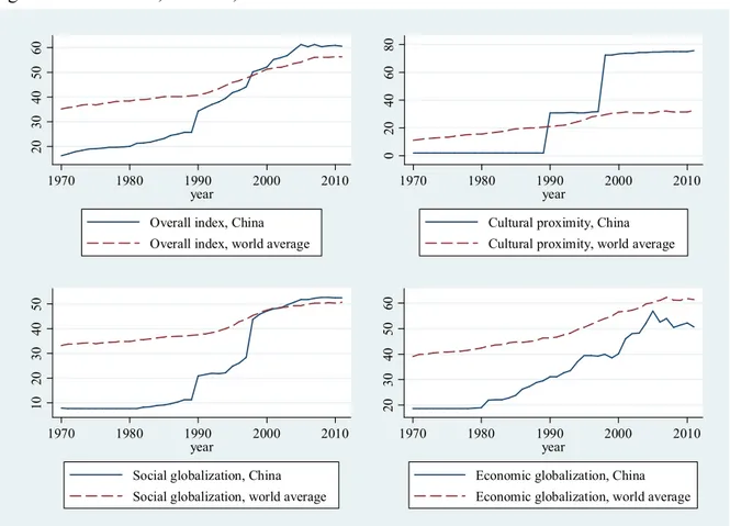
Since the beginning of the economic reform at the end of the 1970s, China has transformed itself from a near-closed status to a remarkably open society, economically, culturally, and socially. Figure 1 shows the degree of globalization in China in comparison with the world average, measured by the KOF globalization index, constructed using economic (36%), social (38%) and political (26%) indicators (Dreher, 2006; Dreher, Gaston, & Martens, 2008). China’s overall globalization index was only about half of the world average in the late 1970s when it embarked its economic reform. By the end of 1990s, its globalization index already surpassed the world average.
Among the components of the KOF globalization index, China’s social globalization index exceeded the world average in the early 2000s; the gap with the world average in the economic dimension has also narrowed greatly. Most markedly, globalization in the cultural dimension, measured by the KOF cultural proximity index, exceeded the world average in the early 1990s and has been far above the average since the late 1990s. The cultural proximity index is constructed using three indicators: per capita number of McDonald’s restaurants (45%), per
1 Some of the variables considered in Chen (2017a) are not included in the model here, either because they
are economy wide variables (for example, interest rate and terms of trade) or are unavailable (for example, corporate saving and household assets).
capita number of Ikea (45%), and trade in books as a percent of GDP (10%). Needless to say, the KOF measure of cultural proximity has its limitations. Nevertheless, in a country with a drastically different traditional culture from the West (including food, drink, and furniture styles), the proliferation of McDonald’s and Ikea undoubtedly reflects Chinese consumers’ willingness to accept and adopt different cultures. As additional evidence, Starbucks also acquired a sweeping presence in China recently.
Figure 1 – Economic, Cultural, and Social Globalization
During the process of globalization, different cultures may influence each other through trading goods and services, exchanging ideas, and consuming each other’s products, particularly cultural products, such as books, movies, and music. As noted by researchers in marketing and management (See, for example, Kim, Forsythe, Gu, & Moon, 2002; Yuan, Song, & Kim, 2011), cultural values are important in shaping life styles and consumer behavior. It follows that influences from other cultures can lead to changes in consumption and saving behavior. As reasoned in Chen (2017a), since the West, represented by the U.S., has a comparative advantage in cultural products, their exports dominate the world market of cultural products. Thus, the influences of Western culture may outweigh those of other cultures. To a society with high initial saving rates, interactions with other cultures that discount the value of frugality may induce behavior changes in favor of higher spending and lower saving. In addition, international trade enables consumers to access more varieties of products, especially luxury goods, which are often perceived as status goods, or goods that can signal or elevate one’s social status, such as iPhones, iPads, and BMW automobiles. Thus, globalization provides additional instruments for conspicuous consumption and hence may exert a negative effect on saving. 20 30 40 50 60 1970 1980 1990 2000 2010 year Overall index, China Overall index, world average
0 20 40 60 80 1970 1980 1990 2000 2010 year
Cultural proximity, China Cultural proximity, world average
10 20 30 40 50 1970 1980 1990 2000 2010 year
Social globalization, China Social globalization, world average
20 30 40 50 60 1970 1980 1990 2000 2010 year
Economic globalization, China Economic globalization, world average
Anecdotal evidence of growing conspicuous consumption is abundant in China. Pursuing luxury brand goods is widespread, especially among urban consumers. Evidence of lavish spending abounds from rising demand for British butlers (Heatley, 2011), to buying luxury cars at costs two to three times the U.S. levels (Goldstein, 2014). Declarations like “rather cry in a BMW than laugh on the backseat of a bicycle”in a reality show is not an isolated incident (Lim, 2012),but an indication of a social phenomenon. Another extreme example is a case where a 17-year-old student willingly sold his kidney to buy an iPad and an iPhone (Guo, 2012).
As noted by many researchers in various fields (for example, Dutt, 2001), East Asia (including China) values collectivism as opposed to individualism. At first sight, conspicuous consumption may seem contradictory to a culture where collectivism is a defining characteristic. However, if social acceptance is not sacrificed, conspicuous consumption can also be rife in a society of collectivism. As a long-term advertising professional who believes that fundamental cultural differences remain between China and the West, Doctoroff (2012) observed that in China, “[l]uxury items are desired more as status investments than for their inherent beauty or craftsmanship.” He noted that luxury brands from abroad are especially desired and consumers are willing to pay high premiums if the products are consumed publicly. Display of luxury brands should ideally be “conspicuously discreet” to meet the need of projecting affluence while “fitting in.” In the meantime, popular products that are consumed privately are often cheap domestic brands, in line with the “conventional virtue” of frugality. His observation coincides with Bagwell and Bernheim’s (1996) theoretical results that “luxury” brands without higher intrinsic value than “budget” brands are priced higher at equilibrium, driven by consumer demand to display wealth.
As additional casual evidence, Japan and South Korea both experienced relatively rapid globalization deepening in the social and cultural dimensions and dramatic decline in household saving in recent years. 2 While the world average of the indicator increased from 33 to 51
between 1970 and 2011, Japan’s social globalization index increased from 26 to 67, and South Korea’s from 22 to 52. In the meantime, Japan’s average gross household saving rate (calculated from the UN’s database) dropped from 21.3% before 1990 to 8.7% after 2000. South Korea’s average net household saving rate plunged from 15.7% before 1990 to just 4.6% after 2000. 3
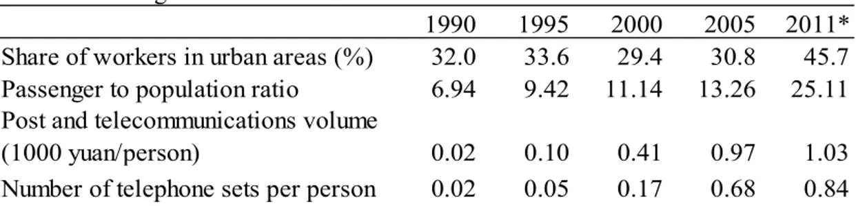
Table 1 – Averages of Provincial Urbanization and Distant Communication Indicators
1990 1995 2000 2005 2011*
Share of workers in urban areas (%) 32.0 33.6 29.4 30.8 45.7 Passenger to population ratio 6.94 9.42 11.14 13.26 25.11 Post and telecommunications volume
(1000 yuan/person) 0.02 0.10 0.41 0.97 1.03
Number of telephone sets per person 0.02 0.05 0.17 0.68 0.84 Source: Calculations from China Data Online and the National Bureau of Statistics of China. * Data for number of telephone sets per person is for 2009.
2 These are the only two East Asian economies in the UN and OECD databases with household saving data
before the 1990s.
3 Source:the OECD database.Gross household saving rate is unavailable for South Korea. The difference
between net and gross saving rates is that the calculation of net saving rate involves subtracting depreciation (consumption of fixed capital) from both saving and disposable income.
China has also undergone other dramatic social changes. First, the speed of urbanization is unprecedented, largely due to high economic growth and the accompanied structural changes. Urban population only accounted for 13.7% of the total population in 1954, and is over 50% in 2011.4 Nearly half of the workers are also in urban areas in 2011 (Table 1).5 Second, population
mobility also increased greatly, although restrictions still remain. Accompanying the increased mobility is the need to communicate through the mail, phones and other means. Table 1 also includes several measures indicating the rapid increase in population mobility and distant communication intensity.
These domestic changes may also have negative effects on saving. In the framework of Veblen’s theory, conspicuous consumption becomes more important when the population is more mobile. This is because in a society with greater mobility, it is more difficult to observe leisure, an alternative means to project wealth; as a result, individuals are forced to rely more on consumption to acquire social repute. Likewise, residing in urban areas boosts the return of conspicuous consumption as one would be more likely to face a large number of transitory observers than in rural and small communities.
The rest of this paper will turn to annual provincial data from China Data Online,6 which
covers all 31 provinces, autonomous districts, and metropolises (all of which may be collectively referred to as provinces hereafter) from 1949 to 2011 (some have shorter coverages). Since provincial data on consumption of fixed capital is not available, net saving rates cannot be calculated. Ideally, both income and consumption should account for non-monetary transactions and transfers as well as goods and services produced for own consumption, and disposable income should adjust for the changes in net equity of households on pension funds (United Nations, 2009). However, due to lack of data, saving rates are calculated as the portion of disposable income that is not used as living expenditure. Three observations associated with unusually high saving rates are dropped, including one for urban households and two for rural households, all with more than 80% saving rates.
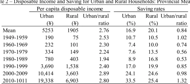
Table 2 – Disposable Income and Saving for Urban and Rural Households: Provincial Means Urban Rural Urban/rural Urban Rural Urban/rural
(¥) (¥) ratio (%) (%) ratio Mean 5253 1905 2.76 16.9 20.1 0.84 1949-1959 190 75 2.53 10.7 10.5 1.02 1960-1969 232 101 2.30 7.4 10.0 0.74 1970-1979 334 149 2.24 7.6 13.5 0.56 1980-1989 780 403 1.94 8.9 16.8 0.53 1990-1999 3,690 1,538 2.40 17.0 19.9 0.85 2000-2009 10,414 3,603 2.89 24.1 24.6 0.98 2010-1011 19,338 6,903 2.80 33.5 25.4 1.32
Per capita disposable income Saving rates
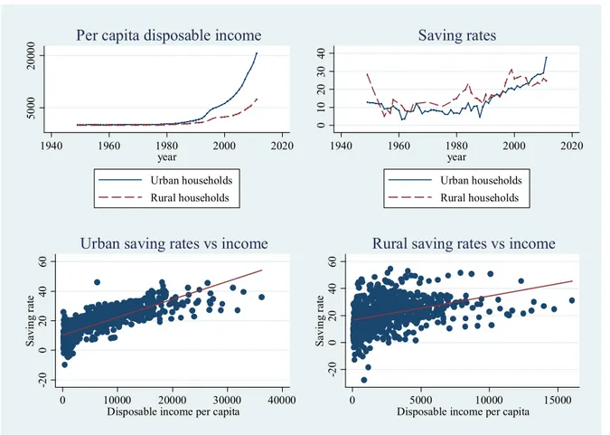
Overall, household saving increased during the last six decades (Table 2). Both urban and rural saving rates exhibit a positive relationship with disposable income (Figure 2), consistent
4 Source: the National Bureau of Statistics of China.
5 The temporary decline in urban worker share at the end of the 1990s may be caused by the slowdown in
economic growth after the Asian crisis, when migrant workers from the rural areas returned home.
with the standard theories on household saving. However, a comparison of urban and rural saving rates reveals a contradiction to the above observation. In spite of an average disposable income two to three times the rural level, urban households saved a smaller portion of their income than did rural households most of the time (Table 2 and Figure 2). Urban households’ more stable income and lower consumption of self-produced goods and services could be factors behind the relatively low urban saving rates, but more prevalent conspicuous consumption in urban areas could be another factor.
Figure 2 – Disposable Income and Saving
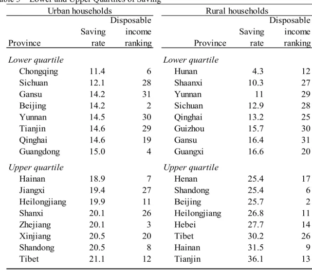
A casual cross-province comparison of consumption and saving patterns also seems to support Veblen’s theory. Coastal provinces exhibit lower saving rates consistently, especially in the South and Southeast, which tend to be more open internationally and attract more migrant workers. For example, in 2011, retail sales of consumption goods as percentages of household disposable income were 80% in Shanghai, 72% in Guangdong, and 67% in Fujian, much higher than those in such inland provinces as Jiangxi (44%), Hunan (55%), and Guizhou (31%). While disposable income seems to play a predominant role in rural saving, there are clearly other factors at play in the ranking of urban saving (Table 3). The eight provinces with the lowest urban saving rates include three of the four metropolises (Chongqing, Beijing, and Tianjin) and Guangdong, a province next to Hong Kong with the most and earliest national economic special zones and the longest history of openness, in spite of their high rankings in disposable income (except for Tianjin). In contrast, most of the eight provinces with the highest urban saving rates are inland provinces and none of them is a metropolis. The next two sections will present a formal model that identifies the individual effects of different determinants of household saving using provincial data.
50 00 20 00 0 1940 1960 1980 2000 2020 year Urban households Rural households
Per capita disposable income
0 10 20 30 40 1940 1960 1980 2000 2020 year Urban households Rural households Saving rates -2 0 0 20 40 60 Sa vi ng ra te 0 10000 20000 30000 40000
Disposable income per capita
Urban saving rates vs income
-2 0 0 20 40 60 Sa vi ng ra te 0 5000 10000 15000
Disposable income per capita
Table 3 – Lower and Upper Quartiles of Saving
Province Saving rate
Disposable income
ranking Province Saving rate
Disposable income ranking
Lower quartile Lower quartile
Chongqing 11.4 6 Hunan 4.3 12 Sichuan 12.1 28 Shaanxi 10.3 27 Gansu 14.2 31 Yunnan 11 29 Beijing 14.2 2 Sichuan 12.9 28 Yunnan 14.5 30 Qinghai 13.2 25 Tianjin 14.6 29 Guizhou 15.7 30 Qinghai 14.6 19 Gansu 16.4 31 Guangdong 15.0 4 Guangxi 16.6 20
Upper quartile Upper quartile
Hainan 18.9 7 Henan 25.4 17 Jiangxi 19.4 27 Shandong 25.4 6 Heilongjiang 19.9 11 Beijing 25.7 2 Shanxi 20.1 26 Heilongjiang 26.8 11 Zhejiang 20.1 3 Hebei 27.7 14 Xinjiang 20.5 20 Tibet 30.2 26 Shandong 20.5 8 Hainan 31.5 9 Tibet 21.1 12 Tianjin 36.1 13
Urban households Rural households
3. Methodology
Because of the panel nature of the data, the following model is considered.
= + , + + + +
In the equation, sit represents saving rate for province i in year t; β0, β1, and the vector β2
are parameters. The lagged saving rate is included as an explanatory variable because of possible inertia in consumption and saving behavior in the short term. X is a vector of explanatory variables. αi accounts for all time-invariant and province specific factors, such as
local cultures affecting consumption and saving; the linear time trend t accounts for common time effects, which are time-varying but common to all panels, such as interest rate and other macroeconomic factors that affect the whole economy. εit is the idiosyncratic disturbance term.
Because the data consists of relatively large numbers of panels, specification of heterogeneous time trends across provinces is not considered. However, heterogeneity in coefficients across urban and rural households is allowed by running separate regressions for the two samples.
The following is a list of the variables included in X. The data source is China Data Online, unless otherwise specified. All flow variables are logarized, including per capita disposable income, government social spending as defined as follows, and those in (5) and (6) in the following list.
(1) Per capita disposable income and its growth. According to the permanent income theory of saving, they should have positive effects on saving if the increase in income is viewed as temporary income.
(2) Old (65 years and older) and young (14 years and younger) dependency ratios. Data is available from 1990 onwards and is obtained from the website of the National Bureau of Statistics of China and its various printed editions of China Population Statistics Yearbooks. Since the sample sizes of the censuses, and hence the dependency ratio data, are drastically different in years 2000, 2005, and 2010 from those in the rest of the years, data for these 3 years are linearly interpolated. According to the life cycle theory, the middle-aged save the most; thus, the age dependency ratios should have negative effects on saving. However, the effects may be muffled if the middle-aged are keen on saving for their children’s future education and are burdened by hikes in education and housing cost, and the old are frugal due to desires to leave bequest to their children and concerns about increased longevity.
(3) Share of urban workers in state-owned enterprises and per capita government spending on culture, education, science, and healthcare (government social spending hereafter). Jobs in state-owned enterprises are viewed as more stable than in private enterprises, although to a lesser extent after privatization of state-owned enterprises started. Note that the share of workers in state-owned enterprises is not considered for rural household saving. Government social spending is considered since it may reduce households’ precautionary saving. These two variables should have negative effects on saving. (4) Share of workers in urban areas as a proxy for the urbanization ratio. It is expected to
have negative effects on both urban and rural saving. A higher urbanization ratio means households are more likely to live in larger communities and population mobility may also be higher. As a result, households are expected to engage in more conspicuous consumption and have lower saving rates. A higher urbanization level also means a higher portion of the rural areas are close to cities, and rural households presumably have more personal connections with urban households. As a result, rural households are also more likely to be exposed to transient observers and influenced by urban cultures. Note that this variable does not represent the differences between urban and rural households in such factors as income uncertainty, since the two samples will be estimated separately.
(5) Passenger traffic to population ratio, per capita business volume of postal communications and telecommunications (communication volume hereafter), and per capita number of telephone units. These variables are not only directly and indirectly associated with the degree of population mobility, they also reflect the intensity of intra- and inter-community interactions. Higher population mobility exerts a negative effect on saving, according to Veblen’s theory. The more intense the interactions are, the more likely a community will undergo cultural changes. The data source used to calculate these ratios is the website and the printed publications of the National Bureau of Statistics of China. Due to a high correlation coefficient (0.97) between per capita communication volume and per capita telephone units, these two variables are included in the regressions separately.7
(6) Variables representing international openness, including per capita foreign direct investment inflows and per capita international trade volume (sum of exports and imports). These two variables measure economic openness and personal contact with
cultures from abroad directly and indirectly. To be consistent with other variables, these variables are recalibrated to measures in Chinese yuan using annual exchange rates from FRED Economic Data, maintained by the Federal Reserve Bank of St. Louis. They should also have negative effects on saving based on previous reasoning. Since the correlation coefficient between them is high (0.85), they are also included in the regressions separately.
Per capita income growth was rising for both urban and rural households from the end of the 1990s to the end of the data period in this study. All other variables exhibited clear upward trends since 1990, except for the young dependency ratio and the share of urban workers in state-owned enterprises, both of which trended downward sharply. All variables are available for all 31 provinces for at least some periods, but the maximum length of over half of the variables is 21-23 years. As a result, the number of panels is considerably greater than the number of periods. Also note that since data availability varies for different variables, the sample size differs slightly when different covariates are included.
The Wooldridge test for serial correlation (Drukker, 2003) rejected the null of no auto-correlation in the idiosyncratic errors. The modified Wald test also detected the presence of group heteroskedasticity. As a result, robust standard errors will be used in all regressions. Cross-sectional dependence is also detected using the Pesaran’s test (De Hoyos & Sarafidis, 2006); thus, the within estimator may be biased, according to Driscoll and Kraay (1998), and regressions with the Driscoll-Kraay standard errors will also be run as an alternative.
The dynamic specification may introduce bias to the fixed effect estimator due to correlation between the lagged saving rate si,t-1 and the error term εit. This problem is magnified
when the number of time periods is short relative to the number of panels, which is the case here. While the number of panels is 31, the panel length is only between 17 and 21, depending on which variables are included in the regressions. Thus, in addition to the fixed effect estimator, regressions are also run using the Arellano-Bond estimator as a better alternative, which corrects for this problem. The Sargan test of over-identifying restrictions failed to reject the joint validity of the instruments at the 1% level in two cases and at least at the 5% level in all other cases, even though heteroskedasticity may cause over-rejection of the test. The Arellano-Bond test results of autocorrelation in first-differenced errors are all satisfactory; that is, there is first order serial correlation in the disturbances, but not the second order.
4. Results
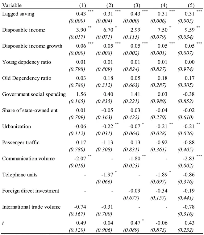
Estimation results are presented in the tables in the Appendix. Table 1 shows the results for urban households using the within estimator. Lagged saving rate, disposable income and its growth are all positive and significant in most cases, as expected. Both young and old dependency ratios are insignificant, probably due to the reasons mentioned in the previous section. In addition, the relatively high correlation between the young dependency ratio and income per capita (correlation coefficients are -0.71 and -0.79 for urban and rural households respectively) may also skew the results.
The coefficients for government social spending and the share of state owned enterprises are not significant, and the signs are inconsistent or not as expected. However, estimations for the variables representing urbanization and population mobility are almost all negative, and are significant across the regressions, except for passenger traffic.
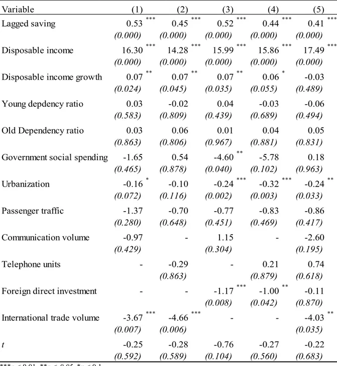
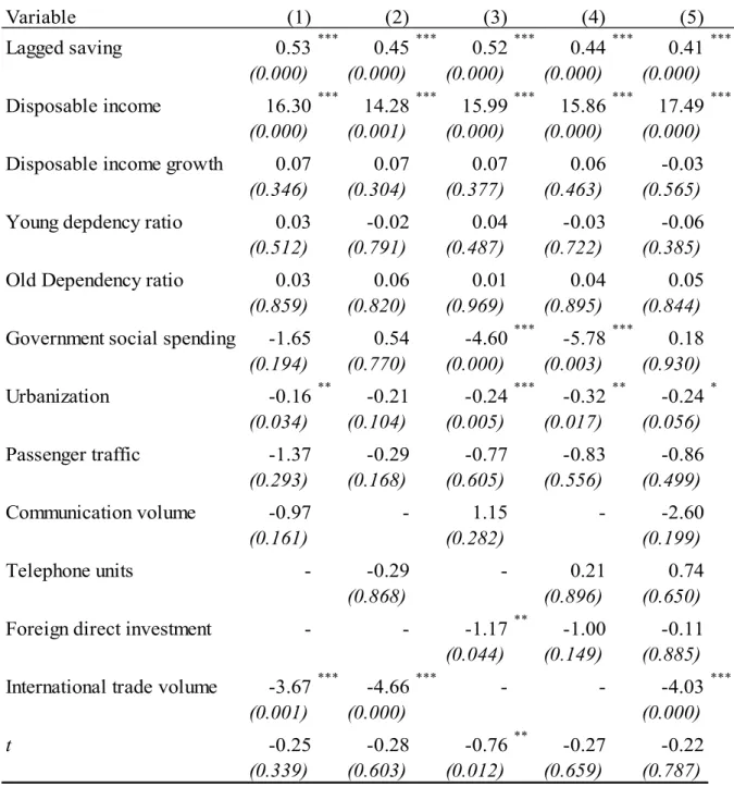
The results for rural households using the within estimator are generally similar (Table 2). However, the income elasticity of saving, indicated by the coefficient of disposable income, is much higher for rural households, probably due to their more cautious attitude towards increased income. That is, increased income is more likely to be treated as temporary income
by rural households. Unlike the regressions for urban households, the parameter for government social spending is negative and significant in one case for rural households. In addition, the coefficient for communication volume is no longer significant; however, those for the variables representing international openness (foreign direct investment and international trade) are both highly significant.
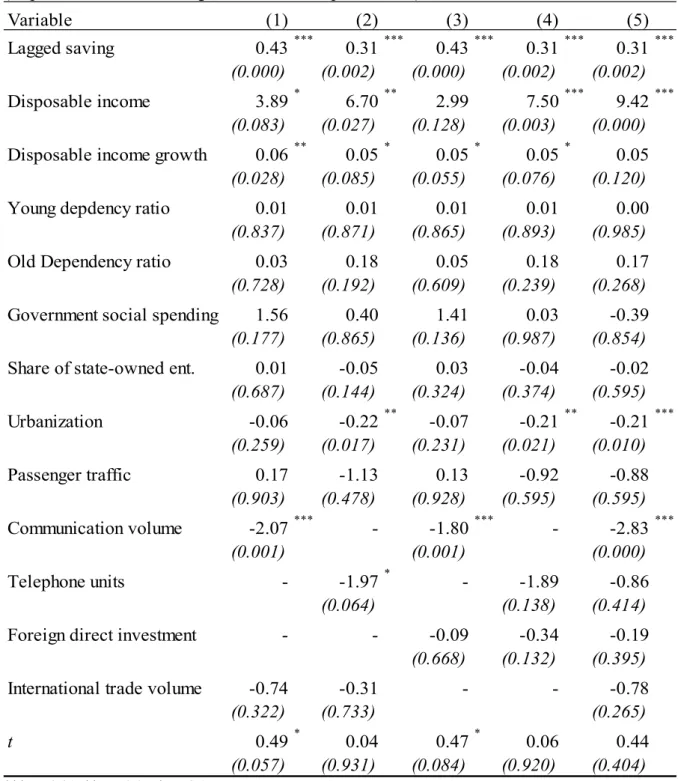
Since the data exhibits cross-sectional dependence, estimations with the within estimator are also obtained using a procedure written by Hoechle (2007) that adopts the Driscoll-Kraay standard errors. The results are reported in Tables 3 and 4. The estimated coefficients are similar in general, but the p-values are different for some variables. The biggest change is that disposable income growth is now insignificant for rural households. However, the variables affecting precautionary saving and conspicuous consumption (the variables in (3) – (6) in the previous section) are still negative in general. As in previous regressions, the urbanization ratio is again significant in most regressions. Government social spending, communication volume, per capita telephone units, foreign direct investment, and international trade are also significant in some regressions.
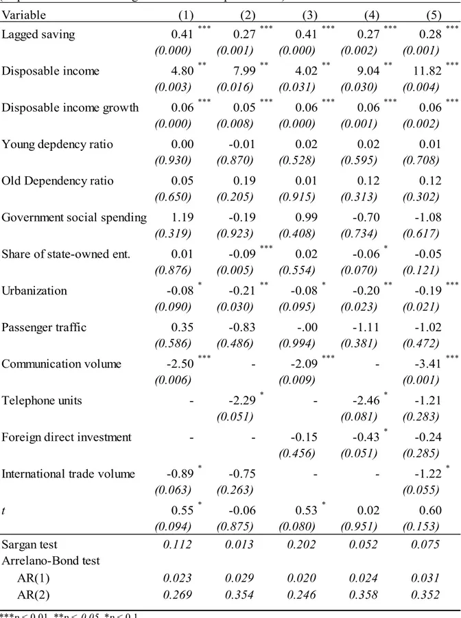
The estimation results using the Arellano-Bond robust estimator are reported in Tables 5 and 6 in the Appendix, along with the results of the Sargan test and the Arellano-Bond test. The results are largely the same as with the within estimator. For the variables in (3) to (6) in the variable list, the coefficients are generally negative, as expected, but the p-values for the vast majority of them are lower. Thus, there are more significant estimations for the urban household sample. The coefficients for urbanization and communication volume are consistently significant, and the share of state-owned enterprises, per capita telephone units, foreign direct investment, and international trade are also significant in about half of the regressions.
As a robustness check, regressions are also run with no time trend, a quadratic trend, and time dummies in lieu of a linear trend. Both components of the quadratic trend are insignificant in all regressions except for one, but the hypothesis that all time dummies are zeros is strongly rejected. The results are not drastically different from previous regressions (see Table 7 for some of the results using the Arellano-Bond estimator). Disposable income and its growth continue to have positive and significant estimates. Estimations for the age dependency ratios are still largely insignificant. The parameters for the variables representing urbanization, population mobility, and international openness continue to be negative and significant in many of the regressions.
In summary, the estimation results are robust using alternative estimators, explanatory variables, and specifications of the common time effects. Of all the explanatory variables, only two variables, disposable income and its growth, are estimated to have positive effects on household saving without ambiguity. These variables trended up in the past several decades, which were major factors for past increase in household saving. However, as economic growth slows down inevitably, the support of higher saving rates from disposable income increase is bound to fade in the future.
Little evidence is found for the life cycle theory through the results on the age dependency ratios. However, all other variables in the model are estimated to have negative effects on saving to various degrees of consistency. The estimations for government social spending (for rural households mainly) and the share of workers in state-owned enterprises (for urban households) suggest weak evidence of previous increase in precautionary saving. As households are weaned off government provided education and healthcare, precautionary saving may continue to increase, but only to a limited extent given that social welfare measures in rural areas are improving and the provincial mean share of state-owned enterprises already dropped to 14.4% in 2011.
Meanwhile, the variables that would enhance conspicuous consumption will most likely trend up in the future, including the urbanization ratio, the variables representing population mobility and interactions (passenger traffic, communication volume, telephone units) and international openness (foreign direct investment and international trade volume), further putting downward pressure on saving. Urbanization will likely accelerate as the government is considering it a priority to aid future economic transformation. Population mobility will continue to increase with the relaxation of restrictions on labor mobility. Status goods will become more readily available as international trade expands. Cultural influences from the rest of the world will permeate further and individuals’ life styles will continue to transform as international openness deepens. Together, these factors can outweigh the positive effect of higher income, and the current high household saving may not persist.
5. Final remarks
In addition to conventional theories, this paper considers the rapid cultural and social changes that are happening in China and incorporates non-conventional theories on consumption and saving that help explain China’s household saving patterns. Among the conventional explanatory variables, the paper finds that per capita disposable income and its growth contribute to higher household saving, consistent with the permanent income theory. The young and old dependency ratios are generally insignificant with few exceptions, and the signs are not consistent. This insignificance may be caused by the custom of bequeathing, increased longevity, altruistic saving for children’s education, increase in education and housing cost, and correlation between the young age dependency ratio and per-capita disposable income.
The paper’s unique contribution to the literature is the exploration of the possible presence of conspicuous consumption in China and its effect on household saving. Expanding from Veblen’s theory, it finds evidence that urbanization, increased population mobility, and a greater degree of international openness all depress household saving, likely through higher conspicuous consumption. The list of explanatory factors is further broadened from the perspective of precautionary saving, and there is evidence that while the decline in state ownership prompted urban households to save more, increased government spending on education and healthcare may have the opposite effect in rural areas.
Observations of conspicuous consumption as a potential contributing factor to declining household saving are certainly not confined to this research or to the Chinese economy, as reviewed in the first section of this paper. As international openness coupled with rapid economic development often leads to cultural shifts, swift urbanization, and increased population mobility, the findings on Chinese household saving could also shed light on household saving trends in other developing and emerging countries which are following the footsteps of China, such as India, Vietnam, and Cambodia.
As an important component of national saving, household saving is a critical source for financing investment, especially when the government and businesses engage in excessive borrowing, as China is currently experiencing, and many other emerging economies experienced in the past, such as those in predicament during the East Asian financial crisis. If excess status consumption becomes widespread and the competitive nature of conspicuous consumption is unleashed, the resulting decline in household saving can be self-reinforcing. The implications can be particularly grave for developing and emerging economies with their growth relying more on investment, but their ability to borrow from the international market far more limited than developed economies.
The policy implications of the findings in association with changing patterns of households saving can be far-reaching, ranging from taxation on luxury goods (see Bagwell & Bernheim, 1996), to evaluation of financing sources of investment, and long term growth strategies for
developing and emerging economies. The choice of policy regime leading to or away from a more egalitarian society also matters to saving and economic growth to the extent that wealth distribution influences the drive for conspicuous consumption, although the overall link between economic inequality and household saving is still much debatable, as Corneo and Jeanne (2001) and Roychowdhury (2017) showed.
Future avenues of further investigation may include incorporating provincial level data that reflects household assets, life expectancy, corporate saving, housing price indexes (ideally differentiating between the rural and urban housing markets), and other factors that may affect household saving. Moreover, it will be worthwhile to confirm the findings and further understand this issue using household level data. As empirical work on conspicuous consumption is still relatively rare and the topic remains inadequately researched, similar studies can be extended to economies that are also undergoing rapid changes economically and culturally.
Appendix
Table 1 – Urban Households: the Within Estimator with Linear Time Trend (Dependent variable: saving rate. P-values in parentheses)
Variable (1) (2) (3) (4) (5) Lagged saving 0.43 *** 0.31 *** 0.43 *** 0.31 *** 0.31 ***
(0.000) (0.004) (0.000) (0.006) (0.005) Disposable income 3.90 ** 6.70 * 2.99 7.50 * 9.59 **
(0.017) (0.071) (0.115) (0.079) (0.034) Disposable income growth 0.06 *** 0.05 *** 0.05 *** 0.05 *** 0.05 ***
(0.000) (0.008) (0.002) (0.001) (0.007) Young depdency ratio 0.01 0.01 0.01 0.01 0.00
(0.798) (0.809) (0.824) (0.827) (0.974) Old Dependency ratio 0.03 0.18 0.05 0.18 0.17
(0.780) (0.312) (0.663) (0.287) (0.305) Government social spending 1.56 0.40 1.41 0.03 -0.38
(0.165) (0.835) (0.221) (0.989) (0.852) Share of state-owned ent. 0.01 -0.05 0.03 -0.04 -0.02
(0.709) (0.163) (0.422) (0.279) (0.610) Urbanization -0.06 -0.22** -0.07* -0.21** -0.21 ** (0.112) (0.031) (0.064) (0.028) (0.026) Passenger traffic 0.17 -1.13 0.13 -0.92 -0.88 (0.780) (0.308) (0.831) (0.361) (0.405) Communication volume -2.07** - -1.80** - -2.83 *** (0.018) (0.023) (0.002) Telephone units - -1.97* - -1.89* -0.86 (0.066) (0.097) (0.376) Foreign direct investment - - -0.09 -0.34 -0.19
(0.677) (0.157) (0.441) International trade volume -0.74 -0.31 - - -0.78
(0.167) (0.700) (0.316) t 0.49 0.04 0.47 * -0.06 0.43
(0.120) (0.906) (0.089) (0.873) (0.252)
Table 2 – Rural Households: The Within Estimator with Linear Time Trend (Dependent variable: saving rate. P-values in parentheses)
Variable (1) (2) (3) (4) (5)
Lagged saving 0.53*** 0.45 *** 0.52*** 0.44 *** 0.41 ***
(0.000) (0.000) (0.000) (0.000) (0.000) Disposable income 16.30 *** 14.28 *** 15.99*** 15.86 *** 17.49 ***
(0.000) (0.000) (0.000) (0.000) (0.000) Disposable income growth 0.07** 0.07 ** 0.07** 0.06 * -0.03
(0.024) (0.045) (0.035) (0.055) (0.489)
Young depdency ratio 0.03 -0.02 0.04 -0.03 -0.06
(0.583) (0.809) (0.439) (0.689) (0.494)
Old Dependency ratio 0.03 0.06 0.01 0.04 0.05
(0.863) (0.806) (0.967) (0.881) (0.831)
Government social spending -1.65 0.54 -4.60** -5.78 0.18
(0.465) (0.878) (0.040) (0.102) (0.963) Urbanization -0.16 * -0.10 -0.24*** -0.32 *** -0.24** (0.072) (0.116) (0.002) (0.003) (0.033) Passenger traffic -1.37 -0.70 -0.77 -0.83 -0.86 (0.280) (0.648) (0.451) (0.469) (0.417) Communication volume -0.97 - 1.15 - -2.60 (0.429) (0.304) (0.195) Telephone units - -0.29 - 0.21 0.74 (0.863) (0.879) (0.618)
Foreign direct investment - - -1.17*** -1.00 ** -0.11
(0.008) (0.042) (0.870) International trade volume -3.67 *** -4.66*** - - -4.03**
(0.007) (0.006) (0.035)
t -0.25 -0.28 -0.76 -0.27 -0.22
(0.592) (0.589) (0.104) (0.560) (0.683)
Table 3 – Urban Households: The Within Estimator with Driscoll and Kraay Standard Errors (Dependent variable: saving rate. P-values in parentheses)
Variable (1) (2) (3) (4) (5)
Lagged saving 0.43*** 0.31 *** 0.43*** 0.31 *** 0.31 ***
(0.000) (0.002) (0.000) (0.002) (0.002)
Disposable income 3.89* 6.70 ** 2.99 7.50 *** 9.42 ***
(0.083) (0.027) (0.128) (0.003) (0.000) Disposable income growth 0.06** 0.05 * 0.05* 0.05 * 0.05
(0.028) (0.085) (0.055) (0.076) (0.120)
Young depdency ratio 0.01 0.01 0.01 0.01 0.00
(0.837) (0.871) (0.865) (0.893) (0.985)
Old Dependency ratio 0.03 0.18 0.05 0.18 0.17
(0.728) (0.192) (0.609) (0.239) (0.268)
Government social spending 1.56 0.40 1.41 0.03 -0.39
(0.177) (0.865) (0.136) (0.987) (0.854)
Share of state-owned ent. 0.01 -0.05 0.03 -0.04 -0.02
(0.687) (0.144) (0.324) (0.374) (0.595) Urbanization -0.06 -0.22** -0.07 -0.21 ** -0.21*** (0.259) (0.017) (0.231) (0.021) (0.010) Passenger traffic 0.17 -1.13 0.13 -0.92 -0.88 (0.903) (0.478) (0.928) (0.595) (0.595) Communication volume -2.07 *** - -1.80*** - -2.83 *** (0.001) (0.001) (0.000) Telephone units - -1.97* - -1.89 -0.86 (0.064) (0.138) (0.414)
Foreign direct investment - - -0.09 -0.34 -0.19
(0.668) (0.132) (0.395)
International trade volume -0.74 -0.31 - - -0.78
(0.322) (0.733) (0.265)
t 0.49* 0.04 0.47* 0.06 0.44
(0.057) (0.931) (0.084) (0.920) (0.404)
Table 4 – Rural Households: The Within Estimator with Driscoll and Kraay Standard Errors (Dependent variable: saving rate. P-values in parentheses)
Variable (1) (2) (3) (4) (5)
Lagged saving 0.53*** 0.45 *** 0.52*** 0.44 *** 0.41 ***
(0.000) (0.000) (0.000) (0.000) (0.000) Disposable income 16.30 *** 14.28 *** 15.99*** 15.86 *** 17.49 ***
(0.000) (0.001) (0.000) (0.000) (0.000)
Disposable income growth 0.07 0.07 0.07 0.06 -0.03
(0.346) (0.304) (0.377) (0.463) (0.565)
Young depdency ratio 0.03 -0.02 0.04 -0.03 -0.06
(0.512) (0.791) (0.487) (0.722) (0.385)
Old Dependency ratio 0.03 0.06 0.01 0.04 0.05
(0.859) (0.820) (0.969) (0.895) (0.844) Government social spending -1.65 0.54 -4.60*** -5.78 *** 0.18
(0.194) (0.770) (0.000) (0.003) (0.930) Urbanization -0.16 ** -0.21 -0.24*** -0.32 ** -0.24* (0.034) (0.104) (0.005) (0.017) (0.056) Passenger traffic -1.37 -0.29 -0.77 -0.83 -0.86 (0.293) (0.168) (0.605) (0.556) (0.499) Communication volume -0.97 - 1.15 - -2.60 (0.161) (0.282) (0.199) Telephone units - -0.29 - 0.21 0.74 (0.868) (0.896) (0.650)
Foreign direct investment - - -1.17** -1.00 -0.11
(0.044) (0.149) (0.885) International trade volume -3.67 *** -4.66*** - - -4.03***
(0.001) (0.000) (0.000)
t -0.25 -0.28 -0.76** -0.27 -0.22
(0.339) (0.603) (0.012) (0.659) (0.787)
Table 5 – Urban Households: Arellano-Bond Estimator with Time Trend (Dependent variable: saving rate. P-values in parentheses)
Variable (1) (2) (3) (4) (5)
Lagged saving 0.41 *** 0.27 *** 0.41*** 0.27 *** 0.28 ***
(0.000) (0.001) (0.000) (0.002) (0.001)
Disposable income 4.80 ** 7.99 ** 4.02** 9.04 ** 11.82 ***
(0.003) (0.016) (0.031) (0.030) (0.004) Disposable income growth 0.06 *** 0.05 *** 0.06*** 0.06 *** 0.06 ***
(0.000) (0.008) (0.000) (0.001) (0.002)
Young depdency ratio 0.00 -0.01 0.02 0.02 0.01
(0.930) (0.870) (0.528) (0.595) (0.708)
Old Dependency ratio 0.05 0.19 0.01 0.12 0.12
(0.650) (0.205) (0.915) (0.313) (0.302)
Government social spending 1.19 -0.19 0.99 -0.70 -1.08
(0.319) (0.923) (0.408) (0.734) (0.617) Share of state-owned ent. 0.01 -0.09*** 0.02 -0.06 * -0.05
(0.876) (0.005) (0.554) (0.070) (0.121) Urbanization -0.08 * -0.21** -0.08 * -0.20 ** -0.19*** (0.090) (0.030) (0.095) (0.023) (0.021) Passenger traffic 0.35 -0.83 -.00 -1.11 -1.02 (0.586) (0.486) (0.994) (0.381) (0.472) Communication volume -2.50 *** - -2.09 *** - -3.41 *** (0.006) (0.009) (0.001) Telephone units - -2.29* - -2.46 * -1.21 (0.051) (0.081) (0.283)
Foreign direct investment - - -0.15 -0.43 * -0.24
(0.456) (0.051) (0.285)
International trade volume -0.89 * -0.75 - - -1.22*
(0.063) (0.263) (0.055) t 0.55 * -0.06 0.53* 0.02 0.60 (0.094) (0.875) (0.080) (0.951) (0.153) Sargan test 0.112 0.013 0.202 0.052 0.075 Arrelano-Bond test AR(1) 0.023 0.029 0.020 0.024 0.031 AR(2) 0.269 0.354 0.246 0.358 0.352 ***p < 0.01, **p < 0.05, *p < 0.1
Table 6. Rural Households: Arellano-Bond Estimator with Time Trend (Dependent variable: saving rate. P-values in parentheses)
Variable (1) (2) (3) (4) (5) Lagged saving 0.52 *** 0.45 *** 0.48*** 0.41 *** 0.44 ***
(0.000) (0.000) (0.000) (0.000) (0.000) Disposable income 16.81 *** 14.30 *** 15.77 *** 15.42 *** 17.38 ***
(0.000) (0.000) (0.000) (0.000) (0.000) Disposable income growth 0.07 ** 0.07 ** 0.04 0.03 0.06
(0.027) (0.025) (0.399) (0.493) (0.133) Young depdency ratio 0.02 -0.03 0.04 -0.02 -0.01
(0.710) (0.697) (0.341) (0.786) (0.852) Old Dependency ratio 0.02 0.03 -0.08 -0.07 -0.09
(0.893) (0.892) (0.613) (0.731) (0.662) Government social spending -1.58 1.03 -3.98 * -4.99 -0.50
(0.508) (0.788) (0.072) (0.203) (0.896) Urbanization -0.16* -0.18 -0.23 *** -0.27*** -0.18* (0.066) (0.136) (0.001) (0.002) (0.061) Passenger traffic -1.75 -0.26 -1.66 -1.27 -0.42 (0.181) (0.878) (0.250) (0.422) (0.802) Communication volume -1.47 - 1.11 - -3.39 (0.274) (0.369) (0.161) Telephone units - -1.14 - -0.22 -0.25 (0.534) (0.874) (0.881) Foreign direct investment - - -1.07 * -0.87 -0.32
(0.081) (0.207) (0.703) International trade volume -4.10*** -5.17 *** - - -5.09***
(0.001) (0.001) (0.002) t -0.08 -0.05 -0.75 -0.15 0.76 (0.877) (0.934) (0.117) (0.763) (0.232) Sargan test 0.023 0.016 0.105 0.073 0.054 Arrelano-Bond test AR(1) 0.000 0.001 0.000 0.001 0.001 AR(2) 0.979 0.982 0.953 0.830 0.829 ***p < 0.01, **p < 0.05, *p < 0.1
Table 7 – Alternative specifications of common time effects with the Arellano-Bond estimator (Dependent variable: saving rate. P-values in parentheses)
Variable Urban Rural Urban Rural Urban Rural
Lagged saving 0.41 *** 0.52 *** 0.40 *** 0.52 *** 0.47 *** 0.43 *** (0.000) (0.000) (0.000) (0.000) (0.000) (0.000) Disposable income 5.03 *** 16.64 *** 7.23 ** 16.28 *** 7.10 ** 25.54 *** (0.003) (0.000) (0.023) (0.000) (0.046) (0.000) 0.06 *** 0.07 * 0.06 *** 0.07 ** 0.20 *** 0.24 *** (0.000) (0.060) (0.001) (0.014) (0.000) (0.000) 0.02 0.02 0.01 0.02 -0.04 0.12 * (0.610) (0.684) (0.844) (0.734) (0.225) (0.085) 0.05 0.03 0.05 0.01 0.03 -0.30 * (0.628) (0.885) (0.663) (0.969) (0.762) (0.076) 2.46 *** -2.17 -0.40 -1.02 -0.70 -0.86 (0.006) (0.212) (0.854) (0.697) (0.747) (0.731) -0.04 - 0.00 - 0.02 -(0.231) (0.986) (0.675) Urbanization -0.12** -0.14 * -0.08 * -0.16 * -.00 -0.15 ** (0.015) (0.075) (0.079) (0.079) (0.999) (0.034) Passenger traffic 0.17 -1.82 0.23 -1.69 0.48 -1.65 ** (0.782) (0.154) (0.713) (0.230) (0.318) (0.049) -1.73*** -1.34 -1.97 *** -1.80 -1.36** 1.14 (0.003) (0.167) (0.009) (0.332) (0.044) (0.445) -0.91** -4.11 *** -1.00 ** -4.08 *** -0.12 -0.91 (0.046) (0.001) (0.031) (0.004) (0.763) (0.342) t - - -0.02 0.10 - -(0.954) (0.912) t2 - - 0.02 -0.01 - -(0.231) (0.710)
No trend Quadratic trend Time dummies
Communication volume International trade volume Disposable income growth Young depdency ratio Old Dependency ratio Government social spending Share of state-owned enterprises ***p < 0.01, **p < 0.05, *p < 0.1
References
1. Bagwell, L. S., & Bernheim, B. D. (1996). Veblen effects in a theory of conspicuous consumption. American Economic Review, 86(3), 349–373.
2. Bourdieu, P. (1984). Distinction : A Social Critique of The Judgement of Taste. London: Routledge.
3. Chamon, M., Liu, K., & Prasad, E. (2013). Income Uncertainty and Household Savings in China. Journal of Development Economics, 105(November), 164–77.
4. Chen, X. (2017a). Globalization and Household Saving: Is There a Link? Applied Economics, 49(29), 2797–2816.
5. Chen, X. (2017b). Why Do Migrant Households Consume So Little? Asian Development Bank Institute Working Paper, 727.
6. Cheung, D., & Padieu, Y. (2015). Heterogeneity of the Effects of Health Insurance on Household Savings: Evidence from Rural China. World Development, 66(February), 84– 103.
7. Corneo, G., & Jeanne, O. (2001). Status, the Distribution of Wealth, and Growth. The Scandinavian Journal of Economics, 103(2), 283–293.
8. Cristadoro, R., & Marconi, D. (2012). Household Savings in China. Journal of Chinese Economic and Business Studies, 10(3), 275–299.
9. Curtis, C. C., Lugauer, S., & Mark, N. C. (2015). Demographic Patterns and Household Saving in China. American Economic Journal: Macroeconomics, 7(2), 58–94.
10. Danzer, A. M., Dietz, B., Gatskova, K., & Schmillen, A. (2014). Showing Off to the New Neighbors? Income, Socioeconomic Status and Consumption Patterns of Internal Migrants. Journal of Comparative Economics, 42(1), 230–245.
11. De Hoyos, R. E., & Sarafidis, V. (2006). Testing for cross–sectional dependence in panel– data models. Stata Journal, 6(4), 482–496.
12. Doctoroff, T. (2012, May 18). What the Chinese Want. The Wall Street Journal. Retrieved from http://online.wsj.com/.
13. Dreher, A. (2006). Does Globalization Affect Growth? Evidence from a new Index of Globalization. Applied Economics, 38(10), 1091–1110.
14. Dreher, A., Gaston, N., & Martens, P. (2008). Measuring Globalisation – Gauging its Consequences. New York: Springer.
15. Driscoll, J. C., & Kraay, A. C. (1998). Consistent covariance matrix estimation with spatially dependent panel data. Review of Economics and Statistics, 80(4), 549–560. 16. Drukker, D. M. (2003). Testing for serial correlation in linear panel-data models. The Stata
Journal, 3(2), 168–177.
17. Dutt, A. K. (2001). Consumption, Happiness, and Religion. In Crossing the mainstream: Ethical and methodological issues in economics (pp. 133–69). Notre Dame: University of Notre Dame Press.
18. Feng, J., He, L., & Sato, H. (2011). Public Pension and Household Saving: Evidence from Urban China. Journal of Comparative Economics, 39(4), 470–485.
19. Goldstein, M. (2014, February 11). U.S. Targets Buyers of China-Bound Luxury Cars. New York Times.
20. Guarneros, V., Narváezy, A., & Vilar, M. (2001). Consumption in a rapidly changing society: the Mexican case. In Youth, sustainable consumption patterns and life styles by UNESCO and UNEP (pp. 141–66). UNESCO and UNEP.
21. Guo, C. (2012, August 9). High Schooler’s Kidney for “Apples” Case Opens in Chenzhou. Sanxiang City Post (三湘都市报). Retrieved from http://sxdsb.voc.com.cn.
22. Heatley, C. (2011, December 12). English Butlers Wanted For Super-Rich Clients in China, Russia. Bloomberg News.
23. Heffetz, O. (2011). A Test of Conspicuous Consumption: Visibility and Income Elasticities. Review of Economics and Statistics, 93(4), 1101–1117.
24. Hoechle, D. (2007). Robust standard errors for panel regressions with cross-sectional dependence. Stata Journal, 7(3), 281–312.
25. Horioka, C. Y., & Wan, J. (2007). The Determinants of Household Saving in China: A Dynamic Panel Analysis of Provincial Data. Journal of Money, Credit and Banking, 39(8), 2077–2096.
26. Kim, J.-O., Forsythe, S., Gu, Q., & Moon, S. J. (2002). Cross-cultural consumer values, needs and purchase behavior. Journal of Consumer Marketing, 19(6), 481–502.
27. Kraay, A. (2000). Household Saving in China. World Bank Economic Review, 14(3), 545– 570.
28. Li, S., Whalley, J., & Zhao, X. (2013). Housing Price and Household Savings Rates: Evidence from China. Journal of Chinese Economic and Business Studies, 11(3), 197–217. 29. Lim, L. (2012, January 11). China Targets Entertainment TV In Cultural Purge. National
Public Radio. Retrieved from www.npr.org.
30. Liu, S., & Hu, A. (2013). Household Saving in China: The Keynesian Hypothesis, Life-Cycle Hypothesis, and Precautionary Saving Theory. Developing Economies, 51(4), 360– 87.
31. Roychowdhury, P. (2017). Visible Inequality, Status Competition and Conspicuous Consumption: Evidence from India. Oxford Economic Papers, 69(1), 36–54. doi: 10.1093/oep/gpw056.
32. Schor, J. (2007). In Defense of Consumer Critique: Revisiting the Consumption Debates of the Twentieth Century. Annals of the American Academy of Political and Social Science, 611(1), 16–30.
33. Trigg, A. B. (2001). Veblen, Bourdieu, and Conspicuous Consumption. Journal of Economic Issues, 35(1), 99–115.
34. United Nations. (2009). System of national accounts 2008. New York: United Nations. 35. Veblen, T. ([1899] 2007). The theory of the leisure class (Reprint. Edited with an
Introduction and Notes by Martha Banta.). New York: Oxford University Press.
36. Wang, X., & Wen, Y. (2012). Housing Prices and the High Chinese Saving Rate Puzzle. China Economic Review, 23(2), 265–283.
37. Yin, T. (2012). The “Will” to Save in China: The Impact of Bequest Motives on the Saving Behavior of Older Households. Japanese Economy, 39(3), 99–135.
38. Yuan, X., Song, T. H., & Kim, S. Y. (2011). Cultural Influences on Consumer Values, Needs and Consumer Loyalty Behavior: East Asian Culture versus Eastern European Culture. African Journal of Business Management, 5(30), 12184–12196.
39. Zhou, W. (2014). Brothers, Household Financial Markets and Savings Rate in China. Journal of Development Economics, 111(November), 34–47.