Contagio nei principali mercati CDS dopo la
crisi finanziaria globale: un approccio
AR-FIGARCH-cDCC multivariato
di Konstantinos Tsiaras* e Theodore Simos†
Abstract
L’articolo considera correlazioni condizionali time-varying tra i ritorni dei Credit Default Swap (CDS) sovrani per Germania, Francia, Cina e Giappone rispetto agli USA. Utilizziamo un modello cDCC-AR-FIGARCH per identificare potenziali effetti contagio tra mercati nel periodo 2011-2018. I risultati non rigettano l’ipotesi di contagio per le coppie Germania-Francia, Germania-Giappone e Francia-Giappone, mentre non si osserva supporto empirico per l’ipotesi di contagio tra Cina e gli altri paesi.
Parole chiave: contagio finanziario, crisi finanziaria globale, modello
cDCC-AR-FIGARCH, mercato dei CDS sovrani
Classificazione JEL: C58, F30, G01, G15
Contagion in major CDS markets for the post
Global Financial Crisis: A multivariate
AR-FIGARCH-cDCC approach
Abstract
We explore the time-varying conditional correlations of the Sovereing CDS spread returns for Germany, France, China and Japan against USA. We employ a cDCC-AR-FIGARCH model in order to capture potential contagion effects between the markets during the 2011-2018 post global financial crisis. Empirical results do not reject contagion for the country pairs: Germany – France, Germany – Japan and France – Japan while there is little support for contagion among China and the rest of the countries.
Keywords: Financial contagion, Global Financial Crisis,
cDCC-AR-FIGARCH model, Sovereign CDS market
JEL classification: C58, F30, G01, G15
* University of Ioannina, Ioannina, Greece. E-mail: [email protected] † University of Ioannina, Ioannina, Greece. E-mail: [email protected]
1. Introduction
This paper investigates the volatility transmission among major CDS markets, considering the credit risk entailed and how easy can be transferred (Hull 2008). Although the study of integration between derivative markets and financial markets is ubiquitous, there is little work on CDS market integration (Caporale, Pittis and Spagnolo 2006). According to extant research, there are two mechanisms on volatility transmission (Stevens 2008). The first mechanism refers to the common shocks, whilst the second mechanism deals with the spillover effects (Didier, Mauro and Schmuckler 2008). For our study, we use the phenomenon of spillover effects to explain financial contagion. Today, there is still large divergence among economics about what contagion is exactly and how it should be measured and tested empirically. In this paper, we adopt the definition of contagion suggested by Forbes and Rigobon (2002). Theydefined contagion as a significant increase in cross-market linkages after a shock.
The main body of the current literature explores the linkages between CDS markets or between CDS markets with other financial markets, including: Meng, Gwilym and Varas (2009), Lake and Apergis (2009), Schreiber, Muller, Kluppelberg and Wagner (2009), Belke and Gokus (2011), Calice, Chen and Williams (2011), Fonseca and Gottschalk (2012), Koseoglu (2013) and Tokat (2013), among others. Meng, Gwilym and Varas (2009) examine the volatility transmission among the daily 5-year maturity bond, CDS and equity markets for ten large US companies. While they use a multivariate GARCH-BEKK model during 2003-2005, they provide evidence on spillovers. Lake and Apergis (2009) investigate the spillovers among the US and European (German, UK and Greek) 5-year maturity CDS spreads and equity returns in the period 2004-2008. By making use of daily observations, they employ and MVGARCH-M model, finding evidence of spillover effects. Schreiber, Muller, Kluppelberg and Wagner (2009) explore the volatility effects between aggregate CDS premiums, equity returns and implied equity volatility during 2004-2009. They use daily observations of the 5-year maturity CDS iTraxx Europe, Dow Jones Euro Stoxx 50 and Dow Jones VStoxx indexes. By fitting VAR-GARCH models, they show strong evidence of spillovers. Belke and Gokus (2011) examine the volatility transmission among the daily equity prices, CDS premiums and bond yields returns for four large US banks for the period 2006-2009. By employing a BEKK-GARCH model, they capture spillover effects. Calice, Chen &
Williams (2011) investigate the dynamic interactions in the Eurozone1
between 5- and 10-year maturity sovereign CDS premiums and bonds from 2000 to 2010. Using intraday data, they employ a VAR model, pointing out spillovers. Fonseca and Gottschalk (2012) examine the volatility spillovers among CDS premium and equity returns for Australia, Japan, Korea and Hong Kong at firm and index level. To compute the realized volatility they use the TSRV estimator. They use weekly data during 2007-2010 and they show empirical evidence of spillover effects. Koseoglu (2013) investigates the way that ISE100 stock index spills over with 5-year maturity sovereign CDS premiums of Turkey during the period from 2005 to 2012. The data frequency is daily. He uses a VAR-diagonal BEKK model and he finds evidence of spillovers. Tokat (2013) empirically2 investigates the spillover
effects between daily 5-year maturity sovereign CDS values for Brazil and Turkey denominated in USD, iTraxx XO index and CDX index during the period from 2005 to 2011. He employs a full BEKK-GARCH model and he proves empirically the existence of spillovers.
In this paper, we extend the correlation analysis of Forbes and Rigobon (2002) by considering the corrected Dynamic Conditional Correlation Auto Regressive Fractionally Integrated GARCH3 (cDCC-AR-FIGARCH) of
Aielli (2008) that improves the Dynamic Conditional Correlation (DCC-GARCH) model of Engle (2002). Compared to extant empirical research, we take a different perspective by consolidating important elements of financial analysis: long memory, speed of market information and a reformulated driving process of standardized residuals. The main objective is to model financial contagion4 phenomenon (Anderson 2010) among four major
sovereign CDS spread returns (Wei 2008), namely the Germany, France, Japan and China against the USA from 5th October 2011 to 5th February
20185. We consider three dominant world economies (USA, China, Japan)
and the two most important European economies (Germany, France) due to the ongoing European crisis. The data set entails 20-years maturity CDS
1 The countries under investigation European are: Austria, Belgium, France, Greece,
Ireland, Italy, Netherlands, Portugal and Spain.
2 Financial researchers and academics are interested to 5-year maturity CDSs,
investigating the underlying contagion mechanisms in the short-term period.
3 Worthington and Higgs (2003) highlight the importance of multivariate GARCH
models.
4 Missio and Watzka (2011) summarize all the existing different contagion definitions in
the literature and draw up a report of the five most important.
5 Firstly, we defined two periods: one crisis period (2008-2011) and one after-crisis period
(2011-2018). However, we used only the after-crisis period due to autocorrelation and diagnostic tests problems of the crisis period.
premium mid prices6 (Blanco, Brennan and Marsh 2005; Zhu and Yang
2004). We make the hypothesis that the sovereign CDS markets reflect the macroeconomic environment of the countries. The above countries are connected in a macroeconomic level and we expect that the respective sovereign CDS markets will be also connected.
Fig. 1 Actual series of 20-year maturity CDS premium mid prices for all markets.
Notes: Data from Datastream. The lines represent the Sovereign CDS premium mid prices for China, Germany, USA, France and Japan.
Based on our empirical research, several questions arise: (ⅰ) does the dynamic conditional correlation between the CDS markets increase after the recent Global Financial Crisis (GFC) and the beginning of the European Sovereign Dept Crisis (ESDC) 7? (ⅱ) is the dynamic conditional correlation
volatile? (ⅲ) are there evidence of contagion effects?
The paper is organized at follows: Section 2 describes the CDS market framework, followed by an overview of the markets in Section 3. Section 4
6CDS premiums are normally affected by liquidity as many researchers have mentioned,
i.e. Sarig and Warga (1989) and Chen, Lesmond and Wei (2007), among others. The most commonly used are the 5- and 10-year maturity sovereign CDS premiums.
7 The Eurozone Sovereign Debt Crisis of 2009 is also as Aegean Contagion known by
describes the model and the data. Section 5 considers the empirical results, while Section 6 concludes.
2. The CDS market framework
We start this section by providing the CDS definition, the way that CDS market operates and relevant historical data. We define credit default swap (CDS) as a financial swap agreement between two parties: the protection buyer (long position) and the protection seller (short position). The protection buyer pays a periodic fee (CDS premium) to the protection seller. Normally, credit default swap protects the buyer from any future default. However, even a speculator for investment can buy a credit default swap.
Credit default swaps exist since 1994 when J.P. Morgan used them for the first time in the history. In 2007 CDS market developed rapidly. During the period 2007-2010 CDS market became a very large derivative market of a total $62.2 trillion. The main reason for this huge growth was the lack of regulation. Interestingly, by 2012 CDS market fell to $25.6 trillion. In 14th
March 2012, European Union published a new regulation (No 236/2012) on short selling and certain aspects of CDS in the official journal of the European Union. The regulation set up some new restrictions about the short selling of sovereign debt instruments and the taking of sovereign credit default swaps positions. Credit default swaps played an important role in the recent global financial crisis of 2007. They became a leading indicator, reflecting the default risk of the banking sector and the macroeconomic environment of a country.
CDS market has been developed as unregulated market. Large banks and financial institutions play the role of credit default swaps dealer. Today, the International Swaps and Derivatives Association (ISDA) set up the regulation framework including the rules how CDS market operates and the recovery rates. Interestingly, there are 14 dealers entailing 97% of Credit Default Swap contracts (Chen, Fleming, Jackson and Sarkar 2011), namely the Citigroup, Credit Suisse, Deutsche Bank AG, BHP Paribas, Barclays Capital, J.P. Morgan, The Royal Bank of Scotland Group, HSBC Group, Bank of America-Merrill Lynch, UBS AG, Societe Générale, Wells Fargo, Morgan Stanley and Goldman Sachs & Co.
Figure 1 above provides the 20-year maturity sovereign CDS premium mid values for Japan, China, Germany, France and USA, during a period from 5th October 2011 until 5th February 2018. We extract some important
drawbacks. Interestingly, all CDS markets8 are bouncing above and beyond
over the time period, following a common downward trend.
3. Model and data description 3.1 Model description
In this section, we describe the models employed. First we define the univariate AR (1)-FIGARCH model. Then, we use the estimates of standardized residuals in a fourvariate cDCC framework, producing the fourvariate conditional variance matrix. Finally, we present the estimated log-likelihood.
We use an autoregressive AR(1) process and a constant (μ) in mean equation in order to generate the daily CDS spread returns (9:):
(1 − ;<)9: = = + ?:, with t = 1,…,Τ. (1)
and
?: = @ℎ:.:, where ?:~C(0, D:) and .:~C(0,1) (2)
where│V│<1 is a parameter, ?: is standardized residuals, ℎ: is the univariate
conditional variance matrix, .: is stardardized errors and D: is multivariate
conditional variance matrix. In addition, L is back shift operator.
Next, we use the univariate FIGARCH(p,d,q) model (Baillie, Bollerslev and Mikkelsen 1996) in order to generate the conditional variance (ℎ:):
ℎ: = EF1 − G(<)H + {1 − F1 − G(<)H J(<)(1 − <)K}?:M (3)
where ω is mean of the logarithmic conditional variance, Φ(L) = F1 − '(<) − G(<)H(1 − <) is lag polynomial of order p and (1 − <)K is
fractional difference operator. Furthermore, b(L) and a(L) are autoregressive polynomials of order p and q generated by: G(<) = 1 − ∑ON% GN<N and '(<) = 1 + ∑ 'TS% S<S.
Finally, with the selected lag order equal to 1, we estimate the FIGARCH(1, d, 1) model.
8 Japan and UK markets couldn’t recover from the recent GFC even after 2011 due to
their huge exposure to USA’s financial market and the huge loses that are not still fully regained.
Next, we specify cDCC model of Aielli (2009) as an extension of DCC model of Engle (2002). We define the fourvariate conditional variance matrix as:
U: = V:W:V: (4)
where U: is N x N matrix and
V: = 0-', XℎY :… ℎ[[:Y \, N is the number of markets (i = 1,…,N) (5)
ℎ: is conditional variance of univariate FIGARCH(1, d, 1) model and
W: = 0-',(] Y,:… ][[,:Y )^:0-',(] Y,:… ][[,:Y ) (6)
where W: conditional correlation.
Let _: = 0-', X] Y,:… ][[,:Y \ and .:∗= _:.:. The cDCC model of Aielli
(2009) is defined as in the DCC model of Engle (2002) but the N x N symmetric positive definite matrix ^: = (]`,:) is now given by:
^: = (1 − − )^a + .:∗ .:∗b + ^: (7)
where ^a is the N x N unconditional variance matrix of .:∗ (since E[.:∗.:∗bcd: e = ^: )9, α and β are nonnegative scalar parameters satisfying
α + β < 1.
For the cDCC model, the estimation of the matrix ^a and the parameters α and β are intertwined, since ^a is estimated sequentially by the correlation matrix of the ut*. To obtain ut* we need however a first step estimator of the diagonal elements of Qt. Thanks to the fact that the diagonal elements of Qt do not depend on ^a (because ^aaaa = 1 for i = ff 1,…,N), Aielli (2009) proposed to obtain these values ] ,:,.., ][[,: as
follows:
] ,:= (1 − − ) + .M,: + ] ,: (8)
for i = 1,…,N. In short, given α and β, we can compute ] ,:,.., ][[,: and
thus ut*, then we can estimate ^a as the empirical covariance of ut*.
9 Aielli (2009) has recently shown that the estimation of ^a as the empirical correlation
Next, we estimate the model using Full Information Maximum Likelihood (FIML) methods with student’s t-distributed errors. We maximize the log-likelihood as follows:
∑ g(), hijklY m
FnoHlYhijYmn MlY−Mlog (|U:|) − i Ntn M m (), u1 + vwxywz vw n M {| } :% (9)
where k is the number of equations, Γ(.) is the Gamma function and ν is the degrees of freedom.
3.2 Data description
In this study, we use daily data for 20-year maturity sovereign CDS premium mid values10. The sample consists of five countries (Germany, France, Japan,
China and USA). The period of observation starts at 5th October 2011, one month
after Standard & Poor's downgraded America's credit rating from AAA to AA+ (6 August 2011) for the first time since 1941 and one day after the S&P 500 faced a decline of 21.58% for last time after GFC and ends at 5th February 2018.
All prices have been extracted from Datastream® Database. For each market we use 1656 observations. CDS spreads are evaluated from USA and CDS spread logarithmic returns generated by *: = ( (~:) −( (~: ), where ~: is the
price of CDS spread on day t.
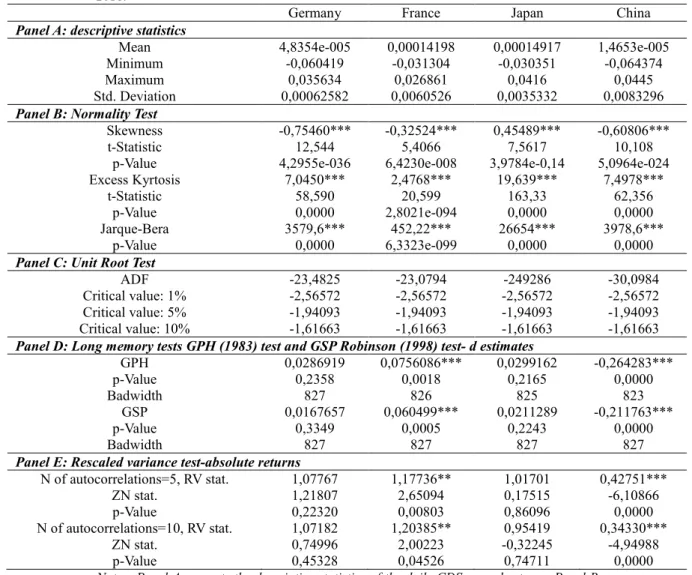
Table 1 below displays the summary statistics for CDS spread returns. While all CDS market returns are skewed to the left, Japan market returns are skewed to the right. Interestingly, China returns exhibit larger fluctuations compared to the rest market returns, according to the higher standard deviation, the highest maximum and the lowest minimum return prices, foreshadowing the results of contagion effects. Additionally, all market returns present excess kurtosis, suggesting leptokurtic behavior (fat tails). Based on the Jarque-Bera statistic, we reject the null hypothesis of normality for all market returns, suggesting the use of student-t distribution as the most appropriate for the empirical analysis (Dimitriou, Kenourgios and Simos 2013; Forbes and Rigobon 2002). All of the market returns were subjected to unit-root testing using Augmented Dickey Fuller test (ADF) (Dickey and Fuller 1979), showing the rejection of the null hypotheses of unit root at 1% level and indicating the daily market returns appropriate for further testing. Furthermore, GSP and GPH tests reject the null hypothesis of no long memory at 1% level for the returns of France and China, whilst the returns of Germany and Japan exhibit long memory effects. (R/S) test results reject the null hypothesis of long term dependence at 1% level for the returns of China and at 5% level for the returns of France.
Tab. 1 Summary statistics of daily CDS spread returns, sample period: 5 Oct 2011 – 5 Feb 2018.
Germany France Japan China
Panel A: descriptive statistics
Mean 4,8354e-005 0,00014198 0,00014917 1,4653e-005
Minimum -0,060419 -0,031304 -0,030351 -0,064374
Maximum 0,035634 0,026861 0,0416 0,0445
Std. Deviation 0,00062582 0,0060526 0,0035332 0,0083296
Panel B: Normality Test
Skewness -0,75460*** -0,32524*** 0,45489*** -0,60806***
t-Statistic 12,544 5,4066 7,5617 10,108
p-Value 4,2955e-036 6,4230e-008 3,9784e-0,14 5,0964e-024
Excess Kyrtosis 7,0450*** 2,4768*** 19,639*** 7,4978***
t-Statistic 58,590 20,599 163,33 62,356
p-Value 0,0000 2,8021e-094 0,0000 0,0000
Jarque-Bera 3579,6*** 452,22*** 26654*** 3978,6***
p-Value 0,0000 6,3323e-099 0,0000 0,0000
Panel C: Unit Root Test
ADF -23,4825 -23,0794 -249286 -30,0984
Critical value: 1% -2,56572 -2,56572 -2,56572 -2,56572
Critical value: 5% -1,94093 -1,94093 -1,94093 -1,94093
Critical value: 10% -1,61663 -1,61663 -1,61663 -1,61663
Panel D: Long memory tests GPH (1983) test and GSP Robinson (1998) test- d estimates
GPH 0,0286919 0,0756086*** 0,0299162 -0,264283*** p-Value 0,2358 0,0018 0,2165 0,0000 Badwidth 827 826 825 823 GSP 0,0167657 0,060499*** 0,0211289 -0,211763*** p-Value 0,3349 0,0005 0,2243 0,0000 Badwidth 827 827 827 827
Panel E: Rescaled variance test-absolute returns
N of autocorrelations=5, RV stat. 1,07767 1,17736** 1,01701 0,42751*** ZN stat. 1,21807 2,65094 0,17515 -6,10866 p-Value 0,22320 0,00803 0,86096 0,0000 N of autocorrelations=10, RV stat. 1,07182 1,20385** 0,95419 0,34330*** ZN stat. 0,74996 2,00223 -0,32245 -4,94988 p-Value 0,45328 0,04526 0,74711 0,0000
Notes: Panel A presents the descriptive statistics of the daily CDS spread returns, Panel B shows the normality test, Panel C demonstrates the unit root tests. We used intercept and a time trend to generate the ADF statistic. Panel D reveals the Geweke and Porter-Hudak’s (1983) (GPH) test and the Gaussian semi parametric (GSP) test of Robinson (1995). We used the above tests in order to examine the existence of long memory for the absolute daily CDS spread returns. In Panel E we observe the (R/S) tests’ results. We used the (R/S) tests in order to examine the long term dependence. *, ** and *** denote statistical significance at the 10%, 5% and 1% levels, respectively.
4. Empirical results
This section is divided into five subsections. First, in section 5.1., the results from the cDCC-AR(1)-FIGARCH(1,d,1) model are described. Second, section 5.2. presents the estimates of simple correlation analysis. Third, in section 5.3., the estimates of conditional variance and covariance statistics are stated. Fourth, section 5.4. provides an explicit economic analysis based on dynamic conditional correlations (DCCs), whilst in section 5.5., we present the diagnostic tests.
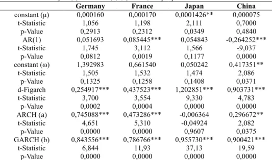
Tab. 2 Estimates of AR(1)-FIGARCH(1,d,1) model, sample period: 5 Oct 2011 – 5 Feb 2018.
Germany France Japan China
constant (μ) 0,000160 0,000170 0,0001426** 0,000075 t-Statistic 1,056 1,198 2,111 0,7000 p-Value 0,2913 0,2312 0,0349 0,4840 AR(1) 0,051693 0,085445*** 0,054843 -0,264252*** t-Statistic 1,745 3,112 1,566 -9,037 p-Value 0,0812 0,0019 0,1177 0,0000 constant (ω) 1,392983 0,661540 0,050242 0,417351** t-Statistic 1,505 1,532 1,474 2,086 p-Value 0,1325 0,1258 0,1408 0,0371 d-Figarch 0,254917*** 0,437523*** 1,202851*** 0,903731*** t-Statistic 3,700 3,554 9,330 4,783 p-Value 0,0002 0,0004 0,0000 0,0000 ARCH (a) 0,745088*** 0,473286*** -0,006364 0,296672** t-Statistic 4,651 5,310 -0,04924 2,082 p-Value 0,0000 0,0000 0,9607 0,0375 GARCH (b) 0,843556*** 0,786766*** 0,955730*** 0,900421*** t-Statistic 6,844 11,93 37,13 19,59 p-Value 0,0000 0,0000 0,0000 0,0000
Notes: Table 3 presents the results of univariate AR(1)-FIGARCH(1,d,1). *, ** and *** denote statistical significance at the 10%, 5% and 1% levels, respectively.
4.1 Results of the cDCC-AR(1)-FIGARCH(1,d,1) model
Table 2 above reports the estimated values for mean equation (Equation 1) and univariate AR(1)-FIGARCH(1,d,1) model11 (Equation 3). Mean
equation exhibits significant μ value only for Japan. The AR(1) is positive for Germany, France, and Japan due to partial adjustment, indicating that
11 The selected lag order (p, d, q) = (1, d, 1) is sufficient for the estimation of conditional
variance as many researchers have mentioned, i.e. Bolleslev, Chou and Kroner (1992), among others.
relevant market information is rapidly reflected in CDS market prices, whilst the negative AR(1) of China suggests the existence of positive feedback, see for instance Antoniou, Koutmos and Pecli (2005). Based on FIGARCH our findings show strong persistent behaviour for all markets (statistically significant d). In addition, all the ARCH (a) and GARCH (b) terms are highly significant except for the ARCH (a) term of Japan.
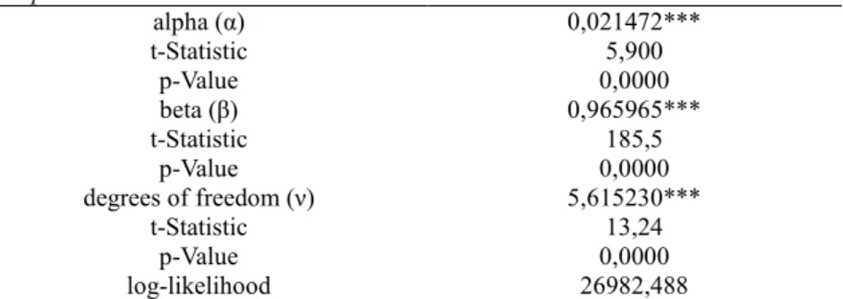
Tab. 3 Estimates of the fourvariate cDCC model, degrees of freedom and log-likelihood, sample period: 5 Oct 2011 – 5 Feb 2018.
alpha (α) 0,021472*** t-Statistic 5,900 p-Value 0,0000 beta (β) 0,965965*** t-Statistic 185,5 p-Value 0,0000 degrees of freedom (ν) 5,615230*** t-Statistic 13,24 p-Value 0,0000 log-likelihood 26982,488
Notes: Panel A shows the results of the conditional correlation driving process Qt, the
degrees of freedom and the log-likelihood. *, ** and *** denote statistical significance at the 10%, 5% and 1% levels, respectively
Table 3 above reports the results of the fourvariate cDCC model estimations (Equation 7 and Equation 9). The cDCC model results show significant α and β parameters, indicating strong ARCH and GARCH effects. This suggests empirical evidence that the CDS markets are integrated (Belke and Gokus 2011). In addition, we provide the estimates of the degrees of freedom (v) and of the log-likelihood.
4.2 Simple Correlation Analysis
In order to measure the financial contagion phenomenon, we implement the Spearman rank correlation approach. If the correlations are statistically significant, we may conclude the existence of transmission mechanisms of shocks between two markets. For a sample size of T observations, the T raw scores -:, •: (i ≠ j = 1,…,N markets and t = 1,…,T observations) are converted
to ranks *, , *,`. Spearman proposes to compute the correlation coefficients
(€•‚ ,•‚ƒ) in the following way: €•‚ ,•‚ƒ =
„…†‡•‚ ,•‚ƒˆ
where Œ)&‡*, , *,`ˆ is the covariance of the rank variables. Additionally,
••‚ and ••‚ƒ are the standard deviations of the rank variables.
Tab. 4 Estimates of Spearman's rank correlation coefficient (€•‚ ,•‚ƒ), sample period: 5 Oct 2011 – 5 Feb 2018.
Market
i Germany (i=1) France (i=2) Japan (i=3) China (i=4)
€•‚ ,•‚ 1 t-Statistic - p-Value - €•‚ ,•‚Y 0,864735*** 1 t-Statistic 47,91 - p-Value 0,0000 - €•‚ ,•‚Ž 0,118823** 0,125056** 1 t-Statistic 2,006 2,274 - p-Value 0,0450 0,0231 - €•‚ ,•‚• -0,002745 -0,007022 0,053556 1 t-Statistic -0,05070 -0,1303 0,9892 - p-Value 0,9596 0,8963 0,3227 -
Notes: Table 5 exhibits the estimates of elements (€•‚ ,•‚ƒ) of rank correlation (Equation 10). *, ** and *** denote statistical significance at the 10%, 5% and 1% levels, respectively.
The empirical results are summarized in Table 4 below. Our evidence show the highest rank correlation for the pairs of markets Germany-France (€•‚ ,•‚Y), Japan-France (€•‚Y,•‚Ž) and Germany-Japan (€•‚ ,•‚Ž),
suggesting a level of integration among Germany, France and Japan. The above results are explained by two main reasons: (1) the membership of Germany and France in the common currency union, and (2) the high exposure of Japan into the European financial market: According to Foreign direct investments (FDIs), Japan has increased the inward investment stock, going from €122 billion in 2008 to more than €200 billion in 2016 (European Commission’s Directorate-General for Trade, 2018). Of particular interest is our finding that the pairs of markets Germany-China(€•‚ ,•‚•),
France-China (€•‚Y,•‚•) and Japan-China (€•‚Ž,•‚•) are not significant, suggesting
4.3 Estimates of conditional variance and covariance statistics
Table 5 below reports the estimated average values (aaaa) of conditional ℎf•
variances and conditional covariances, with i, j = 1,…, N. First we calculate and store the conditional variances and conditional covariances generated by the fourvariate cDCC model. Then, we estimate a regression equation for the conditional variances and conditional covariances on a constant and a trend, generating the conditional variance and covariance statistics. We assume that the average values reflect the own volatility and the cross-volatility spillovers.
Results state strongest own volatility effects for China (ℎaaaaa), Germany ‘‘
(ℎaaaa), France (ℎaaaaa) and Japan (ℎMM aaaaa). Economic conditions of China may ’’
explain the higher own volatility. Global managers invest into Chinese CDS market12, creating turmoil in the CDS market due to the increased concerns
about: (1) an economic slowdown, (2) a property bubble, and (3) the shadow banking system. In addition, Japan13 exhibits the lowest own volatility. This
is interpretable regarding that Japanese CDS market is less exposed compared to other CDS markets globally, considering that companies in Japan prefer more to borrow from banks than to borrow from capital markets. According to the cross-volatility spillovers, we note that ℎaaaa > ℎM aaaa >’
ℎM’
aaaaa > ℎaaaaa > ℎ’‘ aaaa > ℎ‘ aaaaa. The above results suggest that spillover effects for M‘
the pairs of countries Germany-Japan (ℎaaaa), France-Japan (ℎ’ aaaaa) and M’
Germany-France (ℎaaaa) are relatively stronger, indicating that Germany, M
France and Japan are integrated. Two are the major reasons for the higher integration for Germany, Japan and France: (1) the membership of Germany and France in the common currency union and (2) the high exposure of Japan into the European financial market. (European Commission’s Directorate-General for Trade 2018). Furthermore, our evidence suggest the lowest cross-volatility spillovers for the pairs of markets Japan-China (ℎaaaaa), ’‘
Germany -China (ℎaaaa) and France-China (ℎ‘ aaaaa), implying low or no M‘
contagion.
12 Estimates put the total size of the market at over $500bn. China’s government promoted
small and medium-sized enterprises by providing them with credit guarantee, defining China’s CDS market as one of the most popular worldwide.
13 Japan CDS market has traditionally experienced tighter spreads than their USA and
Tab. 5 Average values of conditional variances and covariances (ℎaaaa), sample period: 5 f• Oct 2011 – 5 Feb 2018.
Average St. Deviation Trend (*1000) t-statistic P-value Panel A: Conditional variance statistics
Germany (ℎaaaa) 3,96754e-005 2,19406e-005 -4,75369e-009*** -4,23 0,0000 France (ℎaaaa) MM 3,86536e-005 2,20288e-005 -3,35696e-009*** -2,97 0,0030 Japan (ℎaaaa) ’’ 1,39287e-005 2,33194e-005 7,55481e-010 0,630 0,5291 China (ℎaaaa) ‘‘ 6,76721e-005 8,88338e-005 -6,58625e-008*** -15,4 0,0000 Panel B: Conditional covariance statistics
Germany-France (ℎaaaa) 3,07734e-005 M 1,63941e-005 5,92074e-009*** 7,12 0,0000 Germany-Japan (ℎaaaa) 3,69396e-006 ’ 3,86692e-006 1,70267e-009*** 8,75 0,0000 Germany-China (ℎaaaa) -2,51417e-007 4,09229e-006 ‘ 3,91582e-010 1,86 0,0631 France-Japan (ℎaaaa) 3,50061e-006 M’ 3,76781e-006 1,35679e-009*** 7,10 0,0000 France-China (ℎaaaa) -5,47391e-007 3,50787e-006 M‘ 8,51301e-010*** 4,75 0,0000 Japan-China (ℎaaaa) 1,07559e-006 ’‘ 2,0075e-006 -5,51186e-010*** 5,38 0,0000
Notes: ℎaaaa, with i, j = 1,…,N, denotes the average values of conditional variances and f• conditional covariances. We calculate and store the conditional variances and conditional covariances generated by the cDCC model (Equation 4). Then, we estimate a regression equation for the conditional variances and conditional covariances on a constant and a trend, generating the conditional variance and covariance statistics. *, ** and *** denote statistical significance at the 10%, 5% and 1% levels, respectively.
Figure 2 below plots the behavior of conditional variances for China, France, Germany and Japan. By contacting a visual exploration, we observe that all markets exhibit strong ups and downs over time. France and Germany experience large spikes in the start of the sample period revealing the effects of Eurozone debt crises.
Fig. 2 Conditional variances of the univariate AR(1)-FIGARCH(1,d,1) model
Note: The red lines represent the conditional variance (ℎ:) for all markets, generated by eq 3.
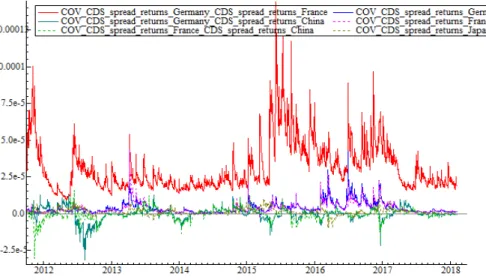
Fig. 3 Conditional covariances of the fourvariate AR(1)-FIGARCH(1,d,1)-cDCC model
Notes: Data from Datastream. The lines illustrate represent the conditional covariances of the fourvariate conditional variance matrix (D:) for all the pairs of markets, generated by eq 4.
Fig. 4 Dynamic conditional correlations of the fourvariate AR(1)-FIGARCH(1,d,1)-cDCC model
Notes: Data from Datastream. The lines illustrate the dynamic conditional correlations (W:), generated by Equation 6 for all the pairs of markets.
In figure 3, we graph the conditional covariances. Results suggest positive values for the conditional covariances between Germany and France, whilst the rest pairs of markets exhibit positive and negative values. Specifically, for the market pairs Germany-Japan, France-Japan and Japan-China conditional correlations stay positive for a longer period, while for the market pairs, Germany-China and France-China conditional correlations stay negative for a longer period.
4.4 Economic analysis of dynamic conditional correlation coefficients
We proceed with the fourvariate AR(1)-FIGARCH(1,d,1)-cDCC’s estimation, using sovereign CDS spread returns of Germany, France, China and Japan against USA, illustrated graphically in Figure 5. The dynamic conditional correlation coefficient (DCC coefficient) estimates aim to give us a much clearer view of contagion effects.
As depicted in figure 4 above, the DCC coefficient between Germany and France are positive and persistently high in two periods (30/09/2013 to 28/02/2017 and 28/07/2017 to 5/02/2018), foreshadowing interdependence
phenomenon, see for instance, Forbes and Rigobon (2002). The membership of Germany and France in Eurozone rationalizes the strong economic interdependence between the two countries. Moreover, DCC coefficient is positive and highly volatile in the two periods (6/08/2011 to 29/09/2013 and 01/03/2017 to 27/07/2017), implying contagion effects and generating two important ramifications from the investor’s perspective. First, a highly volatile DCC coefficient implies that the stability of the correlation is less reliable in guiding portfolio decision. Second, a DCC coefficient with positive values suggests that the benefit from market-portfolio diversification becomes less, since holding a portfolio with diverse sovereign CDS premiums for Germany and France is subject to systematic risk. Furthermore, DCC coefficient exhibits two main jumps over time (28/11/2012, 23/04/2017) considering the European Commission’s approval of Spanish government's plan to shrink and restructure three major Spanish banks and sell a fourth (28/11/2012) and the French Presidential elections14
(23/04/2017).
Next, the DCC coefficients for the pairs of countries Germany-Japan and France-Japan exhibit strong co-movements, since Germany and France are Eurozone members and they are economically interdependent. Although DCC coefficients are positive and extremely volatile over time, they present some signs of negative values, providing evidence of contagion effects that imply increasing riskiness from an investor’s point of view. In addition, DCC coefficients demonstrate three common extreme jumps (07/01/2015, 20/09/2015, 23/06/2016) that can be attributed to: (a) Charlie Hebdo attack in Paris (07/01/2015), (b) Greek domestic conditions e.g. legislative elections (20/09/2015), and (c) the United Kingdom European Union membership referendum (23/06/2016). The above economic events may have caused short-term global markets drop.
Moreover, the DCC coefficients for the pairs of countries Germany-China and France-China demonstrate strong co-movements justified by the membership of Germany and France in Eurozone. However, DCC coefficients stay negative for a long period and they are extremely volatile. Additionally, DCC coefficients present some common jumps over time with some of the most important generated by short-term global market drops of the following economic facts: (a) the 19bn euros worth bailout of Spain's fourth largest bank, Bankia (25/05/2012), (b) the day The President of the Catalonia, Artur Mas i Gavarró dropped plans for a referendum on independence on 9/11/2014 from Spain (14/10/2014), and (c) the European
14 In 23rd April 2017 took place the first round of the French Presidential Elections of
2017. Emmanuel Macron, who received 24 % of the first round vote, and Marine Le Pen, who received 21.3 %, received the highest vote shares.
Central Bank announcement of an aggressive money-creation program, printing more than one trillion new euros (22/01/2015).
Figure 4 show that the DCC coefficient between Japan and China are mainly positive, however are extremely volatile over time, indicating a low stability of the correlation. Interestingly, we observe some extreme jumps over time (30/03/2015, 02/04/2016) including jumps generated by major economic events, i.e. (a) on 30/03/2015, the BOJ decided to keep in place its massive easing program of purchasing 80 trillion yen ($670 billion) worth of assets annually, and (b) foreign investors bought a net of ¥ 415.2 billion worth of Japanese stocks in the week that ended 02/04/2016 bringing an end to 12 weeks of net selling, among others.
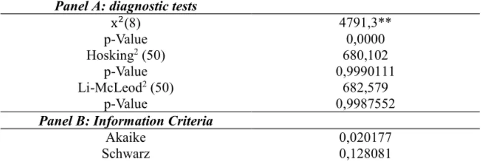
Tab. 6 Estimates of diagnostic tests and information criteria, sample period: 5 Oct 2011 – 5 Feb 2018.
Panel A: diagnostic tests
xM(8) 4791,3** p-Value 0,0000 Hosking2 (50) 680,102 p-Value 0,9990111 Li-McLeod2 (50) 682,579 p-Value 0,9987552
Panel B: Information Criteria
Akaike 0,020177
Schwarz 0,128081
Notes: Panel A demonstrates the diagnostic tests of Hosking (1980) and McLeod and Li (1983). In Panel B we see the information criteria of AR(1)-FIGARCH(1,d,1)-cDCC model. The symmetric positive definite matrix ^: is generated using one lag of Q and of .∗. P-values have been corrected by 2 degrees of freedom for Hosking2 (50) and Li-McLeod2 (50) statistics.
*, ** and *** denote statistical significance at the 10%, 5% and 1% levels, respectively.
4.5 Diagnostic tests, hypothesis testing & information criteria
Ηypothesis testing results and information criteria are exhibited in table 6 above, •M(8) statistic results suggest that the null hypothesis of no spillovers is rejected at 1% significance level. In addition, Ljuing-Box test results (Hosking 1980; Li-McLeod 1983) provide evidence of no serial autocorrelation, suggesting the absence of misspecification errors of the estimated MGARCH model. Furthermore, AIC and SIC information criteria are provided for our model.
5. Conclusions
In this article, we study the volatility transmission among 20-year maturity sovereign CDS markets using data for USA, Germany, France, Japan and China for the period 2011 – 2018. We apply a fourvariate cDCC-AR(1)-FIGARCH(1,d,1) framework suggested by Aielli (2009). To the best of our knowledge no empirical study has attempted to analyze the volatility effects among the under investigation sovereign CDS markets in order to quantify and measure potential contagion effects.
We find interesting results. According to the Spearman’s rank correlation coefficient financial contagion exists in the country pairs: Germany-France, Germany-Japan and France-Japan, whilst the pairwise correlations between China with the rest countries indicate low or no contagion. Next, we estimate the conditional variance and covariance statistics. Results suggest contagion effects in the pairs: Germany-France, Germany-Japan and France-Japan and China proved to be extremely volatile. Then, we have extended our analysis by considering the DCC coefficients between CDS markets. DCCs analysis state evidence of contagion for the pairs of markets Germany-France, Germany-Japan and France-Japan.
Our empirical findings are important for investors and policy makers. Investors can use the information about the contagion effects among the above markets, quantify the risk, and gain the flexibility to top-up their investments in CDS market at any time. They should be cautious about simultaneously investing into markets that exhibit contagion effects. Furthermore, the policy makers should examine possible strategies that take into account the spillover effects of the above markets during future crises that can arise in the global CDS markets.
References
Aielli, G. P. (2009). Dynamic conditional correlations: on properties and estimation. Technical report, Department of Statistics, University of Florence.
Anderson, M. (2010). Contagion and Excess Correlation in Credit Default Swaps. Working Paper, Department of Finance, Fisher College of Business, Ohio State University.
Antoniou, A, Koutsmos, G., & Percli, A. (2005). Index futures and positive feedback trading: evidence from major stock exchanges. Journal of Empirical Finance, 12(2), 219-238. Baillie, R. T., Bollerslev, T. & Mikkelsen, H. O. (1996). Fractionally integrated generalized autoregressive conditional heteroskedasticity. Journal of Econometrics, 74(1), 3-30.
Belke A., & Gokus, C. (2011). Volatility Patterns of CDS, Bond and Stock Markets before and during the Financial Crisis Evidence from Major Financial Institutions. Working Papers, Deutsches Institut fur Wirtschaftsforschung.
Blanco, R., Brennan, S., & Marsh, I. W. (2005). An Empirical Analysis of the Dynamic Relation between Investment-Grade Bonds and Credit Default Swaps. The Journal of Finance, 60(5), 2255-2281.
Bollerslev, T., Chou, R., & Kroner, K. F. (1992). ARCH modeling in finance: A review of the theory and empirical evidence. Journal of Econometrics, 52(1-2), 5-59.
Calice, G., Chen, J., & Williams, J. (2011). Liquidity Spillovers in Sovereign Bond and CDS Markets. Paolo Baffi Centre Research Paper.
Caporale, G. M., Pittis, N., & Spagnolo, N. (2006) Volatility Transmission and Financial Crises. Journal of Economics and Finance, 30(3), 376-390.
Chen, K, Fleming, M., Jackson, J., Li, A., & Sarkar, A. (2011). An Analysis of CDS Transactions: Implications for Public Reporting. Federal Reserve Bank of New York, Staff Reports, 517.
Chen, L., Lesmond, D. A., & Wei, J. (2007). Corporate Yield Spreads and Bond Liquidity. Journal of Finance, 62(1), 119-149.
Dickey, D. A., & Fuller, W. A. (1979)) Distribution of the Estimators for Autoregressive Time Series with a Unit Root. Journal of the American Statistical Association, 74, 427-431.
Didier, T., Mauro, P., & Schmuckler, S. (2008). Vanishing financial contagion?. Journal of policy modeling, 30, 775-791.
Dimitriou, D, Kenourgios, D., & Simos, T. (2013). Global financial crisis and emerging stock market contagion: A multivariate FIAPARCH-DCC approach. International Review of Financial Analysis, 30, 46-56.
Engle, R. F. (2002). Dynamic conditional correlation: a simple class of multivariate generalized autoregressive conditional heteroskedasticity models. Journal of Business and Economic Statistics, 20, 339-350.
European Commission’s Directorate-General for Trade (2008): The economic impact of the EU-Japan economic partnership agreement (EPA). European Commision.
Fonseca, J. D., &Gottschalk, K. (2012). The Co-movement of Credit Default Swap Spreads, Stock Market Returns and Volatilities: Evidence from Asia-Pacific Markets. Tech. rep., Working Paper, May 31.
Forbes, K. J., & Rigobon, R. (2002). No Contagion, Only Interdependence: Measuring Stock Market Comovements. The Journal of Finance, 57(5), 2223-2261.
Hull, J.C.(2008). Options, Futures and Other Derivatives. 6th edition, Prentice Hall. Koseoglu, S. D. (2013). The Transmission of Volatility between the CDS Spreads and Equity Returns Before, During and After the Global Financial Crisis: Evidence from Turkey. Proceedings of 8th Asian Business Research Conference 1 - 2 April 2013, Bangkok, Thailand. Lake, A., & Apergis, N. (2009). Credit default swaps and stock prices: Further evidence within and across markets from mean and volatility transmission with a MVGARCH-M model and newer data. University of Pireaeus.
Meng, L., Gwilym, O., & Varas, J. (2009). Volatility Transmission among the CDS, Equity, and Bond Markets. Journal of Fixed Income, 18(3), 33-46.
Sarig, O., & Warga, A. (1989). Some empirical estimates of the risk structure of interest rates. Journal of Finance, 44(4), 1351-1360.
Schreiber, I., Müller, G., Klüppelberg, C., & Wagner, N. (2009). Equities, Credits and Volatilities: A Multivariate Analysis of the European Market During the Sub-prime Crisis. in: Working Paper, TUM, University of Passau, Germany, in: http://ssrn.com/abstract=1493925, accessed on: January 02, 2013.
Stevens, G. (2008). Economic prospects in 2008: An antipodean view. Address by the Governor of the Reserve Bank of Australia to Australian Business, January 18, London, UK. Tokat, H. A. (2013). Understanding volatility transmission mechanism among the cds markets: Europe & North America versus Brazil & Turkey. Economia Aplicada, 17(1).
Watzka, S., &Missio, S. (2011). Financial Contagion and the European Debt Crisis. CESIFO working paper. No. 3554.
Wei, C. C. (2008). Multivariate GARCH Modeling Analysis of Unexpected USD, Yen and Euro-Dollar to Reminibi Volatility Spillover to Stock Markets. Economics Bulletin, 3(64), 1-15.
Worthington, A.C., & Higgs, H. (2003). A Multivariate GARCH Analysis of the Domestic Transmission of Energy Commodity Prices and Volatility: A Comparison of the Peak and Off-Peak Periods in the Australian Electricity Spot Market. Queensland University of Technology, School of Economics and Finance, Discussion Paper No: 140.
Zhu, L., & Yang, J. (2004). The Role of Psychic Distance in Contagion: A Gravity Model for Contagious Financial Crises. Working Paper, The George Washington University.