UNIVERSITY
OF TRENTO
DIPARTIMENTO DI INGEGNERIA E SCIENZA DELL’INFORMAZIONE
38050 Povo – Trento (Italy), Via Sommarive 14
http://www.disi.unitn.it
ACHIEVING PERFORMANCE AND ROBUSTNESS IN P2P
STREAMING SYSTEMS
Luca Abeni, Csaba Kiraly and Renato Lo Cigno
July 2009
TR-DISI-09-041: Achieving Performance and
Robustness in P2P Streaming Systems
Luca Abeni, Csaba Kiraly, Renato Lo Cigno
DISI – University of Trento, Italy
[email protected],
{csaba.kiraly,renato.locigno}@disi.unitn.it
July 29, 2009
Abstract
This paper present a thorough and homogeneous comparison of chunk and peer selection strategies suitable for mesh-based, live, P2P streaming applications. Strategies are studied in a context of push protocols, and it is shown that none of the schedulers analyzed, which are, to the best of our knowledge, the majority of those proposed in the literature, offer acceptable performances on a range of scenarios commonly encountered in networks. Results also show that the key weakness is in the peer selection strategy. Based on these observations, we propose a new peer se-lection strategy which blends together an optimal peer sese-lection for homogeneous networks with a bandwidth aware approach. Extended experiments show that un-der all the scenarios consiun-dered this peer scheduler performs consistently better than all the others, specially when coupled with a deadline-based, robust chunk selection strategy.
1
Introduction
Live streaming is becoming one of the most active research areas in P2P systems, in part because of its commercial importance, with P2P-TV systems spreading on the Internet, and in part because of its challenging research topics that stimulate the com-munity. One of the challenges in research is the information scheduling strategy in un-structured, mesh-based systems, which includes decisions on which information piece is distributed to (or retrieved from) which peer in the system.
There are several reasons why this topic is extremely important and is receiving a lot of attention: i) it is one of the main driver of the system performance; ii) efficient and performing distributed solutions are difficult to find due to the dynamic nature of the overlay topology and due to the tight deadlines typical of real-time systems; and iii) when the stream is video, the networking resources required are large and interaction of the overlay application with the underlying network play a crucial role in both performance and efficiency.
We are not concerned here on whether unstructured systems are better than struc-tured ones (see [3] or [10] for examples), or with the definition of any specific protocol
for the exchange of information. We assume the system is unstructured and there is a topology management function that builds a neighbourhoodNi, which is the
knowl-edge base (peers address, its characteristics, the information it owns, etc.) used by peer Pi to take its scheduling decisions. Moreover we restrict the scope of the paper to
chunk1based, push systems, once more without assuming that they are better or worse than pull ones or of systems where information is not chunk-ized, but grouped with a different approach (frames, layers, . . . ). We focus on the algorithmic choices and deci-sions regarding the selection of peers and chunks and the effects of coupling different algorithms for peer and chunk selection and the order they are applied (i.e., chunk first or peer first).
What complicates the scenario is that networks are not ideal, neither homogeneous, so that the choice of the peer will affect the performance in transferring the chunk to it, but also how this specific chunk will be diffused in the future: peers more endowed with resources will diffuse the chunk more efficiently than peers with scarce resources. Until very recently, literature on chunk and peer scheduling was based on heuristics of-ten embedded and indistinguishable from the protocol to exchange the information (see Section 7 for a discussion of the literature), and normally overlooked both fundamental bounds to be compared with, and the interaction between the application and the net-work. Recently two works started looking at the problem with a different perspective. In [4] the resources (in terms of bandwidth) of the selected peer were included in the selection procedure, showing that in some heterogeneous scenarios this is fundamental to achieve good performance. Even more recently, [1] proved the existence of a class of distributed algorithms that in ideal networking scenarios achieve optimal distribution delay for a streaming system, thus setting a clear bound against which comparisons can be made in realistic scenarios.
As in [4], we consider the upload bandwidth of peers as their dominant character-istic, i.e., we disregard the impact of the difference in delay between peers and we as-sume that download bandwidth of peers is always much larger than upload bandwidth, so that performance is dominated by this latter, apart, obviously, from the scheduling decisions. We address both full mesh topologies, to understand basic properties of the algorithms, and general, random topologies characterised by a reduced neighbourhood size as they can emerge from a gossipping protocol like NewsCast [9] to understand the impact of realistic neighborhood sizes. Finally, we consider both the limiting case of average upload bandwidth equal to the stream bandwidth, where algorithms’ properties are stressed and highlight their properties, and the impact of increased resources in the network.
The contributions of this paper are two:
1. On the one hand, we explore and assess the performance of a number of pos-sible chunk and peer scheduling algorithms known in the literature, taking into account their combination as peer or chunk first as well as different bandwidth models and inhomogeneity in their distribution, up to the extreme case of large bandwidth peers coupled with “free-riders” due to the lack of resources; 2. On the other hand, we propose a peer selection algorithm that blends
teristics of the optimal scheduler proposed in [1] with the bandwidth awareness proposed in [4] in a joint scheduler that proves to be robust and performs better than any other scheduler in all analysed scenarios.
The remaining of the paper is organised as follows. Section 2 introduces the no-tation we use and defines clearly the main algorithms for peer and chunk scheduling found in the literature. Section 3 defines the networking model and the different band-width distribution functions that we use in performance evaluation. Section 4 presents a set of results that show how none of the schedulers defined so far is able to per-form well in a wide range of conditions, triggering the search for a novel scheduler, described in Section 5, the Bandwidth-Aware Earliest-Latest peer (BAELp) scheduler. This is the scheduler, we define and propose in this paper as the most robust blend of network-awareness and optimality2. Section 6 presents results that demonstrate how this BAELp performs consistenly better than any other scheduling combination when combined with a deadline-based chunk scheduler. Section 7 discusses the remaining literature relevant to this paper and Section 8 closes the paper with discussions on its contributions.
2
Schedulers Definition and Composition
An unstructured P2P streaming system is modelled as a setS = {P1, . . . PN} of N
peersPi, whose aim is receiving a stream from a source, which is a peer itself, but
‘special’ in that it does not need to receive the stream, so is is not part ofS. The media stream is divided inMcchunks; each peerPireceives chunksCjfrom other peers, and
sends them out at a rates(Pi). The set of chunks already received by Pi at timet is
indicated asC(Pi, t). The most important symbols used in this paper are recalled in
Table 1.
The source generates chunks in order, at a fixed rateλ and sends them with rate s(source) = λ, i.e., the source emits only one copy of every chunk. All the bitrates are normalised w.r.t.λ, so that the generation time of Cjisrj= j.
IfDj(t − rj) is the set of nodes owning chunk Cjat timet, the worst case diffusion
delayfj of chunkCj is formally defined as the time needed byCj to be distributed
to every peer: fj = min{δ : Dj(δ) = S}. According to this definition, a generic
peerPiwill receive chunkCj at timet with rj + 1 ≤ t ≤ rj+ fj. Considering an
unstructured overlayt will be randomly distributed inside such interval. Hence, in an unstructured systemPiis guaranteed to receiveCjat most at timerj+fj. To correctly
reproduce the whole media stream, a peer must buffer chunks for a time of at least F = max1≤j≤Mc(fj) before starting to play. For this reason, the worst case diffusion delayF is a fundamental performance metric for P2P streaming systems, and this paper will focus on it. We will also consider the 90 percentile over chunks of the diffusion time, which is important, for instance, when FEC or any form of redundant coding is used3. The average delay is instead not very meaningful in streaming systems, since 2The Earliest-Latest (ELp) scheduler was proven to be the optimal peer selection strategy under
homo-geneous and ideal networking scenario in [1].
3Other percentiles, like 95, 99, or even 80 can be considered, depending on the specific redundancy of
Symbol Definition S Set of all the peers
N Number of peers in the system Mc Number of chunks in the stream
Pi Theithpeer
Ch Thehthchunk
rh Time when the source generatesCh
Ni Neighbourhood of peerPi
NN Neighbourhood size
fh Diffusion delay ofCh
(time needed byChto reach
all the peers)
C(Pi, t) Set of chunks owned byPiat timet
C′(P
i, t) Set of chunks owned byPiat timet which
are needed by some ofPi’s neighbours
s(Pi) Upload bandwidth ofPi
Table 1: Symbols used in the paper for the main system parameters.
the playout buffer must be dimensioned based on the most delayed piece of information otherwise it can empty during playout and the video must annoyingly stop waiting for new information to fill the buffer.
Whenever a peerPi decides to contribute to the streaming and pushes a chunk, it
is responsible for selecting the chunk to be sent and the destination peer. These two decisions form the scheduling logic, and they are taken by two schedulers: the chunk
scheduler, and peer scheduler. The peer scheduling algorithm can select a target peer
Pk ∈ Ni, whereNiis the set of its neighbours (the neighbourhood). The case in which
∀i, Ni = S − Pi corresponds to a fully connected graph, and, albeit not realistic, it
is useful to explore elementary properties of different scheduling logicsx. Given an Xchunk scheduler and a Y peer scheduler, applying first X and then Y one obtains a
chunk-first X/Yscheduler; the other way around one obtains a peer-first Y/X scheduler.
The chunk and peer scheduling algorithms can be blind (a peer does not use any information about the chunks received by its neighbours), or can be based on some knowledge about the status of the neighbours themselves. In the following, we briefly define the scheduling algorithms evaluated in this paper, referring to the relevant liter-ature when appropriate.
2.1
Chunk Schedulers
Random Blind (RBc) Pirandomly selects a chunkCj ∈ C(Pi, t) regardless of its
possible usefulness for the peers inNi.
Random Useful (RUc) Pi randomly selects a chunk Cj ∈ C′(Pi, t) based on the
Latest Blind (LBc) Piselects the most recent chunkCj ∈ C(Pi, t) (that is, the one
having the largest generation time), regardless of its possible usefulness for the peers inNi.
Latest Useful (LUc) Piselects the most recent chunkCj∈ C(Pi, t) (that is, the one
having the largest generation time) that is needed by some of the peers inNi.
Deadline-based scheduler (DLc): Pi selects the chunk Cj ∈ C(Pi, t) having the
earliest scheduling deadline. Scheduling deadlines are assigned to the various chunks instances present in the system, and each scheduling deadline is postponed by a fixed amount when sending a chunk. The amount of deadline postponing is a parameter of the algorithm, and is generally assumed to be2 times the chunk size. This algorithm [1] has been proved to be optimal in full meshes (like LUc), and to generally provide good performance when the neighborhood size is reduced (hence, is is claimed to be robust, unlike LUc).
Since the non-blind algorithms (DLc, LUc and RUc) are known from the literature to perform better than blind ones, this paper will only consider non-blind algorithms.
2.2
Peer Schedulers
Random Useful Peer (RUp) Pirandomly selects a peer inNithat needs the selected
chunk (or a generic chunkCj ∈ C(Pi, t) if the peer is selected first).
Most Deprived Peer (MDp) Piselects the peerPjinNi which owns the smallest
number of the chunks currently owned byPi[6].
Earliest Latest scheduler (ELp) Piselects the target peer owning the earliest latest
chunk [1]. See Section 5 for a description of the algorithm.
Both ELp [1] and MDp [6] have been proved to have some optimality properties (see the original papers for more details), hence in this paper they are considered in all the scheduling performance evaluation because of their formal properties.
As already noticed in [5, 4], to be effective in a heterogeneous system a peer sched-uler must consider the output bandwidth of the various peers. This is the idea of
Band-width Awarepeer scheduling, which tends to select as targets the peers with higher
output bitrate (as they are supposed to contribute more to the chunk diffusion).
Bandwidth Aware scheduler (BAp w) Pirandomly selects a target peerPk ∈ Ni
3
Network and Bandwidth Models
Assessing performances in an heterogeneous network requires a network . . . or a model of it. For our results we use a simulation tool developed within an EU project4. The
simulator allows describing bandwidths and delays between peers and building many overlay topologies.
We restrict the analysis to the case when bandwidths are a property of the single peer and the overlay topology is n-regular5. The bandwidth being a property of the
peer is typical of cases when the bottleneck is on the access link, normally the upload, regardless of it being due to physical constraints or user choices. We use either full meshes or n-regular topologies; other overlay topologies can be studied, but prelimi-nary results indicate that streaming performance is not much influenced by the specific characteristics of the topology as far as it remains reasonably random and with good connectivity, i.e.,NN > log2(N ), and with good random properties. Delays between
peers are random, and for the time being we assume perfect knowledge of the neigh-bourhood status, which correspond to situations when the delays are small compared to chunk transmission times. The download bandwidth of a peerPi is assumed to be
much larger than its upload bandwidths(Pi).
Since the upload bandwidths of peersPi∈ S are not homogeneous, it is important
to model their distribution. We consider two possible bandwidth distributions:
class-based distributions(such as may arise from ADSL links), and continuous distributions
(that may arise from user-imposed constraints). In a class-based distribution, the peers are grouped in a finite number of classes, and every class of peers is characterised by a different upload bandwidth. In a continuous distribution, the upload bandwidth of every single peer is randomly assigned according to a specified Probability Density Function (PDF).
Various models of class-based and continuous bandwidth distributions have been tested and simulated. We consider results generated in three different scenarios re-ferred as “3-class”, “uniform”, and “free-riders”. The 3-class scenario is based on a class-based distribution with three classes: low-bandwidth peers (having an upload bandwidth equal to0.5B), mid-bandwidth peers (having an upload bandwidth equal to B), and high-bandwidth peers having an upload bandwidth equal to 2B. The fraction of high-bandwidth peers in the system ish/3 (where h is an heterogeneity factor), the fraction of low-bandwidth peers is2h/3, and the fraction of mid-bandwidth peers is 1 − h; as a result, the average bandwidth is
2B · h/3 + B · (1 − h) + 0.5B · 2h/3 = B .
This scenario has been selected because it captures the most important properties of a class-based distribution, and a similar setup has already been used in literature [2].
The uniform scenario is an example of continuous distribution, in whichs(Pi) is
uniformly distributed between a minimum valueBmin = (1 − H)B and a maximum 4We refrain from indicating its download page due to double blind review, however the tool is freely
available to the community and will be disclosed in the final version of the paper.
5In n-regular topologies all nodes have the same connectivity degree, which means that the
valueBmax= (1 + H)B, where B is the average upload bandwidth and H is again an
heterogeneity factor, indicated with capitalH instead of small h because the stochastic
properties of the 3-class and the uniform scenario are not equal for an equal value of the heterogeneity factor. This scenario is particularly interesting because it allows to check if some of the properties and results noticed in the 3-class scenario are due to artifacts caused by a class-based distribution, or are generic properties. Different kinds of continuous PDFs have been tested, and the uniform one is used in this paper because it seems to capture most of the generic properties observed using other kinds of PDFs. Finally, the free-riders scenario is based on a two-class distribution in which one class of peers is composed by “free riders”, having upload bandwidth equal to0. This scenario is important as it allows to understand what happens when some of the peers for some reasons do not contribute to the chunks diffusion.
4
The Quest for a Robust Scheduler
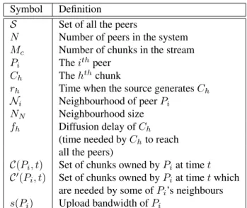
1e-06 1e-05 0.0001 0.001 0.01 0.1 1 0 100 200 300 400 500 600 700 800 900 1000
Chunk loss probability
Playout delay
peers=600; degree=14; chunks=1000; 3-class scenario, h=0.15
LUc-RUp LUc-ELp LUc-MDp LUc-BAp RUc-RUp RUc-ELp RUc-MDp RUc-BAp DLc-RUp DLc-ELp DLc-MDp DLc-BAp
Figure 1: Probability to drop a chunk as a function of the playout delay (D); chunk first schedulers.
Each of the schedulers presented in Section 2 has been found, in some context or another, to perform well. However, a scheduling logic composing a peer and a chunk scheduler must be, first of all, robust to different network conditions, rather than performing well in one context and badly in another. We have evaluated all the schedulers under many conditions through extensive simulations: The amount of data
1e-06 1e-05 0.0001 0.001 0.01 0.1 1 0 100 200 300 400 500 600 700 800 900 1000
Chunk loss probability
Playout delay
peers=600; degree=14; chunks=1000; 3-class scenario, h=0.15
RUp/LUc ELp/LUc MDp/LUc BAp/LUc RUp/RUc ELp/RUc MDp/RUc BAp/RUc RUp/DLc ELp/DLc MDp/DLc BAp/DLc
Figure 2: Probability to drop a chunk as a function of the playout delay (D); peer first schedulers.
produced during such simulations is so large (hundreds of plots!) that it is important to identify the most relevant results, and to focus on them. In particular, it is important to understand:
• Which metric to use for comparing the algorithms;
• What algorithms are the best candidates for further refinement and development; • Whether there is a clear advantage in using a CTL based on chunk- or peer-first
strategy.
The first batch of simulations, presented in this section, is dedicated to understand these three major issues.
In some previous works, different scheduling algorithms were compared using the
averagechunk diffusion time as a metric. This make sense, because such a metric
allows to evaluate the long-term stability of a streaming system, and gives an ideas of the average performance. However, using the average diffusion time to predict the QoS experienced by a user is not easy, because it does not provide enough information about the chunks dropped in the system, or delayed beyond thir target playout time. As noticed in Section 2, the probability to drop a chunkCjdepends on the chunk diffusion
timefj: iffj is larger than the playout delay, thenCj is dropped. If some chunk loss
can be tolerated, then the metric to be measured is some percentile (depending on the percentage of lost chunks that can be tolerated). If error correction is used (such as
FEC), then more lost chunks can be tolerated: for example, with a FEC providing10% of redundancy, the most important metric is the90-th percentile, possibly coupled with the correlation function of losses. Moreover, the chunk delay distribution is hard to predict and definitively non-linear, so that different algorithms can behave differently when the average, maximum, the median, or any other percentile is considered.
Figures 1 and 2 plot the probabilityP {δ > D} for a chunk to have a diffusion time δ larger than the playout delay D. P {δ > D} is the probability to drop a chunk (note that this probability is equal to1−CDF, where CDF is the Cumulative Distribution Function of the chunk diffusion times). The networking scenario is the following: N = 600 nodes, Mc = 1000 chunks, connectivity degree NN = 14, 3-class scenario
withh = 0.15, and the simulations have been repeated for a number of chunk-first Figure 1 and peer-first Figures 2 algorithms.
The first observation is that the distributions of different algorithms cross one an-other, sometimes more than one time, so that chosing a specific point of the distribu-tion, such as the average or maximum does influence the result of the comparison, as predictable from the theoretical characteristics of schedulers (e.g., LUc is optimal but fragile to the connectivity degree reduction). Given the nature of the application, we will use the maximum and 90-th percentile of delay as dominant parameters, but with the warning that, to gain insight in schedulers’ performance it is often necessary to analyse the entire distribution correlated to the relevant parameter under study.
Figure 1 plots all chunk-first schedulers, while Figure 2 plots all peer-first sched-ulers. Comparing all chunk-first X/Y scheduling strategies with the dual peer-first Y/X scheduling strategy it is clear that chunk-first CTL performs consistently better, and this justify the decision to restrict the presentation of results in the remaining of the paper to chunk-first strategies.
Inspecting Figure 1, it is possible to see that although the LUc chunk scheduler provides small average diffusion times (some more focused experiments show that it provides the smallest average diffusion times), its CDF has a long tail and the worst case diffusion time is very large. It is also possible to notice that DLc (and in particular DLc/ELp) provides the best performance.
To be sure that the results previously described are not the effect of some artifact introduced by a specific scenario, and do not depend on a particular bandwidth distri-bution, a set of experiments has been run with different scenarios, and the results were consistent with the previous ones. For example, Figure 3 reports the 90-th percentile of the chunk diffusion delay using the same settings as above, but in a full mesh instead that with limited neighbourhood, and in a uniform scenario (as described in Section 3) with average bandwidthB = 1. The plot are function of the bandwidth variability H, with H = 0 corresponding to a homogeneous scenario (Bmin = Bmax = 1
andH = 1 corresponding to the peers upload bandwidths uniformly distributed in [Bmin= 0, Bmax= 2].
Analysing the figure it is clear that LUc and DLc chunk schedulers ensure the best performance (but LUc is fragile reducing the neighbourhood size), while in peer scheduling there is no clear winner: bandwidth awareness guarantees good perfor-mances in highly non homogeneous scenarios, while ELp performs the best (as it must be) in case of homogeneous networks.
10 20 30 40 50 60 70 80 0 0.2 0.4 0.6 0.8 1 90% diffusion time H (heterogeneity) average BW=1.0
peers=600; degree=599; chunks=1200
LUc/RUp LUc/ELp LUc/MDp LUc/BAp_w RUc/RUp RUc/ELp RUc/MDp RUc/BAp_w DLc/RUp DLc/ELp DLc/MDp DLc/BAp_w
Figure 3: 90-th percentile of delay for selected chunk-first schedulers as a function of the bandwidth variability in the 3-class scenario.
the most promising to obtain robust yet performant scheduling procedures. For this reason, and because of its formal optimality in full meshes, this paper will use DLc as a chunk scheduler and will focus on comparing different peer schedulers. Moreover, in case of homogeneous or mildly inhomogeneous networks scheduling peers based on ELp proves to be the best solution, while in case of high inhomogeneity, bandwidth aware peer selection gives an advantage.
These observations push us to seek and define a peer-scheduler that blends together the proven optimality of ELp in case of homogeneous networks with the smartness of chosing bandwidth endowed peers in case of heterogeneous networks.
5
A Bandwidth-Aware ELp Algorithm
As previously noticed, to be effective in an heterogeneous scenarios a peer scheduling algorithm must consider the output rate of the target peer. Some scheduling algo-rithms [4] only consider the output rate of the target peer, while other algoalgo-rithms [5] propose some sort of hierarchical scheduling, in which a set of peers is first selected based on the output rates, and a peer is then selected in this set based on other informa-tion.
As highlighted in Section 4, a peer scheduler, in order to be robust to different bandwidth distribution scenarios, should be both bandwidth aware and select peers
function L(Pk, t) max= 0 for allChinC(Pk, t) do ifrh> max then max =rh end if end for return max end function functionELP(Pi, t) int min; peer target; for allPkinNido if L(Pk, t)< min then min = L(Pk, t); target =Pk; end if end for return target end function
Figure 4: The ELp algorithm.
that are in the best conditions to redistribute the chunk as ELp does [1]. ELp has been proved to be optimal for the uniform bandwidths case and is defined in Figure 4. In practice, ELp selects the target peer having the latest chunkCh with the earliest
generation timerh.
A first way to integrate ELp with some kind of bandwidth awareness is to use hi-erarchical scheduling. Two possible hihi-erarchical combinations can be implemented: ELhBAp and BAhELp. ELhBAp uses ELp to select a set of peers having the earliest latest chunk, and then uses a bandwidth aware strategy to select the peer having the highest output bandwidth among them. On the other hand, BAhELp first uses a band-width aware scheduler to select the set of peers having the highest output bandband-widths and then applies ELp scheduling to this set.
Although hierarchical scheduling can be very effective in some situations, some-times better integration of the two scheduling algorithms can improve the system’s performance (as it will be shown in Section 6). To understand how to integrate ELp and bandwidth aware scheduling, it is important to better understand the details of earliest-latest scheduling.
LetL(Pi, t) be the latest chunk owned by, or in arrival to, Piat timet. ELp
min-imisesL(Pj, t), and this is equivalent to maximising t − L(Pj, t). The meaning of this
rule is that ELp tries to select the target peerPihaving the latest chunk that has been
sent more times (hence, it can be argued that such a chunk will be useful for less time, and the peer can soon pass to redistribute another one). However, the peer status at
15 20 25 30 35 40 45 50 55 0.01 0.1 1 10 100
max diffusion time
weight w associated to banwidth information Combining BA and ELp,
3-class scenario with average BW=1.0, h=0.5 peers=1000; degree=20; chunks=10000; playout delay=50
LUc/BAxELp DLc/BAxELp DLc3/BAxELp DLc5/BAxELp DLc10/BAxELp RUc/BAxELp
Figure 5: BAELp sensitivity tow: Worst Case Diffusion Time, neighbourhood size 20, 3-class scenario withh = 0.5.
will be received. The original ELp algorithm has been developed assuming that all the peers have the same output bandwidths(Pj) = 1, so every chunk was diffused in 1
time unit and the quantity to be maximised wast + 1 − L(Pj, t). Which is equivalent
to maximisingt − L(Pj, t).
When the output bandwidthss(Pj) of the various peers are not uniform,
maximis-ingt − L(Pj, t) is not sufficient anymore. If peer Pisends a chunk to peerPjat timet,
this chunk will be received at timet′= t+1/s(P
i) (assuming bandwidths in chunks per
second). Hence, we can try to maximise(t − L(Pj, t))+w(s(Pj)/s(Pi)), where w is a
weightassigned to the upload bandwidth information. Note that the weightw allows to
realise trade-offs between BAhELp and ELhBAp: for large values ofw (w >> 1), the resulting scheduling algorithm tends to BAhELp (and forw → ∞ it collapses to a pure bandwidth aware scheduler), whereas for small values ofw (w << 1) the algorithm tends to ELhBAp (and forw = 0 the algorithm collapses to ELp). Finally, note that if all the peers have the same output bandwidth then BAELp works like ELp regardless of thew value.
The peer scheduling algorithm resulting from this heuristic is named BAELp (Band-width Aware Earliest Latest peer scheduler).
30 35 40 45 50 55 0.01 0.1 1 10 100
max diffusion time
weight w associated to banwidth information Combining BA and ELp,
average BW fixed at 1.0, uniformly distributed [0.2 ... 1.8] peers=1000; degree=20; chunks=10000; playout delay=50
LUc/BAxELp DLc/BAxELp DLc3/BAxELp DLc5/BAxELp DLc10/BAxELp RUc/BAxELp
Figure 6: BAELp sensitivity tow: Worst Case Diffusion Time, neighbourhood size 20, uniform scenario withH = 0.8.
6
Algorithms Comparison
Before starting to compare BAELp with other schedulers, it is important to understand how to configure it (that is, how to properly set thew parameter). This has been inves-tigated by running an extensive set of simulations with different chunk schedulers and different values ofw. Some results are reported in Figures 5 for the 3-class bandwidth distribution withh = 0.5 and 6 for the uniform distribution with H = 0.8. Considered schedulers are LUc RUc and DLc schedulers with different amounts of deadline post-poning ranging from2 (DLc in the figures) to 10 (DLc10 in the figures). The number of peers isN = 1000, the number of chunks is Mc = 10000 and the neighbourhood
size of each peer is set to20. The playout delay is set to 50, which explains why no scheduler has larger delays; however, for all schedulers hitting a maximum dalay of 50, there are chunk losses. From these plots, it is fairly easy to see that the best value ofw is around 3 regardless of the chunk scheduler. Other scenarios (varying the in-homogeneity, the average bandwidth, etc.) confirm the result. For this reason, in this paper BAELp has been configured withw = 3. We have to admit that we have not interpretation of whyw = 3 or around are the best choices, and we plan to further investigate the issue.
After properly tuning BAELp, simulations have been run to compare it with other scheduling algorithms, starting by considering the90 percentile and the worst case dif-fusion time. To start with, the difdif-fusion of5000 chunks on a system composed by 600
0 20 40 60 80 100 120 140 160 180 0 0.1 0.2 0.3 0.4 0.5 0.6 0.7 0.8 0.9 1
max diffusion time
heterogeneity (h)
average BW fixed at 1.0; peers=600; degree=599; chunks=1200
DLc/RUp DLc/ELp DLc/MDp DLc/BAp_w DLc/BAELp DLc/BAhELp DLc/ELhBAp
Figure 7: 3-class scenario with full mesh: Worst Case Diffusion Time as a function of the inhomogeneity factorh.
peers with average upload bandwidth equal to1 (the stream bitrate) has been simu-lated. The peers are assumed to be connected by a full mesh, and upload bandwidth are distributed according to the 3-class scenario. Figures 7 and 8 plot the worst case diffusion time and the 90-th percentile of the diffusion time for various peer scheduling algorithms, as a function ofh. From the figures, it is possible to notice two important things. First of all, the 90-th percentile and the worst case values are very similar (for this reason, in the following of the paper only the 90-th percentile of the chunk dif-fusion timefj will be used as a metric). Second, the peer scheduling algorithms can
be classified in 3 groups. The first group, including BAELp ELhBAp and ELp is the one showing consistently the best performance regardless of the inhomogeneity fac-tor. The second group, including MDp RUp and BAp w has worse performance when the peers are homogeneous (h = 0) and tend to increase the performance as soon as the heterogeneity of the system increases; the third group, finally, which only contains BAhELp, provides reasonable performance only for homogeneous system and very in-homogeneous ones, while in all other cases the performance is very bad (additional tests verified that the worst case diffusion times for these algorithms tend to increase with the number of chunks, indicating that they cannot sustain streaming).
Clearly, distributing chunks over a full mesh is not realistic, and a reduced neigh-bourhood size has to be considered. Moreover, the playout delay is finite (hopefully small) and this value limits the maximum delay a chunk can have before being dis-carded. As an example of a more realistic scenario, we selected a neighbourhood size
0 20 40 60 80 100 120 140 160 0 0.1 0.2 0.3 0.4 0.5 0.6 0.7 0.8 0.9 1 90% diffusion time heterogeneity (h)
average BW fixed at 1.0; peers=600; degree=599; chunks=1200
DLc/RUp DLc/ELp DLc/MDp DLc/BAp_w DLc/BAELp DLc/BAhELp DLc/ELhBAp
Figure 8: 3-class scenario with full mesh: 90-th percentile of the diffusion delay as a function of the inhomogeneity factorh.
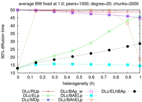
equal to20 and a playout delay of 50 (once again other numbers would not change the meaning and quality of the results). The outcome is shown in Figure 9, hich reports the 90-th percentile and show that BAELp is still the better performing algorithm. The reduced neighbourhood size seems to badly affect ELp when the heterogeneity of the system is high (hence, the performance of ELhBAp are also affected), and the BAhELp curve is now quite near to the second group of schedulers because the playout delay limits the upper bound of the chunk diffusion time to50 (of course, this results in a high number of lost chunks).
To check if these results depend on the bandwidth distribution scenario, the same experiment has been repeated in the uniform scenario, and the results are shown in Figure 10. Although all the values are generally higher than the values in Figure 9, the results are consistent and show that the relative performance of the various schedulers do not change. The comparison of these two figures indicates that highly inhomoge-neous scenario (in a uniform scenario we can have all bandwidths vaslues, while in the 3-class one only specific values are allowed) are harder to address. This is also a hint that even slow time-variability, not addressed in this contribution, may have an impact too.
In the next set of experiments, theB = 1 assumption has been removed, comparing the behaviour of the schedulers when the average upload bandwidth is increased. Fig-ure 11 reports the variation of the 90-th percentile of the chunk diffusion time with the average bandwidth. The simulation is based on a 3-class scenario withh = 0.5,
10 15 20 25 30 35 40 45 50 0 0.1 0.2 0.3 0.4 0.5 0.6 0.7 0.8 0.9 1 90% diffusion time heterogeneity (h)
average BW fixed at 1.0; peers=1000; degree=20; chunks=2000
DLc/RUp DLc/ELp DLc/MDp DLc/BAp_w DLc/BAELp DLc/BAhELp DLc/ELhBAp
Figure 9: 3-class scenario with neighborhood size 20 and playout delay 50: 90-th percentile of the diffusion delay as a function of the inhomogeneity factorh.
bourhood size20 and playout delay 50. Again, BAELp looks like the best performing algorithm (clearly, when the average bandwidth increases too much the differences be-tween the various algorithms become more difficult to notice). The same experiment has been repeated in the uniform scenario (withH = 0.8) and the results are reported in Figure 12. Again, the results are consistent with the 3-class scenario and BAELp is the best-performing algorithm.
Finally, we explore the ability of the various schedulers to cope with peers that do not participate to the stream distribution. In this “free-riders” scenario the neighbor-hood size must be increased, otherwise the system results fragile: we set it to 100 peer. Figure 13 reports the 90-th percentile of the chunk transmission delay as a function of the fraction of peers that do not participate to the distribution (free riders, having up-load bandwidth equal to0). Note that some curves (the ones relative to the ELp, RUp, MDp, and ELhBAp schedulers) stop at15% of free riders, because with higher frac-tions of free riders such schedulers are not able to properly diffuse the stream. Again, this experiment shows how BAELp outperforms all the other schedulers (more simu-lations in the free-riders scenario have been performed, and they confirmed the results of this experiment).
10 15 20 25 30 35 40 45 50 0 0.2 0.4 0.6 0.8 1 90% diffusion time heterogeneity (H)
average BW=1.0; peers=1000; degree=20; chunks=2000
DLc/RUp DLc/ELp DLc/MDp DLc/BAp_w DLc/BAELp DLc/BAhELp DLc/ELhBAp
Figure 10: Uniform scenario with neighborhood size 20 and playout delay 50: 90-th percentile of the diffusion delay as a function of the inhomogeneity factorh.
7
Related Work
The literature on p2P streaming is now so vast that a simple listing would require pages, starting from the commercial systems like PPlive and UUSee. However this paper deals with a specific, well identified problem: robust and performant schedulers in mesh-based unstructured systems. Here the literature shrinks quite a bit and restricting the analysis to distributed systems reduces it even more.
For the case of a homogeneous full mesh overlay (with upload bandwidth equal to 1 for all peers), the generic (i.e., valid for any scheduler) lower bound of (⌈log2(N )⌉ + 1)T is well known. [5] proved that such a lower bound can be reached in a stream-ing scenario by showstream-ing the existence of a centralised scheduler that achieves it. (a similar proof, developed for a file dissemination scenario, can be found in [7]). Re-cently, it has been proved that the theoretical lower bound can also be reached by using distributed schedulers, based on a chunk-first strategy (LUc/ELp and DLc/ELp) [1]. While the previous works focus on deterministic bounds for the diffusion times, some other works studied the asymptotic properties of distributed gossipping algorithms [8], or probabilistic bounds for specific well known algorithms [2] (in particular, it has been shown that the combination of random peer selection and LUc achieves asymptotically good delays if the upload bandwidths are larger than1).
Heterogeneous scenarios have also been considered [4, 5, 2, 6], but only few of such works (namely, [4, 5]) explicitly used bandwidth information in peer scheduling.
0 5 10 15 20 25 30 1 1.5 2 2.5 3 90% diffusion time average BW
3-class, h=0.5; peers=1000; degree=20; chunks=2000 DLc/RUp DLc/ELp DLc/MDp DLc/BAp_w DLc/BAELp DLc/BAhELp DLc/ELhBAp
Figure 11: 3-class scenario withh = 0.5, neighborhood size 20 and playout delay 50: 90-th percentile of the diffusion delay as a function of the average bandwidthB.
Moreover, most of the previous works only considered few possible scenarios, whereas in this paper 3 different kinds of scenarios (3-class, uniform, and free-riders) have been considered and the proposed algorithm, BAELp, appears to perform better than the other algorithms in all the considered cases.
8
Conclusions and Future Work
This paper compared a large number of scheduling strategies for P2P streaming sys-tems in presence of network heterogeneity (peers having different upload bandwidths) and considering different conditions and scenarios. Since none of the existing peer scheduling algorithms seems to perform well in all the conditions, a new peer schedul-ing algorithm, named BAELp, has been developed and compared with the other ones.
BAELp outperforms all the other scheduling algorithms in a large number of dif-ferent conditions and scenarios (in all the ones that have been tested): for example, in homogeneous networks BAELp is equivalent to ELp, which is optimal, and even in highly-heterogeneous networks it performs better than other bandwidth aware sched-ulers. This peer scheduler seems also the only one able to cope with the presence of free riders, namely peers that fro any reason cannot contribute to uploading chunks and sustaining the stream.
0 5 10 15 20 25 30 1 1.5 2 2.5 3 90% diffusion time average BW
uniform, H=0.8; peers=1000; degree=20; chunks=2000 DLc/RUp DLc/ELp DLc/MDp DLc/BAp_w DLc/BAELp DLc/BAhELp DLc/ELhBAp
Figure 12: Uniform scenario withh = 0.8, neighborhood size 20 and playout delay 50: 90-th percentile of the diffusion delay as a function of the average bandwidthB.
formed, and some of its theoretical properties will be analysed. Moreover, when using a DLc/BAELp scheduler there are two parameters that can be tuned: the amount of deadline postponing for DLc and the bandwidth weightw for BAELp. In this paper, the algorithm has been empirically tuned, but a more detailed analysis of the effects of the two parameters is needed. In particular, the optimal values might depend on the network conditions; in this case, some kind of self-adaptation of the scheduling parameters (based on a feedback loop) will be developed.
References
[1] Luca Abeni, Csaba Kiraly, and Renato Lo Cigno. On the optimal scheduling of streaming applications in unstructured meshes. In Networking 09, Aachen, DE, May 2009. Springer.
[2] Thomas Bonald, Laurent Massouli´e, Fabien Mathieu, Diego Perino, and Andrew Twigg. Epidemic live streaming: optimal performance trade-offs. In Zhen Liu, Vishal Misra, and Prashant J. Shenoy, editors, SIGMETRICS, pages 325–336, Annapolis, Maryland, USA, June 2008. ACM.
[3] M. Castro, P. Druschel, A.-M. Kermarrec, A. Nandi, A. Rowstron, and A. Singh. Splitstream: high-bandwidth multicast in cooperative environments. In
0 5 10 15 20 25 30 35 40 45 50 0 0.1 0.2 0.3 0.4 0.5 0.6 0.7 0.8 0.9 90% diffusion time
ratio of freeriders (inhomogeneous) average BW fixed at 1.0, low BW fixed at 0
peers=1000; degree=100; chunks=2000 DLc/RUp DLc/ELp DLc/MDp DLc/BAp_w DLc/BAELp DLc/BAhELp DLc/ELhBAp
Figure 13: Free Riders scenario,B = 1, neighborhood size 100 and playout delay 50: 90-th percentile of the diffusion delay as a fraction of the free riders.
ings of the nineteenth ACM symposium on Operating systems principles (SOSP 03), pages 298–313, New York, NY, USA, 2003. ACM.
[4] A.P. Couto da Silva, E. Leonardi, M. Mellia, and M. Meo. A bandwidth-aware scheduling strategy for p2p-tv systems. In Proceedings of the 8th
Interna-tional Conference on Peer-to-Peer Computing 2008 (P2P’08), Aachen,
Septem-ber 2008.
[5] Yong Liu. On the minimum delay peer-to-peer video streaming: how realtime can it be? In MULTIMEDIA ’07: Proceedings of the 15th international conference
on Multimedia, pages 127–136, Augsburg, Germany, September 2007. ACM.
[6] Laurent Massoulie, Andrew Twigg, Christos Gkantsidis, and Pablo Rodriguez. Randomized decentralized broadcasting algorithms. In 26th IEEE International
Conference on Computer Communications (INFOCOM 2007), May 2007.
[7] Jochen Mundinger, Richard Weber, and Gideon Weiss. Optimal scheduling of peer-to-peer file dissemination. J. of Scheduling, 11(2):105–120, 2008.
[8] Sujay Sanghavi, Bruce Hajek, and Laurent Massouli´e. Gossiping with multiple messages. In Proceedings of IEEE INFOCOM 2007, pages 2135–2143, Anchor-age, Alaska, USA, May 2007.
[9] S. Voulgaris, M. Jelasity, and M. Van Steen. A robust and scalable peer-to-peer gossiping protocol. In The Second International Workshop on Agents and
Peer-to-Peer Computing (AP2PC). Springer, 2003.
[10] Y.-H. Chu, S. G. Rao, and H. Zang. A case for end system multicast. In ACM