A Design Procedure for Sum and Difference Patterns by Means of Reactive Sorting Algorithm

UNIVERSITY

OF TRENTO

DIPARTIMENTO DI INGEGNERIA E SCIENZA DELL’INFORMAZIONE

38123 Povo – Trento (Italy), Via Sommarive 14

http://www.disi.unitn.it

A DESIGN PROCEDURE FOR SUM AND DIFFERENCE PATTERNS

BY MEANS OF REACTIVE SORTING ALGORITHMS

L. Manica, P. Rocca, D. Franceschini, and A. Massa

January 2011

A DESIGN PROCEDURE FOR SUM AND DIFFERENCE PATTERNS BY MEANS OF

REACTIVE SORTING ALGORITHMS

L. Manica, P. Rocca, D. Franceschini, and A. Massa

Department of Information and Communication Technologies, University of Trento, Via Sommarive 14, 38050 Trento – Italy Tel. +39 0461 882057, Fax +39 0461 882093

Email: andrea.massa@ing.unitn.it, {luca.manica, paolo.rocca, davide.franceschini} @dit.unitn.it

ABSTRACT

A new approach for the synthesis of both sum and difference antenna pattern is proposed. The approach allows to obtain an optimal sum pattern and a sub-optimal difference pattern through the search of a minimal cost path inside an incomplete binary tree.

1. INTRODUCTION

A monopulse radar tracker is a device in which the angular position of a target is obtained through the use of two beams antenna [1]. These beams are the sum and the difference pattern and they can be generated by an antenna array. These patterns have to satisfy some constrains as narrow beam-width, low side lobe level (SLL), high directivity, etc… . By a proper choice of the excitation coefficients, computed using analytical methods as described in [2] for the sum mode and in [3] for the difference mode, the optimal sum and difference patterns can be generated. Unfortunately this solution leads to two independent feed networks with generally unacceptable costs, circuit complexity, and interference phenomena. Therefore, it is necessary to find a compromise solution with a simpler feed network but leading to sub-optimal sum and difference patterns. The most common way to solve such a problem [4] consists in generating an optimal sum pattern and a sub-optimal difference pattern by means of sub-arraying. Consequently, the unknowns of the problem are the element grouping (sub-array configuration) and values of the weights to be associated at each sub-array such that the sub-optimal pattern is as close as possible to the optimal one.

Several approaches for defining the sub-array configuration and the weights have been proposed. In particular, the strategy proposed by McNamara [4] finds the solution considering a particular sub-array configuration and obtains the weights solving an over-determined system of linear equations. The approach presented by Ares in [5] allows to find the weights for a given sub-array configuration by minimizing a cost function through the simulated annealing. These two approaches present the inconvenient that it is impossible to know “a priori” which is the sub-array configuration that will bring to the best solution.

Such drawback has been solved by Lopez [6]. A simultaneous optimization of the sub-array configurations and the weights is performed through the minimization by a GA of a cost function related with the SLL of the generated beam. A similar solution has been proposed by Caorsi [7]. Also in this case, a joint optimization of both the sub-array configurations and weights is performed by using a Differential Evolution (DE). Although these approaches overcome the problem of the choice of the sub-array configuration, they usually require large computational resources because of the wide solution space.

In order to overcome such a problem, the present work is aimed at introducing a new technique able to efficiently deal with large arrays. The approach is based on the key-observation that an optimal array grouping can be obtained considering elements with similar properties. Moreover, neglecting a set of non allowed or equivalent sub-array configurations, the solution space can be reduced without any loss of information and the candidate configurations can be generated by means of a non-complete binary tree. The solution of the problem is successively found associating a cost to each complete path inside the tree and choosing the configuration with minimal cost.

Toward this aim, an algorithm for a fast search of the solution is also presented. It optimizes only the positions of special elements, called border elements, inside the sub-array configurations which are suitable candidates to change sub-array of membership.

This work is organized as follows. In Sect. 2 the problem is mathematically formulated and then in Sect. 3 some numerical example are presented and discussed. Finally, in Sect. 4 some conclusions will be drawn.

2. MATHEMATICAL FORMULATION

Let us consider a linear uniform array of N=2M elements and assume that the sum pattern is generated by a symmetric real excitations set A=

{

a_m=a_−mm=1,...,M

}

[8] and the difference pattern is obtained by using an anti-symmetric real

excitations set B=

{

b_m =−b_−mm=1,...,M

}

[9]. Thanks to such symmetry properties only half of the array can be taken

in account.

In order to obtain the best performances, the optimal sum excitations coefficients A

{

m m M

}

opt

,..., 1 ; =

= α and the

optimal difference excitations ones B

{

m m M

opt

,..., 1 ; =

= β

}

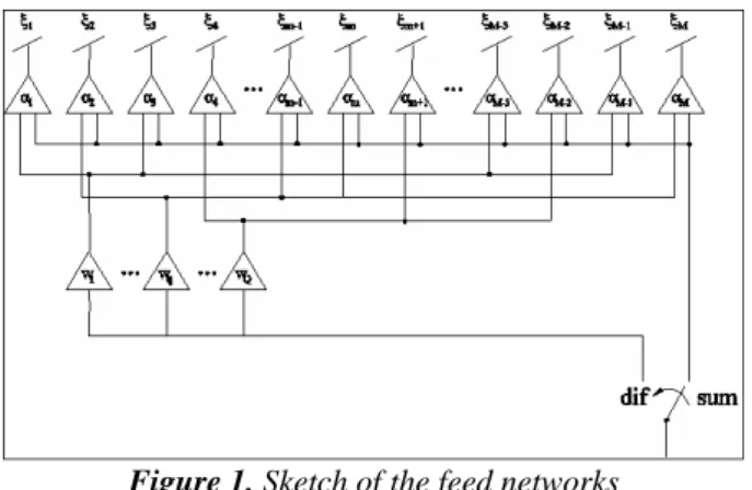
can be computed according to the procedure described in [2] and in [3], respectively. Unfortunately this approach needs the implementation of two independent feed networks.

Figure 1. Sketch of the feed networks

To overcome such a drawback, the sub-array technique is widely adopted to obtain simpler feed networks able to generate the optimal sum pattern, but only a sub-optimal difference pattern. Accordingly, the array elements are suitable grouped in Q sub-arrays (Fig. 1) and each sub-array configuration can be mathematically described [7] by the vector:

{

; m 1,...,M

}

,

m c

C= = (1)

where is the sub-array index of the mth element. Moreover, a weight is associated for each sub-array so that the difference pattern is generated by the following excitations

[

Q cm∈1,

]

w

q

{

; m 1,...,M q 1,...,Q

}

, m mq w m b B= = α = = (2)

where is the weight associated to the mth array element belonging to the qth sub-array. Thus, the goal of the problem is to determine a sub-array configuration

q mq w

w =

C and a set of Q weights such that the difference pattern generated by B is as close as possible to the optimal one.

2.1. Construction of the Solution Tree

The space of the sub-array configurations can be reduced without any lost of information through some observations. First, only the configurations in which there is at least one element in each sub-array are considered (allowed configurations). Moreover, it can be observed that some configurations are equivalent since it is possible to obtain one from the others just using a different numbering for the same . Clearly, it is possible to consider just one configuration for each set of equivalent ones.

m

c

After reducing the solution space and before representing it by means of a binary tree, a sorting operation of the array elements is performed. Toward this end, let us introduce a set V of known real parameters , each one associated to an element of the array. The parameters are sorted to obtain a list of real elements where

. Such a choice allows us to obtain a solution closer the optimal one.

m v

{

l ;m 1,...,M

}

, L= _m = M i l li+1≤ i, =0,...,

Then, all the possible solutions are represented through a non-complete binary tree of depth M, called solution tree. Referring to Fig. 2, each complete path of the tree represents a possible sub-array configuration C and the positive integer q inside the nodes at the mth level indicates that lm is a member of the qth array.

Figure 2. Solution tree

2.2. Definition of the Metric

In order to find the best configuration, it is necessary to quantify the closeness of a trial solution to the optimal one. Toward this end, a cost is associated to each path of the tree:

, 1 ∑ = − = Ψ M m m d m v (3)

where are the known parameters and the are the elements of the trial solution. Two different definitions of the optimal parameters have been used in the Gain Sorting algorithm (GS) and in the Residual Error algorithm (RES), respectively.

m v dm , ,..., 1 ,m M m v =

In the GS algorithm the parameters v_mare called optimal gains and are defined as: , ,..., 1 ;m M m m m v = = α β (4)

being α_m and β_m the optimal excitation coefficients. The parameters are called computed gains and can be computed directly as:

m d , ,..., 1 ; 1 1 M m M m cmq M m m v q m c m d = = ∑ = = ∑ δ δ (5) being _{c q} m

δ the Kronecker delta ( _{c q}=1

m

δ if cm = , q δcmq=0 otherwise). The weights are then computed as:

m mq d

w = (6)

, ,..., 1 ;m M m m m m v = − = β β α (7) Substituting (7) and (2) in (3) the cost function can be rewritten as:

. 1 ∑ = − = Ψ M m _m m b m β β (8)

Eq. 8 represents the normalized difference between the optimal difference excitations Bopt _{and the effective excitations}

set B. The value of the weights wq are in this case computed using the equivalence between (3) and (8) and according

to the following expression:

(

)

. 1 1 1 ⎟⎟ ⎠ ⎞ ⎜⎜ ⎝ ⎛ − − =

∑

∑

= = m m M m q c M m m m q c q m m v d w β α δ δ (9)

2.3. Fast Search of the Solution

Notwithstanding the reduction of the solution space, an exhaustive search is prohibitive, in terms of computational time, for large arrays (M>>Q). In order to overcome such drawback, it can be observed that only some elements are candidate to change sub-array of membership without violating the condition of a sub-array configuration with sorted . These elements are called border elements. In particular is a border element if and/or are members of different sub-arrays.

m

l

m

l lm lm−1 lm+1

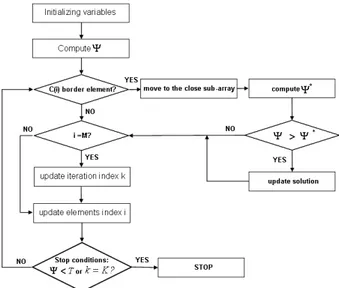
Starting from these considerations, the algorithm summarized in the flow chart of Fig. 3 has been developed. Firstly, a random trial solution is generated, and its cost is computed. Then, the solution is searched for scanning all the elements of the list. If is a border element, then its possible membership to the closest sub-array is checked by considering a new solution with aggregates to it.

i

l

i

l

Figure 3. Flow chart of the algorithm for the fast research of the solution.

The cost function of the new solution is computed and if it is lower than that of the previous solution, the sub-array configuration is updated. According to this strategy, the whole vector C can be scanned iteratively until the cost function is higher than a given threshold or k=K.

As far as the computational costs are concerned, the number of operations needed for sorting the elements is O(M*log(M)) and the evaluations of the cost function used to find the solution follow the law O(M2_).

3. NUMERICAL SIMULATIONS

The proposed approach has been validated through a set of representative numerical simulations. The first test case concerns with an array of N=2M=20 elements spaced by λ/2 with the optimal sum pattern corresponding to a Villenueve pattern [8] with n=4 (for which SLL=-25[dB]) and the optimal difference pattern corresponding to a Zolotarev pattern [3] with n=4 and ε=3 (for which SLL=-25[dB]). The excitation coefficients and the parameters involved in the simulation are indicated in Tab. 1.

m αm βm vm - RES vm– GS 1 1.0000 0.1739 4.7521 0.1739 2 0.9760 0.4961 0.9671 0.5083 3 0.9271 0.7550 0.2279 0.8144 4 0.8542 0.9272 -0.0788 1.0855 5 0.7616 1.0000 -0.2384 1.3130 6 0.6583 0.9659 -0.3184 1.4672 7 0.5567 0.8401 -0.3373 1.5091 8 0.4692 0.6833 -0.3134 1.4563 9 0.4057 0.5464 -0.2575 1.3468 10 0.3726 0.3610 0.0323 0.9688

Table 1. Excitation coefficients and optimal parameters for a linear array of N=20 elements.

The sub-optimal pattern obtained for Q=3 is compared with the patterns generated by McNamara [4] (analytical approach) and by Lopez [6] . The results are shown in Fig. 4.

Figure 4. Comparison between GS – [4] – [6] and the optimal one [3] for Q=3.

The pattern generated by the GS in a computational time of 0.0347[sec] shows a good approximation of the optimal pattern till |θ|<600_{. Moreover, for values of |θ| exceeding this range the SLL is always lower than -20[dB]. The pattern}

obtained with the GS algorithm is comparable with that obtained in [4] and with narrower beam-width with respect to [6].

Using the same excitation coefficients for the sum and the difference mode, the pattern generated using the RES algorithm with Q=6 is compared with the pattern generated in [7] and with the optimal one. The results are shown in Fig. 5. The pattern generated by the RES shows a very good approximation of the optimal pattern. In particular, the SLL doesn’t exceed -27[dB] and the envelope is similar to the optimal one. The RES pattern presents better performances in comparison to [7]’s approach in term of SLL. Moreover, the result has been calculated in 0.05841[sec]. The last test case concerns with a linear array of N=2M=100 elements spaced by λ/2. The optimal sum pattern excitations corresponds to a Taylor pattern [9] with n=12 (SLL=-35[dB]) and the optimal difference pattern has been chosen as that generated by the Lopez approach [6] for Q=4. The result is shown in Fig. 6.

Figure 5. Comparison between RES - [7] and the optimal one [3] for Q=6.

The RES algorithm approximates very well a generic reference pattern and the SLL doesn’t exceed -30[dB]. The computation time is still very reasonable ( 0.1164[sec] for the RES algorithm and 0.1827[sec] for the GS algorithm). These results allow us to extend the field of application of the approach in all the synthesis problems where the generation of two different patterns is needed and the excitation coefficients are known.

Figure 6. RES and GS pattern for N=100 and Q=4 - Optimal difference pattern [6].

4. CONCLUSIONS

A new approach to optimize the compromise between the circuit complexity and the sub-optimal difference pattern has been described. The strategy allows the reduction of the configurations space and the generation of all the possible solutions by means of a non-complete binary tree. Each complete path is characterized by a cost and the best solution can be selected considering the minimal cost path. The exhaustive search of the best solution has been avoided observing that just some elements inside a sub-array configuration are candidate to change sub-array of membership. The proposed strategy has shown similar performances in comparison to the analytical approach presented in [4] and the GA optimization presented in [7] for small sub-array. Moreover, since the solution is obtained by means of a fast algorithm, the approach seems to be potentially a good strategy for dealing with large arrays.

5. REFERENCES

1. Skolnik, I. Merrill, Radar Handbook, McGraw-Hill, 1990.

2. T. T. Taylor, “Design of a line-source antennas for narrow beam-width and low side lobes.,” Trans. IRE, vol. AP-3, pp. 16-28, Jan. 1955.

3. D. A. McNamara, “Discrete n-distributions for difference patterns,” Electron. Lett., vol.22, no.6, pp.303-304, June 1986.

4. D. A. McNamara, “Synthesis of sub-arrayed monopulse linear arrays trough matching of independently optimum sum and difference excitations,” IEE Proc. H, vol. 135, no.5, pp. 371-364, Oct. 1988.

5. F. Ares, S. R. Rengarajan, J. A. Rodriguez, and E. Moreno, “Optimal Compromise Among Sum and Difference Patterns Trough Sub-Arraying,” IEEE Antennas and Propagations Symposium, pp. 1142-1145, July 1996.

6. P. Lopez, J. A. Rodriguez, F. Ares and E. Moreno, “Subarray weighting for Difference Patterns of Monopulse Antennas: Joint Optimization of Subarray Configurations and Weights,” IEEE Trans. Antennas Propagat., vol. 49, no.11, pp.1606-1608, Nov. 2001.

7. S. Caorsi, A. Massa, M. Pastorino, and A. Randazzo, “Optimization of the Difference Patterns for Monopulse Antennas by a Hybrid Real/Integer-Coded Differential Evolution Method,” IEEE Trans. Antennas Propagat., vol. 53, no.1, pp.372-376, Jan. 2005.

8. A. T. Villenueve, “Taylor Patterns for Discrete Arrays,” IEEE Trans. Antennas Propagat., AP-32, pp. 1089-1093, May 1984.