CHINA’S INCOME DISTRIBUTION AND TRADE

1 / 148

UNIVERSITÀ DEGLI STUDI DI MACERATA

DIPARTIMENTO DI ECONOMIA E DIRITTO

CORSO DI DOTTORATO DI RICERCA IN

METODI QUANTITATIVI PER LA POLITICA ECONOMICA

CICLO xxx

TITOLO DELLA TESI

CHINA’S INCOME DISTRIBUTION AND TRADE

RELATORE DOTTORANDO

Chiar.mo Prof. Elisabetta Croci Angelini Dott. LIU Yang

COORDINATORE

Chiar.mo Prof. Maurizio Ciaschini

2 / 148

LIU YANG_CHINA‘S INCOME DISTRIBUTION AND TRADE

Abstract

After 1978 economic reform, China‘s economy has been keeping booming growth. Meanwhile, China‘s income inequality has been growing rapidly. China‘s Gini Coefficient was around 0.30 in 1978, it has reached over 0.40 the international alertness line since 2000, and then hit the peak 0.49 in 2009. In recent years, the Gini coefficient has been decreasing, and went down to 0.46 in 2015. It shows an incomplete reversed U shape curve. Moreover, the China‘s import and export trade volume have risen from 0.038 trillion dollar in 1980 to 3.95 trillion in 2015, an annual growth rate of about 14%. In the most recent years the value of import and export went down slightly. It seems that there is a relationship between China‘s Gini Coefficient and the value of import and export.

Based on previous studies this research illustrated the influence mechanism of effect of income inequality on import and export at provincial level. And static and dynamic regressions model were used to test the effect of income inequality on import and export. The results are significant at the 99% level, and suggest income inequality within provinces (measured by Gini coefficient) brings about trade, which means that when the Gini coefficient increases also import-export increase. Meanwhile, income inequality between provinces (measured by Theil elements) restrains import and export.

This dissertation calculated multidimensional poverty by fuzzy set at provincial level, and found there is some correlation between multidimensional poverty and import-export.

KEY WORDS: CHINA, INCOME INEQUALITY, IMPORT AND EXPORT, MULTIDIMENSIONAL POVERTY

3 / 148

Index

1.3.2.1 Why inequality is important? ... 8

1.3.2.2 What is income inequality? ... 9

1.3.2.3 Levels, dimensions and variables related ... 10

1.3.2.4 Charting income inequality... 11

1.3.2.5 Measurements ... 13

I. Gini Coefficient ... 14

II. Dispersion Ratio Measures ... 16

III. Theil index and General Entropy measures... 17

IV. The Robin Hood Index ... 18

V. Atkinson‘s inequality measure ... 19

VI. Range ... 20

VII. Summary ... 20

1.3.3 Poverty ... 21

1.3.3.1 Poverty income standards ... 22

1.3.3.2 The poverty line ... 22

1.3.4 Multidimensional poverty ... 22

2. State of the Art... 25

2.1. The evolution of China’s income inequality ... 25

2.1.1. Current status on income inequality in China ... 25

2.1.2. China’s income distribution policy evolution ... 42

2.1.2.1. The dualistic structure system of urban and rural areas ... 42

2.1.2.2. 'Egalitarianism' ... 42

2.1.2.3. Breaking down 'Egalitarianism'... 43

2.1.2.4. Distribution according to work, efficiency and equity... 44

2.1.2.5. For more equality ... 45

2.1.2.6. Conclusion ... 46

2.1.3. Discussion... 47

2.1.3.1. The inflection point of Kuznets curve. ... 47

2.1.3.2. The Lewis turning point ... 49

2.1.3.3. The future income distribution reform ... 51

2.2. China’s poverty evolution and multidimensional poverty studies... 51

2.2.1. China's poverty evolution ... 51

2.2.2. Multidimensional Poverty in China ... 57

2.3. The evolution of China’s import-export ... 58

3. Literature Review ... 62

3.1. China’s income inequality ... 62

3.1.1. Measurement ... 62

3.1.2. Contribution Factors ... 64

3.1.3. Consequence ... 67

3.1.4. Conclusion ... 68

3.2. The effect of import-export on income inequality and China’s cases ... 68

Conclusion... 71

4 / 148

3.3.1. The effect of income inequality on import ... 71

3.3.2. The effect of income inequality on export ... 74

3.4. The effect of China’s multidimensional poverty to import-export ... 76

4. Empirical Studies ... 78

4.1. The effect of China’s income inequality to import-export ... 79

4.1.1. Influence Mechanism and Modeling ... 79

4.1.2. Data and Variables ... 80

4.1.3. Methodology ... 82

4.1.4. The first results ... 82

4.1.5. General Results to solve the Endogeneity Problem ... 86

Conclusion ... 90

4.2. The effect of multidimensional poverty to import-export ... 90

4.2.1. Influence Mechanism and Modeling ... 91

4.2.2. Data and process ... 92

4.2.3. Methodology ... 95

4.2.3.1. Fuzzy sets ... 95

4.2.3.2. MPI ... 96

4.2.4. Results ... 96

4.2.4.1. Multidimensional poverty based on personal data ... 96

4.2.4.2. Multidimensional poverty based on household data ... 97

4.2.4.3. Multidimensional poverty based on province data ... 98

4.2.4.4. Comparing multidimensional poverty data and import-export data ... 101

Conclusion ... 103

5. Conclusion ... 104

References ... 106

6. Appendix ... 113

6.1. CHIP (Chinese Household Income Project Survey) ... 113

6.2. Tables ... 114

5 / 148

1. Introduction 1.1 Background

Since the late 1970s China‘s economic growth has been an economic miracle in the world. China‘s GDP were 3,678,700 million CNY in 1978. After economic reform 1978 (reform and open up; reform and openness), China‘s economy has been keeping booming growth rates. By 2016, China‘s GDP increased to 743,585,500 million CNY. The normal GDP annual growth reached 15%; even she passed through the financial crisis of 2007–2008. According to the WDI database, by 2010 China‘s GDP 5.93 billion USD (40.143 billion CNY) had surpassed that of Japan and became the second largest economy after the U.S. However, it was 149.54 billion USD (251.77 billion CNY) and ranked 13th in the world in 1978. According of data published by NBSC (National Bureau of Statistics of China) the Chinese Total Value of Imports and Exports have risen from 20,640 USD million (35,500 million CNY) in 1978 to 3,685,557 USD million (24,338,646 million CNY) in 2016, while the peak 4,301,527 USD million (26,424,177 million CNY) was reached in 2014. The annual growth of total value of trade is 14.6% from 1978 to 2016. China‘s has been the second largest importer and exporter in the world. Beside GDP and Imports and Exports, there has been growth in infrastructure, reserves, foreign direct investment, and development assistance.

But, at the same time, there has been growth in spatial divergence, and corruption, an underclass of migrant workers, environmental pollution, carbon emissions, and inequality. China only took three decades and brought her Gini coefficient to a very high 0.5 from a very low level 0.2.

China had adopted planned economy and equalitarianism over a long period since new China was established in 1949. Since 1978, China broke down equalitarianism and carried out a series of reforms to economic transition from planned economy to market economy. The inequality of China rose like trapped bird gets freedom. China‘s Gini coefficient took just twelve years to rise to 0.3 from 0.2. And ten years later it reached 0.4. The 0.4 is the international alertness line, according to the United Nation‘s definition, and a coefficient of 0.4-0.5 means high income disparity. More surprise was that in 2008 it approached 0.5 only eight years later. Even a report (China Household Finance Survey, 2013)1 indicated China‘s household income inequality hit 0.6. Just 30 years after economic reform, China‘s inequality creased two levels from ―relative equality‖ to ―high income disparity‖ and jumped over the relatively reasonable level (0.3-0.4). In these ten years, the forth ten years form 1978 economic reform, China‘s Gini coefficient has been keeping at level of 0.4 according to NBSC. We could simply say the Gini coefficient almost reached the summit.

1

China Household Finance Survey, 2013, China Household Income Inequality Report (zhongguo jiating shouru chaju baogao), Southwestern University of Finance and Economics

6 / 148

Figure 1.1 - 1. The values of import-export evolution

Data Sources：National Bureau of Statistics of China

Figure 1.1 - 2. The China‘s Gini coefficient evolution

Data Sources：National Bureau of Statistics of China and World Bank (WDI)

What the ―Opening‖ has brought to China since 1978? We can say they are high level of value of trade and inequality. If we draw a diagram with the values of import-export and Gini coefficients,

7 / 148

we could find their trends look like similar. Since the economic reform 1978, the Gini coefficient has been rising rapidly. The values of import-export increased at the beginning slowly, and then faster around 1992, much more speedily since China's accession into WTO in 2001 as Figure 1.1 - 1 and Figure 1.1 -2 show. We know their growths were synchronous, but their growth rates were different. Intuitively speaking, it seems there are relationships between import-export and income inequality.

According to the classical trade theories, trade improves income distribution, in other words, it reduces income inequality. Neoclassical international trade theory, the New Trade Theory and the new classical international trade theories, have the similar opinion on the relationship between trade and income distribution. The pattern of trade and inequality evolutions above, tell another story: trade did not improve income distribution in China. Both are growths, even synchronous. All the theories we mentioned above are unfit to explain the Chinese case. Considering how the theories, which are invalid, explained the relationship between trade and income distribution on aspects of Supply, it means the effect comes from trade to income distribution. The relationship goes probably in another way. We may say we could figure it out from opposite view, the Demand side: the effect of income distribution on trade.

The current theories on Demand side to explain relationship between trade and income distribution are not explicit about the influential mechanism. Linder (1961)2 made the first try on it. The subsequent studies on the relationship between trade and income distribution on Demand side are all based on Linder‘s theory. This dissertation takes Demand side as theoretical justification, and explains the effect of income distribution on trade. We try and explain the China‘s case and endeavor in filling up the theoretical gap.

1.2 Contribution

For a long time, most studies on the relationship between income distribution and trade have been promoted on supply-side, which mean how trade affects income distribution. Few studies have started in the opposite, from the perspective of demand, which mean income distribution affects trade. Many researches were developed ignoring the demand-side model, but this type of analysis is undoubtedly important. This dissertation examines trade from the perspective of demand, expands the research horizon on the correlation between trade and income distribution, and further enriches the theory of demand-side. In the demand-side theory, only per capita income is used as the representative of demand. However, the total demand is not only affected by the average income level, but also affected by income distribution. This dissertation introduces income distribution indicators into the trade model to closely connect them two.

2

8 / 148

This dissertation is meaningful also in reality. At present, the income distribution disparity in China has been widening year by year, while trade has continued to prosper and China has got a Trade Surplus for a long time. Does the expansion of the income distribution gap have an impact on trade? China has become the second largest importer country. Is income distribution an important factor in China's imports? China is currently the world's largest exporter. What is the relationship between income distribution and export? Has China‘s trade continued to have a long-term surplus, and is it related to income distribution? Answering these questions is important for China at this stage and for other developing countries, too.

1.3 Conception 1.3.1 Income

Income is defined by NBSC in urban areas as ―disposable income‖ including employee income (wages, salaries, and other compensation), self-employment income, property income, and transfer income from public and private sources, net of taxes and fees. The NBSC defined rural income as ―net income3_{‖ including cash income from employment, and household business and production} activities such as farming, as well as the monetary values of self-produced consumption, net of production costs, taxes and fees, depreciation of productive assets, and net private transfers. The measurement consists primarily of cash income from various sources; imputed rents on owner-occupied housing are not included. Moreover, income in-kind is not fully captured.

Khan et al. (1992)4 pointed out two shortcomings of the NBSC‘s income measures. One is the exclusion of imputed rent of owner-occupied housing. Another is the understatement of consumption subsidies, mostly to urban households. In the past, consumption subsidies arose due to the provision of low-priced consumer goods and subsidized rental housing under the planned economy. Later, since 1978 economic reform, the consumption subsidies have been gradually eliminated, as well as the urban rental housing, but not completely.

In the light of Khan et al. (1992) considerations, we have two kinds of Income; one referred to ―Income NBSC‖, another as ―CHIP income‖, which is equal to NBSC income plus imputed rents on owner-occupied housing plus implicit subsidies on subsidized public urban rental housing. In this dissertation we take ―NBSC income" when we explore income inequality and trade, while we use ―CHIP income‖ when we explore multidimensional poverty.

1.3.2 Income Inequality

1.3.2.1 Why inequality is important?

3

National Bureau of Statistics of China (2008), Zhongguo Nongcun Zhuhu Diaocha Nianjian 2008 (China Yearbook of Rural Household Survey 2008), Beijing: China Statistics Press (Zhongguo Tongji Chubanshe)

4

Khan, A.R., K. Griffin, C.Riskin, and R.Zhao (1992), “Household Income and Its Distribution in China,” China Quarterly, no. 132, 1029-1061.

9 / 148

Inequality is an important value in modern societies. Irrespective of economics, philosophy, religion, culture, ideology, people care about inequality. Income inequality has always been viewed as closely related to conflict. In the introduction of his celebrated book On Income Inequality, Amartya K. Sen (1973)5 asserts that ―the relation between inequality and rebellion is indeed a close one.‖ The more serious inequality involves poverty, which makes the study of inequality more meaningful. Since economic inequality makes a material difference, at some choices on material object some people could choose, while the others could not have the same set of choices. However, resources are generally limited. For a given level of average income, education, capital, asset, land ownership etc., increased inequality of these characteristics will almost always imply higher levels of both absolute and relative deprivation in these dimensions.6

Inequality matters from poverty to opportunities and rights. People always fight for their own opportunities and rights. If the degree of inequality is acceptable by the majority of the population, the fighting may reduce the inequality within the society, if not, the conflict comes up. An unstable social environment leads to a more difficult economic growth because of inequality7. Therefore, the inequality matters for economic growth at the macro level. So, in economics, widening inequality has significant implications for growth and macroeconomic stability; it can concentrate political and decision making power in the hands of a few, lead to a suboptimal use of human resources, cause investment-reducing political and economic instability, and raise crisis risk.8

The economic inequality is divided in wealth inequality and income inequality. Wealth inequality is a stock concept of economic inequality, while income inequality is a flow concept of economic inequality.

1.3.2.2 What is income inequality?

Income is usually defined over household or individual disposable income in a particular year. It consists of earnings, self-employment and capital income and public cash transfers; income taxes and social security contributions paid by households are deducted. The income of the household is attributed to each of its members, with an adjustment to reflect differences in needs for households of different sizes. This is why the concept of equivalent income has been introduced.9 Income inequality is the unequal distribution of household or individual income across the various participants in an economy.10

5

Sen, Amartya K. 1973. On Economic Inequality. Oxford: Clarendon Press, Chapter 1 6

McKay, A.(2002). Defining and Measuring Inequality.Overseas Development Institute and University of Nottingham. Briefing Paper No 1 (1 of 3). March 2002.

7

Alesina, A. and Perotti P. (1996). Income Distribution.Political Instability and Investment, EER 40(6):1203-1229. 8

Era Dabla-Norris, Kalpana Kochhar, and Nujin Suphaphiphat.(2015).Causes and Consequences of Income Inequality : A Global Perspective. International Monetary Fund, June 15, P6

9

OECD (2017), Income inequality (indicator). doi: 10.1787/459aa7f1-en (Accessed on 12 November 2017) https://data.oecd.org/inequality/income-inequality.htm

10

10 / 148

The economic inequality people often talk about refers to three aspects, income, wealth and consumption. Wealth is an economic stock indicator, while income and consumption are economic flow indicators.

Income inequality is the most commonly cited measure, primarily because the data on it is the most comprehensive.11 Income is a relatively straightforward matter of wages and compensation. However, wealth is more mercurial. It can be a physical asset like a car, house, or land. But it can also be a stock or bond or other financial asset.12 Income decides your standard of living, but wealth gives you control over the shape and future course of the economy. Generally, wealth is the most unevenly distributed of the three, income the second, consumption the least. Wealth is an important metric since it can be inherited, unlike income. So it is a suitable variable to study Hierarchical solidification. Meanwhile, income inequality is a more suitable variable than wealth inequality to study well-being and social stability.

Consumption inequality, though harder to measure, provides a better proxy of social welfare. This is because people‘s living standards depend upon the amount of goods and services they consume, rather than upon how much valuable possession they are having. Consumption is also thought to have diminishing marginal utility, because of The Law of Diminishing Marginal Propensity to Consume, a poorer person will value an additional unit of consumption more than the richer person.

1.3.2.3 Levels, dimensions and variables related

Considering income inequality, one should think about levels, dimensions and variables related. Generally speaking, income inequality could be described at different aggregation levels which often result in different geographical areas. If we talk about decomposition income inequality, the Theil index could achieve it.

By measurement the Theil index, Income inequality can be decomposed at different levels of geographical aggregations. At the national level it can be decomposed into within-subgroup, between subgroup, and overlapping components. In a similar way at the international level it can be decomposed into within-country, between-country, and overlapping components. In the measurement of world income inequality, it is desirable that the unit of analysis is the citizens of the world rather than countries.

11

A three-headed hydra, the economist, Jul 16th 2014, 10:33 BY Z.G. | LONDON, https://www.economist.com/blogs/freeexchange/2014/07/measuring-inequality 12

Jeff Spross, Wealth inequality is even worse than income inequality,

11 / 148

Representative individual based micro data is preferable.13 The dimensions, generally speaking at the micro-level, involve gender, education, residency, occupation and so on, and refer to the demographic aspects of the population. Meanwhile, many of the economic variables related to income inequality are available at the macro-level, imbalanced regional growth, consumption, issues on the labor market, aging, inflation, social crime, happiness, financial structure, savings, taxation, public policy, marketization, economic development, credit, international trade, education, industry, social behavior, free trade, etc.

1.3.2.4 Charting income inequality

The diagrammatic form is a visual expression. If we talk about income inequality, we could chart income inequality by Pen‘s parade and Lorenz curve.

Pen's Parade, or the Income Parade, is a concept described in a 1971 book published by Dutch economist Jan Pen describing income distribution. The parade is defined as a succession of every person in the economy, with their height proportional to their income, and ordered from lowest to highest. The Pen's description of what the spectator would see is a parade with dwarves at the beginning, and then some unbelievable giants at the very end.14

The original context of the parade is the United Kingdom, and the duration is one hour. The parade is used by economists as a graphical representation of income inequality because it's a form of quantile function and it is considered useful when comparing two different areas or periods.15

Figure 1.3 - 1. Pen‘s parade, ranking persons by their incomes

13

Almas Heshmati. (2004).Inequalities and Their Measurement. IZA Discussion Paper No. 1219 14

Crook, Clive (September 2006). "The Height of Inequality". The Atlantic. Retrieved 28 May 2015. 15

12 / 148

Figure 1.3 - 2. Comparing two Pen‘s parade curves

This picture (Figure 1.3 - 2) is Pen‘s parade (quantile function)16 for expenditure per capita, Vietnam, 1993 and 1998. X axis shows the cumulative percentage of individuals, from poor to rich, by 100 units. If Y axis shows the income, the solid line represents more inequality than the dashed line.

The Lorenz curve is a graphical representation of the distribution, such as, income or wealth. It was developed by Max O. Lorenz in 1905 for representing inequality of income or of the wealth distribution. Lorenz curve, sorts the population from poorest to richest, and shows the cumulative proportion of the population on the horizontal axis and the cumulative proportion of income (or expenditure) on the vertical axis. On the graph, a straight diagonal line represents perfect equality of income distribution; the Lorenz curve lies beneath it, showing the reality of income distribution. The area comprised between the straight line and the curved line represents the amount of inequality of income distribution. Lorenz curve A therefore represents lower inequality vis-à-vis Lorenz curve B.

Figure 1.3 - 3. Lorenz Curve

16

Haughton, Jonathan; Khandker, Shahidur R.. 2009. Handbook on poverty and inequality. Washington, DC: World Bank.P109, Pen’s parade (quantile function) for expenditure per capita, Vietnam, 1993 and 1998

13 / 148

1.3.2.5 Measurements

Four criteria for inequality measurement:17 make income inequality assessment universal.

1) Anonymity principle (sometimes called the symmetry principle), which says that it does not matter who receives the income. Permutations of incomes among people should not matter for inequality judgments. This means that we can always arrange the income distribution of n people so that y1≤y2≤…≤yn, where y is income. If the prime minister trades his income with

one of yours, income inequality should not change.

2) Population principle, which says that cloning the entire population and their incomes should not change overall inequality. According to this principle, population size does not matter. All that matters are the proportions of the population that earn different levels of income.

3) Relative income principle, which says that only relative incomes and not the absolute levels of these incomes matter. For example, think of an income distribution over two people: the first having half income with respect to the second, e.g. (500, 1000). This principle means that the same inequality level should be found as with (2000, 4000), and therefore it would be the same regardless of the currency the incomes are denominated in.

4) The Dalton principle (also known as ―Pigou-Dalton transfer principle‖): Let (y1,y2,…,yn) be

an income distribution and consider two incomes yi and yj, with yi ≤ yj. A transfer of income

from the ―not richer‖ individual to the ―not poorer‖ individual will be called a regressive

17

Debraj Ray, development economics, Oxford University Press

0.00 0.20 0.40 0.60 0.80 1.00 0% 10% 20% 30% 40% 50% 60% 70% 80% 90% 100% C u m u la ti ve In co m e

Cumulative population from lowest to highest income

Lorenz Curve

Lorenz curve B

Lorenz curve A

14 / 148

transfer and makes inequality higher. The Dalton principle states that if one income distribution can be generated from another via a sequence of regressive transfers, then the original distribution is more equal than the other. Formally, we say that i satisfies the Dalton principle if and only if for every income distribution, i(y1 ,...,yi ,...,yj ,...,yn) ＜

i(y1 ,...,yi-δ,...,yi+δ,..., yn), for every positive number δ.

I. Gini Coefficient

The Gini coefficient is based on the comparison of cumulative proportions of the population against cumulative proportions of income they receive.18 It is a measure of the deviation of the distribution of income among individuals or households within a country from a perfectly equal distribution.19 It is defined as half the average of all pairwise absolute deviations between people, relative to the mean income. It ranges between 0 in the case of perfect equality and 1 in the case of perfect inequality. The Gini‘s main limitation is that it is not easily decomposable or additive. Also, it does not respond in the same way to income transfers between people in opposite tails of the income distribution as it does to transfer in the middle of the distribution. Furthermore, the same Gini coefficient can represent very different income distributions.

Figure 1.3 - 4. The Gini Coefficient related to Lorenz Curve

The Gini coefficient can be related to the Lorenz curve: it is calculated by the ratio of area A over area A+B. On the graph earlier, the Gini is 0 if there is total equality and 1 if there is total inequality.

18

Income inequality, OECD Data, https://data.oecd.org/inequality/income-inequality.htm 19

Income Gini coefficient, Human Development Reports,United Nations Development Programme, http://hdr.undp.org/en/content/income-gini-coefficient 0% 20% 40% 60% 80% 100% 0% 10% 20% 30% 40% 50% 60% 70% 80% 90% 100% C u m u la ti ve In co m e

Cumulative population from lowest to highest income

The Gini Coefficient related to Lorenz Curve

A

15 / 148

𝐺𝑖𝑛𝑖 =_{area (A + B)} area A

Calculate the Gini coefficient with formula:

Gini coefficient = ∑ ∑ |𝑦𝑖− 𝑦𝑗| 𝑛 𝑗=1 𝑛 𝑖=1 2𝑛(𝑛 − 1)𝑦̅

Where yi and yj are individual incomes or consumptions with a mean ofy, and n is the total

number of observations for both individual and households.

The advantage of Gini coefficient is that it is easy to understand, in the light of the Lorenz curve. However, the first disadvantage, the Gini coefficient is not additive. The aggregate Gini for the total population is not equal to the sum of the Gini coefficients for its subgroups. The second disadvantage, the coefficient is sensitive to changes in the distribution, irrespective of whether they take place at the top, the middle or the bottom of the distribution (any transfer of income between two individuals has an impact, irrespective of whether it occurs among the rich or among the poor). The third, Gini coefficient gives equal weight to those at the bottom and those at the top of the distribution.

There are a plenty of studies about the calculation and decomposition of Gini coefficient The related study could be found by Chakravarty (1990)20, Cowell (2000)21, Atkinson (1970a)22, Shorrocks (1984)23, Shi Li(1999,24 200225), Zongsheng Chen(2002)26, Yonghong Cheng(200627, 200828), Chengwu Jin(2007)29, Zuguang Hu(2004)30, Guanghua Wan(2004)31, Jing Dong, Zinai

20

Chakravarty, S. R.(1990).Ethical Social Index Numbers[M]. New York: Springer Verlag.P53 21

Cowell, F. A.(2011). Measuring Inequality [M]. Oxford: Oxford University Press.P39 22

Atkinson, A. B.(1970).On the measurement of inequality[J].Journal of Economic Theory, 1970a(2):P244-263 23

Shorrocks, A. F.(1984).Inequality Decomposition by Population Subgroups[J]. Econometrica, 1984(52):P1369-86 24

Li, Shi. and Zhao, Renwei.(1999). A study on income distribution of Chinese Residents 2 (Zhongguo Jumin Shouru Fenpei Zaiyanjiu)[J] Economic Research Journal,1999(4):3-17

25

Li, Shi. (2002).Further Explanation Of The Gini Coefficient Estimation And Decomposition: A Reply To Professor Chen Zongsheng 'S Comments (Dui Jinni Xishu Gusuan Yu Fenjie De Jinyibu Shuoming – Dui Chen Zongsheng Jiaoshou Pinglun De Zaidafu)[J]. Economic Research Journal,2002(5):P84-7

26

Chen, Zongsheng. (2002). A Suggestion On The Calculation Method Of The Overall Gini Coefficient - A Re-Comment For Researcher Shi Li's "Reply"(Guanyu Zongti Jini Xishu Jisuan Fangfa De Yige Jianyi – Dui Li Shi Yanjiuyuan<Dafu>De Zaipinglun) [J]. Economic Research Journal, 2002(5):P81-7

27

Cheng, Yonghong.(2006).Calculation And Decomposition Of The Overall Gini Coefficient In Dual Economies (Eryuan Jingji Zhong Chengxiang Hunhe Jini Xishu De Jisuan Yu Fenjie) [J]. Economic Research Journal, 2006(1):P109-120

28

Cheng, Yonghong.(2008).A New Decomposition Of Gini Coefficient By Population Subgroups (Jini Xishu Zuqun Fenjie Xinfangfa Yanjiu: Cong Chengxiang Eryazu Dao Duoyazu)[J]. Economic Research Journal. 2008(8) :P124-44. 29

Jin, Chengwu.(2007). Gini Coefficient for Discrete income data in Vector-Matrix Forms and Related issues(Lisan Fenbu Shouru Shuju Jini Xishu De Juzhen Xiangliang Xingshi Ji Xiangguan Wenti)[J]. Economic Research

Journal,2007(4):P149-58. 30

Hu, Zuguang.(2004). A Study Of The Best Theoretical Value Of Gini Coefficient And Its Concise Calculation Formula(Jini Xishu Lilun Zuijiazhi Jiqi Jianyi Jisuan Gongshi Yanjiu) [J]. Economic Research Journal. 2004(9):P60-9 . 31

Wan, Guanghua.(2004). Measurement and Decomposition of Income Distribution: A evluation for

16 / 148

Li(2004)32, Hu Li(2005)33, Xingjian Hong(2008)34, Jinfeng Zhang, Peiguo Yu(2006)35 et al.

II. Dispersion Ratio Measures

The dispersion ratios measure the ―distance‖ between two groups in the distribution of income. Typically, they measure the average income of the richest x% divided by the average income of the poorest x%. There are different alternatives, the most frequently used are for deciles and quintiles. A decile is a group containing 10% of the total population ranked according to their individual income from poorer to richer.

Decile ratio = average income of top group i average income of bottom group j

Group i and group j can be defined as deciles (1/10), quintiles (1/5), quartiles (1/4), percentiles (1/100), etc.

The advantage of the decile ratio is readily understandable. Comparing to the top group and bottom group, to some extent, it shows the inequality according to the ratio. The higher the ratio is, the more inequality is observed.

The disadvantage is that the value of decile ratio is very much vulnerable to extreme values and outliers, especially in case of estimates from small samples. In addition, its meaning is mathematical rather than economic, because it is not derived from principles about equity.

The other common indicators following this measure are:

Quintile ratio, the 20:20 ratio compares how much richer the top 20% of people are, compared to the bottom 20%.36 If it is more inequality in a group the first quintile or last quintile, its decile ratio should be more sensitive. Quintile ratio is better to see the whole.

P90/P50 of the upper bound value of the ninth decile to the median income, it shows the distance between the upper and the median. The less the ratio is, the more equality is. It is mainly to study the upper group income.

2004(1):P64-9. 32

Dong, Jing. And Li, Zinai.(2004). Revise The Urban-Rural Weighting Method And Application: Estimating The China's National Gini Coefficient By The Rural-Urban Gini Coefficients(Xiuzheng Chengxiang Jiaquanfa Jiqi Yingyong – You Nongcun He Chengzhen Jinni Xishu Tuisuan Quanguo Jinni Xishu) [J]. The Journal of Quantitative & Technical Economics,2004(5):P120-3.

33

Li, Hu.(2005).A Research On Gini Coefficient Decomposition Analysis(Guanyu Jinni Xishu Fenjie Fenxi De Taolun) [J]. The Journal of Quantitative & Technical Economics,2005(3):P127-35.

34

Hong, Xingjian.(2008). A New Subgroup Decomposition Formula for Gini Coefficient: Urban - rural

Decomposition of China 's Gini Coefficient (Yige Xinde Jinni Xishu Ziqun Fenjie Gongshi – Jian Lun Zhongguo Zongti Jinni Xishu De Chengxiang Fenjie)[J]. China Economic Quarterly, 2008(10):P307-24.

35

Zhang, Jinfeng. and Yu, peiguo. (2006). Calculate the Gini Coefficient by Group: A matrix decomposition method (An Renqun Fenzu Jisuan Quanguo Jinni Xishu: Yizhong Juzhen Fenjie Fangfa) [J], Statistics and Decision, 2006(12):P142-3.

36

17 / 148

P50/P10 of median income to the upper bound value of the first decile,37 it shows the distance between the lowest and the median. The less the ratio is, the more equality is. It is mainly to study the lowest group income.

- Palma Ratio

The Palma ratio, named after Gabriel Palma (2011) is the ratio of the income share of the top 10% to that of the bottom 40%. In more equal societies this ratio will be one or below, meaning that the top 10% does not receive a larger share of national income than the bottom 40%. The Palma ratio addresses the Gini coefficient's over-sensitivity to changes in the middle of the distribution and insensitivity to changes at the top and bottom.38,39

III. Theil index and General Entropy measures

The values of the General Entropy (GE) class of measures vary between zero (perfect equality) and infinity (or one, if normalized). A key feature of these measures is that they are fully decomposable, i.e. inequality may be broken down by population groups or income sources or using other dimensions, which can prove useful for policy makers. Another key feature is that researchers can choose a parameter α that assigns a weight to distances between incomes in different parts of the income distribution. For lower values of α, the measure is more sensitive to changes in the lower tail of the distribution and, for higher values, it is more sensitive to changes that affect the upper tail (Atkinson and Bourguignon, 2015)40. The most common values for α are 0, 1, and 2. When α=0, the index is called ―Theil‘s L‖ or the ―mean log deviation‖ measure. When α=1, the index is called ―Theil‘s T‖ index or, more commonly, ―Theil index‖. When α=2, the index is called ―coefficient of variation‖. Similarly to the Gini coefficient, when income redistribution happens, change in the indices depends on the level of individual incomes involved in the redistribution and the population size (Bellù, 2006)41.

For a population of N "agents" each with characteristic x, the situation may be represented by the list xi (i=1,...,N) where xi is the characteristic of agent i. If the characteristic is income, then xi is

the income of agent i. The Theil index is defined as42:

𝑇𝑇= 1 𝑁∑ 𝑥𝑖 𝜇𝑙𝑛 ( 𝑥𝑖 𝜇) 𝑁 𝑖=1 37 https://data.oecd.org/inequality/income-inequality.htm 38

Alex Cobham, Palma vs Gini: Measuring post-2015 inequality,Center For Global Development,4/5/13 http://www.cgdev.org/blog/palma-vs-gini-measuring-post-2015-inequality

39

How is Economic Inequality Defined? The equality trust

https://www.equalitytrust.org.uk/how-economic-inequality-defined 40

Anthony, B. Atkinson and François,Bourguignon.(2015).Handbook of Income Distribution 41

Bellù, L. G., and Liberati, P. (2006), ‘Describing Income Inequality: Theil Index and Entropy Class Indexes’, Food and Agriculture Organization of the United Nations

42

18 / 148

Where μ is the mean income:

𝜇 =_𝑁1∑ 𝑥𝑖

𝑁

𝑖=1

Because of decomposable characteristics, Theil index could be represented by,

Tt = Tb+ Tw

Where Tt is total Theil index, Tb is Theil index between group, Tw is Theil index within group.

𝑇𝑏= ∑ 𝑦𝑘𝑙𝑛 ( 𝑦𝑘 𝑁𝑘 𝑁⁄ ) 𝐾 𝑘=1 𝑇𝑤= ∑ 𝑦𝑘( ∑ 𝑦𝑖 𝑦𝑘 𝑖∈𝑔𝑘 𝑙𝑛𝑦𝑖 𝑦𝑘₁⁄ 𝑁𝑘 ⁄ ) 𝐾 𝑘=1

k is the number of groups, denotes N agents divided by k groups. The group called gk, (k=1,…,k), Nk is the number of agents in group gk and yk is the income share of group k over the total income. yi is the income share of agent i over the total income.

While the General Entropy is defined as43:

𝐺𝐸(𝛼) = 1 𝛼2_{− 𝛼}[ 1 𝑁∑ ( 𝑥𝑖 𝜇) 𝛼 − 1] 𝑁 𝑖=1

Where α is the weight given to distances between incomes at different parts of the income distribution.

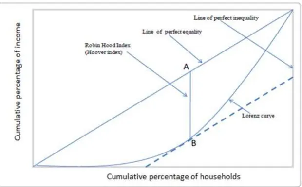
IV. The Robin Hood Index

Conceptually, this is a simple measurement of inequality used in income metrics. It is equal to the portion of the total community income that would have to be redistributed (taken from the richer half of the population and given to the poorer half) for the society to live in perfect equality. The Robin Hood index44 is based on the Lorenz Curve and is closely tied to the better known inequality measure the Gini coefficient, which is also based on the Lorenz curve. In other words, the Robin Hood index is the proportion of money which would need to transfer from the rich to the poor to achieve equality.

43

Feng, Xinguang.And Zhang, Xiaojing.(2005). Measuring And Decomposing Of Regional Inequality Based On Generalized Entropy Index:1978-2003(Jiyu Guangyishang Zhishu De Diqu Chaju Cedu Yu Fenjie:1978-2003), Statistics & Information Forum, Vol.20 No.4,July,2005

44

Edgar Malone Hoover jr. (1936) The Measurement of Industrial Localization, Review of Economics and Statistics, 18, No. 162–71

19 / 148 H = 1/2 ∑ | 𝐸𝑖 𝐸𝑡𝑜𝑡𝑎𝑙− 𝐴𝑖 𝐴𝑡𝑜𝑡𝑎𝑙| 𝑁 𝑖=1

Where Ei is the income of quintile i and Ai is the amount of earners in quintile i, while Etotal is the sum of incomes and Atotal is the sum of all earners.

The Robin Hood index is equivalent to the maximum vertical distance between the Lorenz curve, or the cumulative portion of the total income held below a certain income percentile, and the Perfect Equality Line, that is the 45 degree line of equal incomes.

Figure 1.3 - 5. the value of Robin Hood Index equal the distance of AB

V. Atkinson’s inequality measure

Atkinson‘s inequality measure (or Atkinson‘s index) is the most popular welfare-based measure of inequality. It presents the percentage of total income that a given society would have to forego in order to have more equal shares of income between its citizens. This measure depends on the degree of society aversion to inequality (a theoretical parameter decided by the researcher), where a higher value entails greater social utility or willingness by individuals to accept smaller incomes in exchange for a more equal distribution. An important feature of the Atkinson index is that it can be decomposed into within-and between-group inequality. Moreover, unlike other indices, it can provide welfare implications of alternative policies and allows the researcher to include some normative content to the analysis (Bellù, 2006).

20 / 148

Atkinson noted inequality cannot be measured without introducing social judgments45 as the formula showing below,

𝐴𝜀= 1 − [ 1 𝑛∑ [ 𝑦𝑖 𝜇] 1−𝜀 𝑛 𝑖=1 ] 1 1−𝜀

Aε𝐴𝜀 is Atkinson‘s index. yi is income of individual or group i, n is the number of sample, ε is

sensitivity parameter, also called ―inequality aversion parameter‖, 0<ε<+∞ where 0 means that the researcher is indifferent about the nature of the income distribution, while infinity means the researcher is concerned only with the income position of the very lowest income group.

In practice, ε values of 0.5, 1, 1.5 or 2 are used; the higher the value, the more sensitive the Atkinson index becomes to inequalities at the bottom of the income distribution.

VI. Range

The Range (or called ―The Relative Range‖ is imputed by Range over a given value like mean) is the common statistical measures of dispersion for a distribution in general. It is useful measures in the context of income. The range is defined as the absolute difference between the highest and the lowest income levels divided by the mean income:

RGE =(x max – x min)/µ

Where the arithmetic mean income is µ=1/n∑ni=1 yi

The method is easy to understand and calculate. Another advantage is this method is not affected by inflation. However, it is very sensitive to extreme observations, while it ignores all but two of the observations.

VII. Summary

The Range and Dispersion Ratio Measures satisfy the first three criteria, and are easy to understand and calculate, but violate the Pigou-Daltion principle by ignoring the distribution inside the range. If we have not enough data, they are still proper measurements. The Robin Hood Index violates the Pigou-Daltion principle, too. For instance, when transfer happens between high income observation and low income observation comparing to mean income, the Robin Hood Index changes. Otherwise, when transfer happens within higher income observation, or within lower income observations, the Robin Hood Index will not change.

The Gini coefficient, Theil‘s inequality measures and Atkinson‘s index satisfy all four criteria conditions.46 The Gini Coefficient generally regarded as gold standard in economic work. It is attractive intuitive interpretation. Also, it allows direct comparison between units with different

45

Atkinson AB. The economics of inequality. Oxford: Clarendon Press, 1975. p.47. 46

Almas Heshmati, Inequalities and Their Measurement, MTT Economic Research and IZA Bonn, July 2004, Discussion Paper No. 1219

21 / 148

size populations. It incorporates all data. Just for this reason, it requires comprehensive individual level data and imputed with a more sophisticated method. A major limitation of Lorenz curves is that since when two Lorenz curves intersect we can not say which distribution is more unequal.

Theil‘s T Statistic lacks an intuitive picture and involves more than a simple difference or ratio. It is comparatively mathematically complex measure. Nonetheless, it has several properties that make it a superior inequality measure. Theil‘s T Statistic can incorporate group-level data and is particularly effective at parsing effects in hierarchical data sets. Theil's T allows the researcher to parse inequality into within group and between group components. There is a limited should be considered if compare populations with different size that Thei‘s T cannot directly compare populations with different sizes or group structures

Considering to the inability of the Gini framework to give different parts of the income spectrum varying weights, the Atkinson index allows for varying sensitivity to inequalities in different parts of the income distribution. Atkinson‘s index can be decomposed, but the sum is not equal to between add within.

1.3.3 Poverty

Income is an important proxy variable to measure poverty, is an important tool to achieve poverty alleviation, but cannot fully reflect the real poverty situation. To this end, some other variables are added to measure poverty. Based on Amartya Sen's capability approach, Alkire and Foster (2007)47 constructed a multidimensional poverty index to fully reflect the multi-dimensional deprivation of the poor. The multidimensional poverty index includes important indicators that reflect environmental poverty and asset poverty. Income variable and multi-dimensional poverty methods are valuable to measure poverty, monitor poverty and formulate anti-poverty policy.

The understanding of poverty is an evolving process that progresses with the development of human society. The definition of poverty is also deepening and enriching. Initially, people's awareness of poverty was largely confined of avoiding hunger and malnutrition. In 1901, the British scholar Benjamin Seebohm Rowntree (1901)48 began to use income to define British poverty. In 1981, the World Bank began to calculate the consumption and income poverty of the developing countries. In 1990, based on the capability approach of the Amartya Sen, the Human Development Index (HDI) first time is presented in the Human Development Report by the United Nations Development Programme, and defined poverty on the perspective of human development. In 2010, based on Sabina Alkire's measurement, multi-dimensional poverty index (MPI) is presented in the Human Development Report by UNDP, and expanded the measurement of

47

Alkire,S;Foster,J.E Counting and multidimensional poverty measures.[OPHI Working Paper 7,]2007 48

22 / 148

poverty. So far, we can classify the widely used criteria for measuring poverty: income variable and multidimensional poverty.

1.3.3.1 Poverty income standards

Britain is the first country to develop poverty income standards. The British scholar Benjamin Seebohm Rowntree, in his 1901 book, The Study of "Poverty: A Study of Town Life", based on the money budget required for the "shopping basket" of "the minimum needed to maintain physical strength", and estimate the poverty line of York City. For a family of six people, the lowest food budget for the week is 15 shillings. With some housing, clothing, fuel and other expenditure, he arrived at a poverty line of twenty-six shillings for a family of six that implied a poverty rate of almost 10 percent in York. (Kanbur R., and L., Squire 1999, p. 3)49 This is the first assessment in terms of food and non-food goods sub-divided in two parts that defines poverty in a monetary variable.

1.3.3.2 The poverty line

The World Bank (1990)50 introduced the dollar-a-day international poverty line. The World Bank's definition of poverty is "deprivation of welfare", in which welfare is primarily concerned with whether individuals or families have sufficient resources to meet their basic needs. The World Bank has collected the poverty lines of 33 countries (including developing and developed countries), and using the 33 national poverty line data to identify poverty lines that can be used for global poverty comparisons. The World Bank adjusted the monetary unit of the poverty line in these countries in accordance with the purchasing power parity PPP in 1985 to forecast the poverty line, and found that the monthly consumption of the poorest six countries (Indonesia, Bangladesh, Nepal, Kenya, Tanzania, Morocco), was around $ 31/person. Accordingly, the World Bank has set a poverty line of $1/day. After that a new set of PPPs was published in 1993, the line changed to $1.08 per day. PPPs were revised again in 2005, and the line was correspondingly upped to $1.25. The World Bank set $ 1.25 per day poverty line by estimating the average of the 15 least developed countries' poverty lines. The World Bank‘s international poverty line has been raised to $1.90 per day51 since 2015.

1.3.4 Multidimensional poverty

In 1987, Hagenaars52 introduced leisure in the study of poverty, and constructed the first multidimensional poverty index from the two dimensions of income and leisure, making poverty

49

Kanbur, R., & Squire, L. (1999). The Evolution of Thinking about Poverty: Exploring the Interactions. Working Papers from Cornell University, Department of Applied Economics and Management. No 127697,P3

50

World Development Report 1990 51

The international poverty line has just been raised to $1.90 a day, but global poverty is basically unchanged. How is that even possible?

http://blogs.worldbank.org/developmenttalk/international-poverty-line-has-just-been-raised-190-day-global-pov erty-basically-unchanged-how-even

52

23 / 148

research not only at the income level, but also focusing on factors other than income. Since 1997, the United Nations has adopted the Human Poverty Index (HPI) to measure multidimensional poverty. The HPI concentrates on the deprivation in the three essential elements of human life already reflected in the HDI: longevity, knowledge and a decent standard of living.

Amartya Sen (2003, 2004)53, studied poverty up to the level of personal welfare then rose to the level of social development. He sees development as a process of people's enjoyment of substantive freedoms from basic viability, including avoiding hunger and malnutrition, living older, engaging in economic transactions or participating in political activities. Sen's method of defining poverty is called capability approach. Amartya Sen points out that the core of multidimensional poverty is that not only income poverty, but also poverty encompasses several dimensions some of which can be regarded as objective (such as drinking water, roads, sanitation and other objective indicators) and other subjective feelings of poverty. Sen's theory of multi-dimensional poverty has been put forward by academics, governments and international agencies.

The Multidimensional Poverty Index (MPI) was presented in the 2011 Human Development Report which is based on Sen's theory and is classified among the various measures of poverty, which replaced Human Poverty Index (HPI). The difference is that HPI is summed up by the national macro-level data, reflecting the deprivation of health, education and living standards, and MPI can measure from the micro level, such as the individual or family level, not only to reflect the incidence of deprivation, but also to reflect the depth of deprivation of poverty, to carry out various aspects of decomposition, to understand the relative proportion of poverty MPI support personal or family level of micro-data, gender age, regional dimensions and other aspects of decomposition. HPI focuses on three dimensions, life expectancy, knowledge and standard of living, and three indicators for developing countries (probability of not surviving till age 40, adult illiteracy rate, and means average of population with sustainable access to an improved water source and children under weight for age), and four indicators for developed countries (probability of not surviving till age of 60, adult who doesn‘t have functional literacy skills, population below income poverty line and rate of long term unemployment). MPI also forces 3 dimensions, health, education, and living standards, with 10 indicators (child mortality, nutrition, years of schooling, school attendance, cooking fuel, toilet, water, electricity, floor, assets). Comparing to HPI, MPI has some advantages: more indicators than HPI could be better and less susceptible to bias; identifying the most vulnerable and poorest among the population; revealing spatial and temporal, inter and intra nation and regional variations; effective allocation of resources by targeting greatest

53

Sen,A. A Decade of Human Development [J].Journal of Human Development,2003,17-23. Sen,A.Elements of a theory of human rights, Philosophy and Public Affairs[J].2004,315-356. Sen,A. Dialogue Capabilities, Lists, and Public Reason: Continuing the Conversation[J].Feminist Economics,2004,77-80.

24 / 148

intensity of poverty; monitoring impacts of policy intervention for eradication programs. However, MPI needs much more data than HPI for calculating.

25 / 148

2. State of the Art

2.1. The evolution of China’s income inequality 2.1.1. Current status on income inequality in China

This part is described by levels, including national, regional, provincial, urban, rural, urban-rural and industrial. For well-understanding it is presented by income and Gini coefficient two indicators.

I. National level

China’s income inequality (Gini coefficient-Based)

The World Bank published China‘s Gini Coefficients which was 0.29 in 1981, and then ten years later it went up to 0.32 in 1990, and after another decade it became 0.42 in 2002. China‘ Gini coefficient has broken through 0.40 (since 2002, or even since 200054,) which is a serious figure in economics named the ―international alertness line‖. The data published by the NBSC indicated China‘s Gini coefficient was between 0.473 - 0.491 from 2003 to 2012. The Gini coefficient was 0.473 in 2013, while it was 0.469 in 2014.

Table 2.1 - 1. China‘s Gini coefficients (1981 – 2010)

Year 1981 1984 1987 1990 1993 1996 1999 2002 2005 2008 2010

Gini 29.11 27.69 29.85 32.43 35.5 35.7 39.23 42.59 42.48 42.63 42.06

Source: World Bank

Table 2.1 - 2. China‘s Gini coefficients (2003 – 2016)

Year 2003 2004 2005 2006 2007 2008 2009

Gini 0.479 0.473 0.485 0.487 0.484 0.491 0.490

Year 2010 2011 2012 2013 2014 2015 2016

Gini 0.481 0.477 0.474 0.473 0.469 0.462 0.465

Source: National Bureau of Statistics of China

Table 2.1 - 3. China‘s Gini coefficients (1978-2008)

year 1978 1979 1980 1981 1982 1983 1984 1985 Gini 0.31 0.305 0.322 0.297 0.269 0.263 0.264 0.242 year 1986 1987 1988 1989 1990 1991 1992 1993 Gini 0.305 0.309 0.319 0.348 0.341 0.358 0.377 0.407 year 1994 1995 1996 1997 1998 1999 2000 2001 54

Source: National Development and Reform Commission, Research Group of institute of social development, A Study on the Income Distribution Pattern of resident in China [J]. Economic Research

26 / 148

Gini 0.399 0.397 0.38 0.369 0.376 0.389 0.402 0.413

year 2002 2003 2004 2005 2006 2007 2008

Gini 0.44 0.45 0.451 0.452 0.453 0.455 0.457

Source: National Development and Reform Commission, Research Group of institute of social development, (2012) A Study on the Income Distribution Pattern of resident in China [J]. Economic Research Reference, 2012 (21)：32-82.P67

With other studies measurements, let‘s take a picture and have a look at China‘s Gini coefficient evolution according to different sources.

Figure 2.1 - 1. China‘s Gini coefficients evolution from 1978 to 2016

Source: World Bank, Ravallion and Chen (2007)55, World development indicators, World Income Inequality Database, Chinese Household Income Project, Lin et al.(2010)56, National Bureau of Statistics of China

That concludes the degree of income inequality in term of Gini in China. China‘s Gini goes stable nine years after economic reform, and then grows rapidly in 15 years from 0.298 in 1987 to 0.491 in 2008. After 2008, the Gini declines little by little and ends 0.465 in 2016. The whole shape goes like a half inverted U-shape, and it is expected a whole inverted U-shape eventually.

It has been over 0.40 international alert line since the beginning of 21th century, and it is still high, even though it has declined since 2008 up to 2016 with 5% decline from 0.491 to 0.465.

55

Ravallion, M., and S. Chen. 2007. China’s (Uneven) Progress against Poverty. Journal of Development Economics.82 (1). pp. 1–42.

56

Lin, T., J. Zhuang, D. Yarcia, and F. Lin. 2010. Decomposing Income Inequality: People’s Republic of China, 1990−2005. In J. Zhuang, ed. Poverty, Inequality, and Inclusive Growth in Asia: Measurement, Policy Issues, and Country Studies.Manila: ADB and London: Anthem Press

27 / 148

II. Regional level

Figure 2.1 - 2. Decile income by region 2013

Data source: CHIP 2013

The Chinese Household Income Project (CHIP) is a project developed by China Institute for Income Distribution to measure and estimates the distribution of personal income in both rural and urban areas of the People's Republic of China. The data were collected through a series of questionnaire-based interviews conducted in rural and urban areas. The sample covers half provinces and corresponds to half of the population of China. Based on the 2013 data, this dissertation ranked all income and got decile income by 3 regions (eastern, central and western). It is clear that income of eastern regions is more than that of the central regions, and that of western regions is less than that of central regions. At the first income decile (the poorest Chinese people), it covers 19% eastern population, 41% central and 40% western. At the last decile (the richest Chinese people), it covers 59% eastern population, 25% central and 16% western. It presents clearly how income distribution goes in these 3 regions.

III. Provincial level

China’s provincial inequality (GDP -Based)

Gross Domestic Product (GDP) is one of the most widely used measures of an economy‘s output or production. It is defined as the total value of goods and services produced within the geographic boundaries of a country‘s or an area‘s borders in a specific time period – monthly, quarterly or annually. Although it is not flawless, the GDP is the most accurate indication available for an

0% 10% 20% 30% 40% 50% 60% 70% 80% 90% 100% 1 2 3 4 5 6 7 8 9 10 western central eastern

28 / 148

economy's size.57 Referring to the population size and GDP as provincial income we also take per GDP to consider the provincial income inequality.

Figure 2.1 - 3. Gross Regional Product per capita (yuan) from 1993 to 2015 in China

Source: National Bureau of Statistics

The figure illustrates the GDP per capita from 1993 to 2015 at the provincial level in China. Considering the evolution of the curves through the years, the provinces GDP per capita apparently evolved yielding four classes in China on the basis of their per capita GDP.

In the class I: Beijing, Tianjin, Shanghai;

In the class II: Inner Mongolia, Liaoning , Jiangsu, Zhejiang , Fujian, Shandong, Guangdong; In the class III: Hebei, Shanxi, Jilin, Heilongjiang, Anhui, Jiangxi, Henan, Hubei, Hunan, Guangxi, Hainan, Chongqing, Sichuan, Shaanxi, Qinghai, Ningxia, Xinjiang;

In the class IV: Guizhou, Yunnan, The Tibet, Gansu.

Comparing the highest and lowest, the GDP per capita class 1 Tianjin is 3.98 times as much as class 4 Gansu in 2014, while class 1 Shanghai‘s was 8.96 times as much as class 4 Guizhou‘s in 1993. Therefore it does not seem that more inequality has taken place across provinces. However, if we set aside the population factor, the GDP of class 1 Guangdong 678,098.500 (million yuan) is 24.64 times as much as of class 3 Ningxia 27521 in 2015, while class 2 Guangdong‘s GDP was 34,692.800 (million yuan) and 92.72 times as much as class 4 Tibet‘s 374.200 (million yuan) in 1993.

57

Elvis Picardo, The GDP and its Importance,investopedia, August 2, 2016 - 5:34 PM EDT http://www.investopedia.com/articles/investing/121213/gdp-and-its-importance.asp

29 / 148

Otherwise, in these two classes, the biggest gap of per capita disposable income is 4.28 times as much as Shanghai 45,965.83 yuan compares Tibet 10,730.22 yuan in 2014.

It concludes the degree of income inequality in terms of per GDP in provinces in China. The province with higher per GDP is always the higher, the lower is always lower.

Figure 2.1 - 4. China‘s provinces GDP per capita, 2015

The same situation happens for the GDP. It is clearly divided in three or four classes. The top three always are Guangdong, Jiangsu and Shandong. At the bottom they are always Qinghai, Ningxia, Hainan and Tibet. The others are in the middle.

30 / 148

Source: National Bureau of Statistics

IV. Inter Urban

A. China’s income inequality (Income-Based): Per Capita Disposable Income of Urban Households

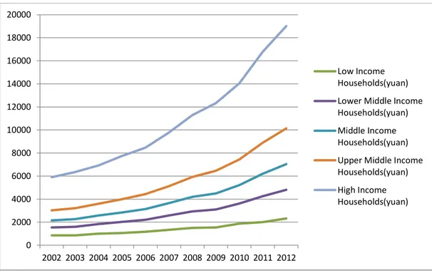
Figure 2.1 - 6. Per Capita Disposable Income of Urban Households decile (yuan) 2000-2012

Data Sources：National Bureau of Statistics of China

According to the Per Capita Disposable Income of Urban Households decile data from NBSC, Per Capita Disposable Income of Urban Households the lowest and the highest income households are 8,215.1 yuan and 63,824.2 yuan in 2012, while they were 2,408.6 yuan and 18,995.9 yuan in 2002.

31 / 148

The ratios between the highest and the lowest are around 7.8 in 2012 and 2002. However the others years, all ratios are above 7.8, while there are two peaks of about 9.18 times in 2005 and 2008. That means the pattern shows an inverted U-shape during the 11 years period between 2002 and 2012 (see figure 2.1 -7).

Figure 2.1 - 7. The ratio between the highest and the lowest decile of Per Capita Disposable Income of Urban Households 2002-2012

Table 2.1 - 4. Per Capita Disposable Income of Urban Households decile and quintile (yuan) 2002-2012 2002 2003 2004 2005 2006 2007 2008 2009 2010 2011 2012 1st 10% 2408.6 2590.2 2862.4 3134.9 3568.7 4210.1 4753.6 5253.2 5948.1 6876.1 8215.1 2nd 10% 3649.2 3970 4429.1 4885.3 5540.7 6504.6 7363.3 8162.1 9285.3 1067.2 1248.6 2nd 20% 4932 5377.3 6024.1 6710.6 7554.2 8900.5 10195.6 11243.6 12702.1 14498.3 16761.4 3rd 20% 6656.8 7278.8 8166.5 9190.1 10269.7 12042.3 13984.2 15399.9 17224 19544.9 22419.1 4th 20% 8869.5 9763.4 11050.9 12603.4 14049.2 16385.8 19254.1 21018 23188.9 26420 29813.7 9th 10% 11772.8 13123.1 14970.9 17202.9 19069 22233.6 26250.1 28386.5 31044 35579.2 39605.2 10th 10% 18995.9 21837.3 25377.2 28773.1 31967.3 36784.5 43613.8 46826.1 51431.6 58841.9 63824.2 Ratio 7.9 8.4 8.9 9.2 9.0 8.7 9.2 8.9 8.6 8.6 7.8

Per Capita Disposable Income of Urban Households 1st 10%: Lowest Income Households (first decile group) 2nd 10%: Low Income Households (second decile group)

2nd 20%: Lower Middle Income Households (second quintile group) 3rd 20%: Middle Income Households (third quintile group)

4th 20%: Upper Middle Income Households (fourth quintile group) 9th 10%: High Income Households (ninth decile group)

7.5 8 8.5 9 9.5 10 2002 2003 2004 2005 2006 2007 2008 2009 2010 2011 2012

Ratio between Urban Income highest 10% and

lowest 10%

32 / 148

10th 10%: Highest Income Households (tenth decile group) Ratio: ratio between highest 10% and lowest 10%

Data Sources：National Bureau of Statistics of China

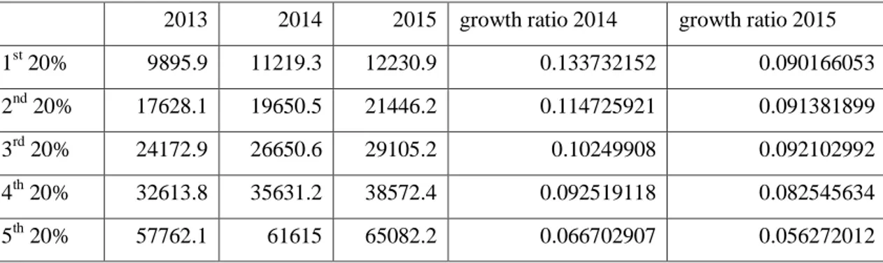
Since 2013, the survey method and index caliber of household income and living conditions were changed by National Bureau of Statistics because of the integration of urban and rural. The income definition is also changed, therefor we can not comparing them pre-2013 and post-2013. However, we found the income growth ratio was going down quickly, and the income growth ratio of low income group decreased quickly, but income growth ratio decreased slowly for the high income group. Since the high income group growth slow and the low income group growth slower, we can conclude the income inequality within urban was going wide since 2013.

Figure 2.1 - 8. Growth ratio of per capita disposable income of urban households by income quintile 2014-2015

Table 2.1 - 5. Per capita disposable income of urban households by income quintile

2013 2014 2015 growth ratio 2014 growth ratio 2015

1st 20% 9895.9 11219.3 12230.9 0.133732152 0.090166053

2nd 20% 17628.1 19650.5 21446.2 0.114725921 0.091381899

3rd 20% 24172.9 26650.6 29105.2 0.10249908 0.092102992

4th 20% 32613.8 35631.2 38572.4 0.092519118 0.082545634

5th 20% 57762.1 61615 65082.2 0.066702907 0.056272012

1st 20%: low income households

2nd 20%: lower middle income households

0 0.02 0.04 0.06 0.08 0.1 0.12 0.14 0.16

growth ratio 2014 growth ratio 2015

growth ratio of urban income

low

lower middle middle upper middle high

33 / 148

3rd 20%: middle income households 4th 20%: upper middle income households 5th 20%: high income households

Data Sources：National Bureau of Statistics of China

It was calculated the Gini coefficient in urban area in China. It was under 0.2 before 1990. It was equality less than 0.3 until 2001. It was around 0.32 from 2002 to 2008.

B. China’s urban income inequality (Gini Coefficient-Based)

Table 2.1 - 6. Gini coefficient in urban area in China 1978-2008

Year 1978 1979 1980 1981 1982 1983 1984 1985 Gini 0.16 0.16 0.16 0.161 0.162 0.155 0.163 0.164 Year 1986 1987 1988 1989 1990 1991 1992 1993 Gini 0.166 0.166 0.174 0.176 0.167 0.204 0.211 0.218 Year 1994 1995 1996 1997 1998 1999 2000 2001 Gini 0.213 0.218 0.208 0.219 0.225 0.233 0.245 0.256 Year 2002 2003 2004 2005 2006 2007 2008 Gini 0.307 0.315 0.323 0.329 0.326 0.323 0.33

Source, National Development and Reform Commission, Research Group of institute of social development, (2012) A Study on the Income Distribution Pattern of resident in China [J]. Economic Research Reference, (21):32-82.P67

V. Inter rural

A. China’s rural income inequality (Income-Based): Per Capita Annual Net Income of Rural Households

According to the Per Capita Annual Net Income of Rural Households quintile data, the lowest and the highest income households are 2,316.2 yuan and 19,008.9 yuan in 2012, while they were 857 yuan and 5,903 yuan in 2002. The ratios between the highest and the lowest increased from 6.9 in 2002 to 8.2 in 2012, while it hit reached once 8.4 in 2011. The trend goes undulatory growth during 2002 and 2012.

34 / 148

Figure 2.1 - 10. The ratios between the highest and the lowest quintile of Per Capita Annual Net Income of Rural Households (yuan)

Table 2.1 - 7. Per Capita Annual Net Income of Rural Households (yuan) 2002-2012

2002 2003 2004 2005 2006 2007 2008 2009 2010 2011 2012 1st 857 865.9 1007 1067.2 1182.5 1346.9 1499.8 1549.3 1869.8 2000.5 2316.2 2nd 1548 1606.5 1842.2 2018.3 2222 2581.8 2935 3110.1 3621.2 4255.7 4807.5 3rd 2164 2273.1 2578.6 2851 3148.5 3658.8 4203.1 4502.1 5221.7 6207.7 7041 0 2000 4000 6000 8000 10000 12000 14000 16000 18000 20000 2002 2003 2004 2005 2006 2007 2008 2009 2010 2011 2012 Low Income Households(yuan) Lower Middle Income Households(yuan) Middle Income Households(yuan) Upper Middle Income Households(yuan) High Income Households(yuan) 6 6.5 7 7.5 8 8.5 9 2002 2003 2004 2005 2006 2007 2008 2009 2010 2011 2012