Dynamics induced by Steep Waves at a Vertical Slender Cylinder in Deep Waters: Laboratory Experiments

(1)

(2)

(3)

Università Politecnica delle Marche

Scuola di Dottorato di Ricerca in Scienze dell’Ingegneria Curriculum in Ingegneria Civile, Edile e Architettura

---

Dynamics induced by steep waves at a

vertical slender cylinder in deep waters:

laboratory experiments

Ph.D. Dissertation of:

Giulia Antolloni

Advisor:

Prof. Alessandro Mancinelli

Coadvisors:

Prof. Maurizio Brocchini Prof. Atle Jensen

Curriculum supervisor:

Prof. Stefano Lenci

(4)

(5)

Università Politecnica delle Marche

Dipartimento di Ingegneria Civile, Ambientale, Edile e Architettura (DICEA)

(6)

(7)

Acknowledgements

I would like to thank all the people I met along my Ph.D. who, consciously or unconsciously, directly or not, contributed to the realization of this thesis. This work was possible only thanks to the support and the collaboration by each one of you.

First, my gratitude goes to my supervisor Prof. Alessandro Mancinelli, for having considered me up and gave me the possibility to attend the PhD course. I would like to thank my Italian coadvisor Prof. Maurizio Brocchini, who accepted to help me when I was in difficult and navigated me through the thesis. Particularly thanks for having helped me to conduct my research experience abroad.

I would like to express my deep gratitude to Prof. Atle Jensen, my Norwegian coadvisor, for having accepted to host me in his institution's laboratory, and to all of the team of the Hydrodynamics Laboratory of the University of Oslo, who have been very friendly and gave me any kind of support for the experiments. I spent some very special moments there and it was one of the most exciting experience in my life. Particular thanks go to the laboratory engineer Olav Gundersen: without his help, everything in the laboratory would be much harder to attain.

A very special thanks to Prof. Carlo Lorenzoni, for his never-ending encouragement during this period.

Thanks to all my colleagues of department, with which I shared the joys and the pains of the Ph.D. Special gratitude to Eleonora, my partner-in-crime, for having “fighting” with me and for her infinite patience.

Finally, I am very grateful to my family and Mattia, who always were very comprehensive and ever sustained all my decisions.

(8)

(9)

Abstract

Steep water waves may be responsible for damages to offshore structures as inducing a high-frequency resonant response, commonly known as ringing. The occurrence of ringing has been recently found to be in conjunction with a peak in the load timeseries, named

secondary load cycle, whose causes are still not properly known. The presence of a

secondary load means a wave excitation at higher harmonic frequencies which may induce a tuned build-up of resonant high-frequency vibrations of the structure with burst-like characteristics. The prediction of ringing is thus subject of attention by research community, because an adequate understanding of the underlying physical processes has not been still reached.

In this thesis, an experimental study on the forces upon, flow separation and vortex formation behind a bottom-hinged, surface-piercing, vertical, slender cylinder forced by steep waves, both breaking and non-breaking, is presented. A complex experimental setup was arranged, innovative in the sense that combines the use of many different experimental measurements techniques at the same time, thus increasing the information acquired about the phenomenon. Laboratory experiments consisted in the investigation of the flow by means of Particle Image Velocimetry (PIV) measurements over four horizontal planes parallel to the bottom at different elevations and downstream of the cylinder. In addition, measurements of the wave force acting on the cylinder and of the elevation of the incoming wave were made, synchronously with the acquisition of images.

PIV results showed the occurrence of flow separation and the formation of vortices for many of the breaking waves cases and for all the non-breaking waves, but with a completely different fashion. A correlation between the vorticity generation appearance and some wave parameters, as the wave period T, the dimensionless wavenumber kR and the wave slope kη is attempted, limiting to the small size of the test matrix.

(10)

Furthermore, a correspondence between the secondary load cycle and the vortical structures has been found: vortex formation starts just after the wave crest has passed, at a stage where a second peak occurs in the force signal, at a loading stage correspondent to one quarter of the wave period following the main load peak, recognized as secondary load cycle. The occurrence of the phenomenon has been described also through some synthetic governing parameters, like the Keulegan-Carpenter number (KC) and the Froude number (Fr), as well as kR and kη. For the presented experiments, the secondary load cycle is observed for Fr>0.6, kηc>0.25 and kR>0.1. Although the fairly limited test matrix, all

these features of the phenomenon are in agreement with the limits of Fr>0.4 (and some weak events for Fr~0.35) and for kηc>0.3 and kR in the range 0.1-0.33 provided by the

experiences of Chaplin et al. (1997), Grue and Huseby, 2002, Suja-Thauvin et al. (2017) and Riise et al. (2018b) on the occurrence of the secondary load cycle. Moreover, the relationship between the shed vorticity and the hydrodynamic loads is investigated insights through the calculation of force induced by vorticity fields (Wu et al., 2007). The comparison between calculated force by vorticity and measured force acting on the cylinder, together with the visualization of vortex patterns, proved that the vortex generation and secondary load are correlated, but the vortex formation is not the only physical explanation for the secondary load cycle occurrence.

Concerning the contribution of vortical structures to the excitation of high-order wave force on high-frequency ringing response, disagreement with evidences provided by the recent CFD-computation by Paulsen et al., 2014 and Kristiansen and Faltinsen (2017) is seen, being the measured vortex generation tinier (20-30% of the cylinder radius) than what obtained by the authors. Furthermore, the occurrence of SLC and ringing response is found to coincide and both free surface and flow separation effects are seen to originate the nonlinear high frequency forces driving the ringing response (Riise et al., 2018b).

(11)

List of Figures

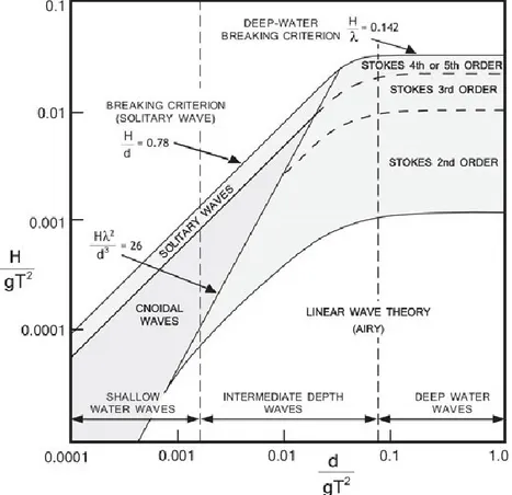
Figure 1. Applicability ranges of various wave theories (from Le Méhauté, 1969). d: mean water depth; H: wave height; T: wave period; g: gravitational acceleration. ... 8 Figure 2. A physical illustration of sinusoidal (a) and asymmetric (b) wave profiles. ... 10 Figure 3. Wave elevation signal: comparison of experiments with wave theories from

the work of Veic et al. (2016). ... 11 Figure 4. Breaking wave in deep ocean. Left panel: spilling breaking wave. Right

panel: plunging breaking wave. From Banner and Peregrine (1993). ... 12 Figure 5. Meaning of the KC number: definition sketch. From Sumer and Fredsøe

(2006). ... 18 Figure 6. Regimes of flow around a smooth, circular cylinder in an oscillatory flow.

Re = 103. ... 19 Figure 7. Vortex shedding regimes around a smooth circular cylinder in an oscillator

flow. NL is the number of oscillations in the lift force per flow cycle. From Sumer and Fredsøe (2006). ... 21 Figure 8. Wave force induced on a slender vertical cylinder: sketch for Morison’s

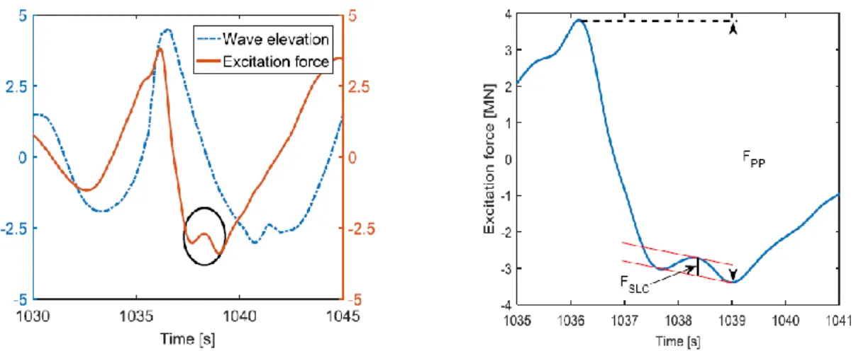
formulation. From Matteotti (1995). ... 22 Figure 9. Sketch for the breaking wave impact force. ... 24 Figure 10. Occurrence of the secondary load cycle, visible on the excitation force

(left panel). Estimation of FSLC parameter (right panel). From

Suja-Thauvin et al.(2017)... 28 Figure 11. Cross-correlation. Top panel: Example of the formation of the correlation

plane by direct cross-correlation: here a 4×4 pixel template is correlated with a larger 8×8 pixel sample to produce a 5×5 pixel correlation plane.

Bottom panel: Composition of peaks in the cross-correlation function.

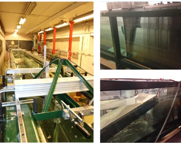
From Raffel et al. (1998). ... 32 Figure 12. The medium-size wave flume of the Hydrodynamics Laboratory (left

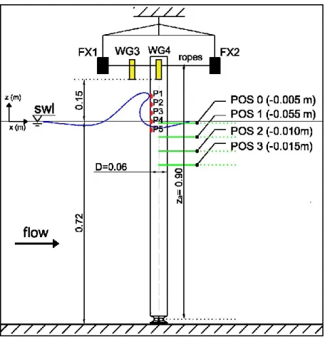
panel). Details of the wavemaker (top right panel) and of the absorbed beach (bottom right panel). ... 44 Figure 13. Global sketch of the experimental setups. The cylinder reports all

instruments in use: wave gauges close to the cylinder (WG3, WG4, in yellow) and force measurements system (FX1, FX2, in black) common to

(14)

both configurations; pressure transducers (P1-P5, red dots) relative to Setup1 and horizontal sheets (POS0-POS4, green lines) relative to

Setup2. Dimensions are expressed in m. ... 46

Figure 14. Acoustic wave gauges system for measurements of the water level. Left panel: in-line arrangement of acoustic wave gauge. Right panel: acquisition controller box. ... 47

Figure 15. Force measurement system arrangement. Left panel: general view. Right panel: detail of load cell. ... 48

Figure 16. Miniaturized pressure transducer. ... 49

Figure 17. Light sources: LED line (left panel) and laser (right panel). ... 51

Figure 18. CCD cameras. Left panel: Teledyne DALSA. Right panel: Photron FASTCAM SA5. ... 52

Figure 19. Seeding particles. ... 52

Figure 20. Timing diagram of the synchronization system related to the Setup 2. ... 54

Figure 21. Setup1. Configuration of pressure transducers, namely P1 to P5, from top to bottom. Left panel: cylinder with pressure transducers at the frontline, i.e. the rotation of the cylinder is equal to 0°. Right panel: counterclockwise rotation of 15° of the cylinder with pressure transducers. ... 56

Figure 22. View of the final configuration of Setup1, right after the seeding with particles. ... 57

Figure 23. Sketch of the PIV arrangement for Setup2. ... 58

Figure 24. View of the final configuration of Setup2, during a PIV acquisition. ... 59

Figure 25. Example of curve fitting on wave 3.1. ... 65

Figure 26. Example of filtering of a force signal: wave 1.1 (top panel) and 4.1 (bottom panel). ... 66

Figure 27 Example of instantaneous velocity field from PIV analysis: case 1.1 (left panel) and case 3.1 (right panel), at different times subsequent to the wave passage, with incident flow from bottom to top. ... 68

Figure 28. Vortex evolution for case 1.1. Top panel: Time history of the wave elevation. Bottom panel: Vorticity maps at times (A-D) and at horizontal planes (POS1-POS3). Incident flow from bottom to top. ... 72

Figure 29. Vortex evolution for case 3.1. Top panel: Time history of the wave elevation. Bottom panel: Vorticity maps at times (A-D) and at horizontal planes (POS1-POS3). Incident flow from bottom to top. ... 73

Figure 30. Vortex evolution for case 3.3. Top panel: Time history of the wave elevation. Bottom panel: Vorticity maps at times (A-D) and at horizontal planes (POS1-POS3). Incident flow from bottom to top. ... 74 Figure 31. Vortex evolution for case 4.1. Top panel: Time history of the wave

(15)

Figure 32. SLC dynamics for case 1.1. Top panel: Time histories of wave elevation (in blue) and wave-exciting moment (in red). Bottom panel: Evolution of the vorticity at times (A’-D’) significant for the SLC, and at horizontal planes (POS1-POS3). Incident flow from bottom to top. ... 77 Figure 33. SLC dynamics for case 2.1. Top panel: Time histories of wave elevation

(in blue) and wave-exciting moment (in red). Bottom panel: Evolution of the vorticity at times (A’-D’) significant for the SLC, and at horizontal planes (POS1-POS3). Incident flow from bottom to top. ... 79 Figure 34. SLC dynamics for case 3.1. Top panel: Time histories of wave elevation

(in blue) and wave-exciting moment (in red). Bottom panel: Evolution of the vorticity at times (A’-D’) significant for the SLC, and at horizontal planes (POS1-POS3). Incident flow from bottom to top. ... 80 Figure 35.. SLC dynamics for case 4.1. Top panel: Time histories of wave elevation

(in blue) and wave-exciting moment (in red). Bottom panel: Evolution of the vorticity at times (A’-D’) significant for the SLC, and at horizontal planes (POS1-POS3). Incident flow from bottom to top. ... 81 Figure 36. Vortex-induced force evaluation for case 1.1. Top panel: Time histories of

measurement wave-induced force on the cylinder (in black) and calculated transversal (in red) and inline (in blue) drag force components induced by vorticity, at the elevations corresponding to horizontal planes (POS1-POS3). Bottom panel: evolution of the vorticity at significant times (A”-E”), and at horizontal planes (POS1-POS3). Incident flow from bottom to top. ... 86 Figure 37. Vortex-induced force evaluation for case 4.1. Top panel: Time histories of

measurement wave-induced force on the cylinder (in black) and calculated transversal (in red) and inline (in blue) drag force components induced by vorticity, at the elevations corresponding to horizontal planes (POS1-POS3). Bottom panel: evolution of the vorticity at significant times (A”-E”), and at horizontal planes (POS1-POS3). Incident flow from bottom to top. ... 91

(16)

Figure 40 Vortex-induced force evaluation for case 3.3. Top panel: Time histories of measurement wave-induced force on the cylinder (in black) and calculated transversal (in red) and inline (in blue) drag force components induced by vorticity, at the elevations corresponding to horizontal planes (POS1-POS3). Bottom panel: evolution of the vorticity at significant times (A”-E”), and at horizontal planes (POS1-POS3). Incident flow from bottom to top. ... 92 Figure 41. Extreme response events identification. Experimental data (red markers)

and data by Riise et. al, 2018 (black dots). Open square: vorticity generation occurrence with no SLC (case 3.1). Filled square: vorticity generation and SLC (cases 1.1, 1.2, 3.1, 4.1). Open triangle: no vorticity, presence of SLC (cases 2.1, 2.3). Dashed line: KC=0.5. Continuous line:

(17)

List of Tables

Table 1. Position of the investigated horizontal light sheets on the backside of the cylinder. ... 59 Table 2. Parameters of the tested waves: ηc surface elevation at the crest measured

by WG4, Ttt trough-to-trough period, Tf zero up-crossing period of the

force history, Tav=(Ttt+Tf )/2 average period, L wave length, k wave

number, kηc wave slope, kR dimensionless wave number with respect to

the cylinder radius, Re Reynolds number, KC Keulegan-Carpenter number and Fr Froude number. ... 62 Table 3. Reorganized parameters of the tested waves in light of results available: ηc

surface elevation at the crest measured by WG4, Ttt trough-to-trough

period, Tf zero up-crossing period of the force history, Tav*

dimensionless average period, L wave length, k wave number, kηc wave

slope, kR dimensionless wave number (with respect to the cylinder radius), Re Reynolds number, KC Keulegan-Carpenter number and Fr Froude number. VG means Vortex Generation, while SLC secondary load cycle, whose presence is indicated by ‘Y’(yes) or ‘N’ (no). ... 98

(18)

Chapter 1 INTRODUCTION

In the last decades, the worldwide increasing demand for energy, especially from the renewable forms, such as wind power plants, led the offshore industry to move its activities towards deeper waters. Although the aim is to enhance the energy production, an increase in installation and maintenance costs must be faced because structures are more often exposed to high dynamic loads caused by the harsh environment, thus they are more prone to be damaged (for example by fatigue, vibrations and resonance). Starting from the observation of episodes of damages involving offshore structures, especially on platforms and wind turbines mainly constituted by cylindrical sub-structures, it has been revealed (Jefferys and Rainey, 1994; Faltinsen et al., 1995; Chaplin et al., 1997) that even the impact of steep waves, both breaking and near-breaking waves, may induce destructive effects such as ringing, a high frequency transient resonant response of the structure that may arise even if the wave period is far from the eigenperiod of the structure (Stansberg et al., 1995; Marthinsen et al., 1996; Welch et al., 1999). Notwithstanding the many efforts made by the research community on the comprehension of the phenomenon, its causes of occurrence and effects are still not fully understood.

Thesis objective

1.1

The present thesis aims to improve the knowledge on the dynamic processes arising around a vertical slender cylinder hit by a steep wave, breaking and non-breaking, in deep waters. Specific focus is on the secondary load cycle, a second load peak arising after the main peak in force signal, whose connection with the ringing phenomenon is likely.

(19)

Findings on the generation mechanisms of the secondary load cycle are still insufficient, thus an experimental campaign was conducted aimed at collecting useful data and information on this phenomenon.

In light of the complexity of the topic, which involves several nonlinear processes, such as the breaking and the impulsive nature of the wave-induced load on the structure, a broad investigation is needed. The laboratory experiments have been designed mainly focusing on the investigation of flow separation and vortex formation on the downstream side of the cylinder, in conjunction both with the identification of the specific features of the measured force signal, e.g. the second load cycle, and with the incoming wave characteristics.

The broad overview of the results coming from the experiments, that covered all the above-mentioned aspects, may constitute the ground on which to build an interpretation of the conditions that give rise to the higher-order response of vertical cylinders in deep waters when they are exposed to steep waves.

The present research has been undertaken in an effort to improve the understanding the ringing phenomenon in view of the applications typical of the oil and gas industries, renewable energy industries and the scientific community. It is widely recognized that ringing-induced excitation threatens the safety of offshore structures, and, therefore, arise the need to take it into consideration within standards codes as an important issue during the design process.

Background

1.2

Steep near-breaking and breaking waves, likely occurring in deep waters, make structures suffered to large high-frequency loads, in the same extent of more extreme wave events. Furthermore, the nonlinear inertia loading transferred by steep waves contributes to the high-frequency ringing response build-up in structures, together with the nonlinearity of the wave motion and of the dynamic response of the structure itself (Tromans et al., 2006). Ringing generates very high stress level with a burst of only a few higher harmonic oscillations (Chaplin et al., 1997) and imposes a serious potential danger to the structures.

(20)

Field observations revealed that cylindrical monopiles, which are by far the most popular support structures for gravity-based platforms (GBS) and wind turbine substructures, being also used in tension-leg platforms (TLP), may be affected by ringing. The first observations of the ringing responses date back to the mid-1990s and were obtained at the Hutton and Heidrun oil production platforms and at the deep water concrete towers of Draugen and Troll platforms in the Norwegian Sea fields (Natvig and Teigen, 1993). Evidence of these tests was discussed also in Jefferys and Rainey (1994), reporting examples of the ringing-type responses from the Heidrun model tests. Again, the occurrence of ringing was also observed at the Norwegian oil production Gullfaks C during operation in storm conditions (Langen et al., 1998).

These experiences motivated the significant amount of research that followed over the years. On the theoretical side, it is worth recalling the relevant efforts on the estimation of higher-order harmonic force on cylinders. An analytical solution accounting up to the third-harmonic of the wave forcing by regular waves in deep water was derived by Faltinsen et al. (1995a). This is known as the FNV method, and has been recently generalized to finite water depths by Kristiansen and Faltinsen (2017), whereas third-harmonic forces theories for irregular waves were presented by Newman (1996), Krokstad et al. (1998) and Johannessen (2011).

Recently, the strong worldwide incentive towards renewable energy, which has driven the development of wind farms, which are planned to expand more and more, renewed the interest in the investigation of higher-harmonic wave loads and in the prediction of the associated ringing phenomenon. The concern arise from the fact that, the trend in increasing the size of the offshore wind turbines together with the limited blade tip velocity, led to a decrease of the natural frequencies of the support structures, thus making these structures more prone to ringing responses (Suja-Thauvin et al., 2014).

The problem of predicting the ringing response, in terms of identification of hydrodynamic processes at the base of higher-harmonic load phenomena and ringing occurrence, have stimulated many experimental and numerical studies over the years. Particular focus has been on the investigation of the flow characteristics at and forces on the cylinders exposed to steep waves.

(21)

The early experiment in infinite water depths was conducted by Grue et al. (1993) on restrained vertical cylinder. A higher harmonic oscillation was first identified in the recorded force measurements for certain values of wave height. This phenomenon, called

secondary load cycle, was also reported by Chaplin et al. (1997) and Chaplin and Rainey

(2003) as due to focusing waves and by Grue and Huseby (2002) as evolving during the transient of a regular wave train; the same phenomenon has been observed by Stansberg et al. (1995) as forced by irregular waves.

The secondary load cycle looks like an additional force peak that occurs shortly prior to the time of minimum loading, at about one quarter wave period after the force main peak, and lasts for about 15% of the wave period (Grue et al., 1993). Grue and Huseby (2002) investigated the secondary load cycle for both a small and a moderate scale cylinder, i.e. for cylinder of radius 3cm and 6cm respectively. They found that the occurrence of the secondary load cycle depends on the wave steepness, in agreement with Chaplin et al. (1997). In particular, in small-scale experiments, the secondary load cycle was observed for waves of slope kηc>0.3 in the range of kD<0.66, where k is the wavenumber, ηc the

wave elevation at crest and D the diameter of the cylinder; whereas for moderate-scale, the phenomenon was observed for smaller wave slopes. Furthermore, Grue and Huseby (2002) suggested the Froude number Fr (Fr_c gD where ω is the wave frequency) as a governing parameter for the secondary load cycle, reporting the occurrence of such small-scale load for Fr>0.35. These trends in the occurrence of the phenomenon have been confirmed also by the most recent experiences (Li et al., 2014; Suja-Thauvin et al., 2017; Fan et al., 2018; Riise et al., 2018b, 2018a; Liu et al., 2019 ).

The secondary load cycle has been regarded to largely contribute to the higher-harmonic component of the total force exerted by incident steep waves on the cylinder (Grue et al., 1993) and this aspect has been put in relation with the ringing motion of vertical cylinders (Chaplin et al., 1997; Stansberg, 1997; Grue and Huseby, 2002) . However, a comprehensive knowledge of the ringing generations mechanisms is still lacking and the origin of the secondary load cycle, and its possible relation with the ringing occurrence, are still under discussion.

Grue and Huseby (2002) documented that pronounced ringing occurs for the same wave parameters as a secondary load cycle in the wave force. Besides, they attributed the

(22)

appearance of the secondary load cycle to a suction force acting at about one cylinder radius below the still-water level and describe the phenomenon as a resonance between a local induced flow and the cylinder. The conjecture that the secondary load may be a cause of ringing response has been supported also by the works of Chaplin et al. (1997),.Suja-Thauvin and Krokstad (2016) and Riise et al. (2018b).

Differently, Rainey (2007) ascribed the origin of the secondary load cycle to a kind of wave run-up on the downstream side of the cylinder, in agreement also with evidences by Krokstad and Solaas (2000), thus attributing no direct connection with the nonlinear behaviour of the ringing force. Other experimental tests, concerning steep and breaking irregular waves on cylinders (Bachynski et al., 2017; Suja-Thauvin et al., 2017) reported both the secondary load cycle and ringing response, but without finding a correlation between the characteristics of the two phenomena. In fact, some ringing events occurred with no presence of secondary load cycle, suggesting that the secondary load cycle does not necessary induce ringing response.

More recently, computational fluid dynamics models have been used to study the higher harmonic wave loads in periodic waves. Paulsen et al., 2014 discussed the physics of the secondary load cycle, recognizing it as "[...] an indicator of strong non-linear flow more

than a contributor to the resonant forcing". In addition, the observation of a rather strong

vortex downstream the cylinder owing to the return flow that has been seen in conjuction with the secondary load cycle, suggested it could contribute to the origin of the secondary load cycle. Lately, a similar CFD-calculation of such large vortex formation was presented as part of the theoretical and experimental study by Kristiansen and Faltinsen (2017), also in periodic waves. Moreover, with the aim to include turbulence effects, the numerical study by Liu et al. (2019) in breaking waves, pointed out a process of water up-rushing on the back of the cylinder just after the wave front had passed the cylinder, at which the secondary load cycle begins to occur and develops up to vanishing.

Those latter studies have opened a new direction of investigation of the topic focused on the role of flow separation and vortex formation which is still poorly explored.

(23)

Outlines of the thesis

1.3

This thesis starts with a short overview of the main theoretical fundamentals at the basis of the investigated phenomena. Wave theories regarding solitary and breaking waves in deep water are reported in Chapter 2, together with aspects relative to the hydrodynamics induced by these waves on vertical slender cylinders. Focus on higher-harmonic wave load is given and an analytical description of waves is provided therein.

Chapter 3 includes a theoretical description and practical information of the measuring methods used in the thesis. Several different aspects are covered. First, a short introduction to Particle Image Velocimetry (PIV) and the analysis of images are given. Secondly, a description of the wave focusing generation technique is provided. Finally, a discussion on vortex identification criteria in literature is developed.

A practical full description of the experiments, measuring tools and experimental techniques is illustrated in Chapter 4. Experimental setups are described in detail, pointing out the difficulties in their realization. The laboratory instruments needed for the work are described. Information about the wave input and the wave characterization is also given. The main PIV results, in terms of vorticity and velocity fields, are discussed in conjunction to both force and surface elevation signals in Chapter 5. The secondary load cycle occurrence is discussed. A brief summary of the results and suggestions for further improvements of the work can be found in Chapter 6.

(24)

Chapter 2 THEORETICAL FUNDAMENTALS

Deep-water wave theory

2.1

The great variety of water waves, e.g. from storm waves generated by wind, to seiches in harbour basins, up to tsunami waves generated by earthquakes, to name but a few, makes it evident that a general analytical solution of wave motion does not exist. Indeed, a large amount of physical aspects are involved in the generation and characterization of wave motion.

Numerous water wave theories have been thus developed providing approximate solutions for the study of wave motion which are applicable to different environments dependent on the specific environmental parameters, e.g. water depth, wave height and wave period. Because of the simplifying assumptions to be introduced in the attempt for giving solutions, a water wave theory is valid within its own established limits of applicability. One of the main challenges for engineers is the adoption of the most appropriate mathematical approach valid for the description of the problem under study.

Figure 1 illustrates qualitatively the range of validity of the main wave theories in literature. The regions are described in terms of H/T2 and d/T2, i.e. of wave height H and water depth d in relation to wave period T. Water depth is used to distinguish between shallow-water waves for d/L< 0.05 and deep-water waves for d/L> 0.5 (where L is the wavelength), while in between (see the vertical dashed lines in the graph) are intermediate depth waves. Waves in shallow water are significantly affected during their propagation to

(25)

shore by seabed level changes, while deep water waves are not affected by the seabed topography.

Figure 1. Applicability ranges of various wave theories (from Le Méhauté, 1969). d: mean water depth; H: wave height; T: wave period; g: gravitational acceleration.

The graph is limited by a breaking criteria which implies that there is a maximum value for the wave steepness, which is function of the relative depth. A number of equivalent definitions have been provided for breaking criteria. Breaking occurs when: a) the particle velocity at the crest becomes larger than the wave velocity, b) the pressure at the surface is incompatible with the atmospheric pressure, c) the particle acceleration at the crest tends to separate the particles from the bulk of water surface, d) the free surface becomes vertical. Accordingly, the following theoretical limits were reported in the graph:

In deep water (Mitchell limit)

𝐻

𝐿 < 0.142 (2.1)

In intermediate water depth (Miche formula) 𝐻 𝐿 < 0.14tanh( 2𝜋𝑑 𝐿 ) (2.2)

(26)

In case of solitary waves 𝐻

𝑑 = 0.78

(2.3)

The analyses that follow focus on deep-water wave theories, which are limited to a flat bottom and a constant uniform water depth. In the framework of the theories most commonly used in the design of offshore structures, they are: (1) linear Airy wave theory, (2) Stokes higher-order theory and (3) stream function theory. A brief discussion on their limits and regions of applicability is developed, following Chakrabarti (1987).

At the basis of all water wave theories there are the assumptions of two dimensional periodic and uniform waves, of horizontal ocean floor giving constant depth d from the still water level (swl) and of progressive waves in the horizontal direction. The main challenge for any wave theory is to determine the unknown boundary condition of the free surface, starting from the solution of the velocity potential, Φ or, equivalently, of the stream function, Ψ. Airy and Stokes formulations are based on the potential function and are developed around the wave height as a perturbation parameter that is limited to a given order of the wave theory. Differently, the stream function is expressed in a general order and a numerical solution is sought from the formulation.

The small amplitude wave theory is the simplest and most used of all theories. It is based on the assumption that the wave height is small compared to both wave length and water depth. With this assumption, the free surface boundary conditions can be linearized by neglecting the wave height terms beyond the first order. The solution of Φ takes the form of a power series in terms of a non-dimensional perturbation parameter ε, defined as the wave slope (wave height/wave length) as  ak, in which k is the wave number, defined as k 2 L and a is the amplitude, here equal to H/2. The linear theory gives symmetric profiles about the swl and it is upper limited by the wave height at which waves becomes unstable and break. In deep water the limiting wave steepness is represented by the Mitchell limit reported by Equation 2.1.

Around this steepness limit, the loss in symmetry of the wave surface is relevant. Asymmetry consists in the wave crest becoming more and more narrow and steep, whereas the wave trough becomes long and flat (Figure 2). Nonlinearity of wave manifests itself in

(27)

an increased steepness of the wave, and so the sinusoidal wave theory by Airy breaks down. Higher order perturbation solutions must, therefore, be adopted.

Stokes employed the perturbation technique and expanded the solution to higher orders, taking into account the nonlinear part of the solution. This formulation is taken to be valid for H d

 

kd 2, for (kd)<1 and H/L<<1 which constitute severe restrictions on the wave heights in shallow water, thus the Stokes theory is not generally applicable to shallow-water waves.

Figure 2. A physical illustration of sinusoidal (a) and asymmetric (b) wave profiles. From Le Méhauté (1969).

Perturbative terms of increasing order are included in the velocity potential expression as the higher order considered. The mathematics is clearly more cumbersome and complexity increases with the increase in accuracy, but Stokes formulation up to the fifth-order and coefficients formulations are provided in literature (Skjelbreia and Hendrickson, 1960). Not reported in the graph, but well known in literature, is the stream function theory developed by Dean (1965). It is a nonlinear wave theory, related to that of Stokes, but based on a stream function representation of the flow. A more detailed description of this theory is beyond the scope of this discussion, but it would point out the advantage that no restriction is imposed to the wave form. The wave can change form as it propagates due to the interaction of components at various phase speeds and relative motion. In general, the stream function theory may be appropriate and consistent over most of the wave parameter domain of Figure 1 except at very low ends of the values.

In conclusion, in deep water (d/L> 0.5 or d/T2> 1), the Stokes nonlinear theory is more appropriate to describe waves fitting the near-breaking conditions with increasing accuracy for increasing order of expansion. However, the best fit for the kinematic condition is

(28)

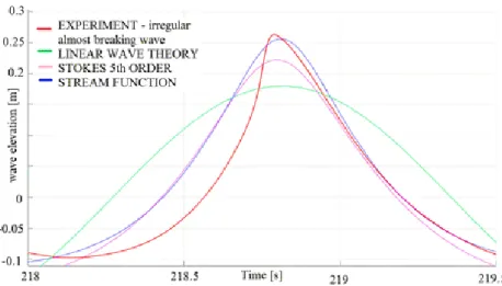
found for the stream function theory. Figure 3 is reported as example of the wave description provided by the above-mentioned wave theories, noting that steep waves in deep water need to be described by nonlinear wave theories.

Figure 3. Wave elevation signal: comparison of experiments with wave theories from the work of Veic et al. (2016).

Breaking waves in deep waters

2.1.1

Breaking waves play an important role in the exchange of mass, momentum, energy transfer between the atmosphere and the sea, which may have effects on climate as well as in turbulence generation and turbulence-wave interactions. Furthermore, knowledge of hydrodynamics of breaking waves has always been sought by the engineers community, interested in improving the design procedures of marine structures often subjected to impulsive and extreme wave loads transferred by breaking waves.

In nature, wave breaking can be observed in the open ocean as well as in regions near the coastline, but with completely different generating processes. Breaking waves are generally divided into two regimes: deep water breaking waves, where the water is sufficiently deep that the waves are not affected by the seabed topography, and shallow

water breaking waves, where the waves break due to effects induced by changes in water

depth.

(29)

and measurements in the field have shown that breaking waves are universally present over the ocean surface as well as in all environments where the deep-water condition is reached.

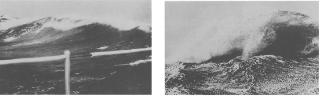
In this environment, two types of breaking waves were observed. Spilling (Figure 4, left panel) is the more typical breaking type in deep water. Spilling breaking waves are characterized by white-capping near the crest, due to entrained wave bubbles and drops created at the surface, gently spreading down the forward face of the wave. Secondly,

plunging breakers (Figure 4, right panel) can occur, where the forward face of the breaker

overturns violently into the slope of the preceding trough, causing splashes, eddies and large air entrainment. Even if the plunging breakers are more common on beaches, they may occur, with less frequency than spilling, also in deep water, usually during severe storms and represent the most dramatic event.

Figure 4. Breaking wave in deep ocean. Left panel: spilling breaking wave. Right panel: plunging breaking wave. From Banner and Peregrine (1993).

It is widely recognized that an individual wave breaking event starts when water particles near the wave crest develop a velocity in the wave propagation direction sufficiently large from them to fall down the front of the wave. If on one hand this phenomenon is evident during the propagation of a wave toward the shore, where the wave become steeper due to the effects of the variation of the seabed topography, on the other hand less intuitive are the mechanisms of generation of wave breaking in deep waters and the definition of the breaking criteria.

Direct observations in field and a large amount of investigation show that breaking in deep water may result from: i) the interaction of waves and currents, ii) direct forcing by wind

(30)

(Phillips, 1977), iii) intrinsic instabilities of the wave field (Melville, 1982), and iv) the constructive interference of a number of Fourier components. Melville and Rapp (1988) supported that the latest of such mechanisms may be the most important for waves near the peak of the spectrum, whereas the direct effect of wind forcing is likely to be of little significance near the peak of the spectrum, but may dominate at higher frequencies.

Especially in a random sea, where waves with different propagation directions interact, the superposition of wave components at different frequencies can occur. This may lead to the generation of a highly asymmetric non-steady wave, that can break if it reaches a certain breaking limit. The classical breaking criterion is represented by the geometric criterion that a wave at the point of breaking is a Stokes wave with a limiting crest angle of 120° and a maximum steepness (ak)max = π/7. Although, this is usually applicable, rarely a

geometric criterion for breaking is applied because definition of wave height and slope can be ambiguous (Melville and Rapp, 1988). For this reason, the research moved towards the definition of global breaking criteria, also investigating the kinematics ( Kjeldsen et al., 1980; Bonmarin and Ramamonjiarisoa, 1985; Longuet-Higgins, 1988) or energetics (Schultz et al., 1994) of wave breaking.

Furthermore, several instability mechanisms were observed that can provoke wave breaking in deep water. Tanaka (1983, 1985) demonstrated that periodic waves with wave steepness greater than 0.43 are unstable, a discovery that led Jillians (1989) to investigate more on the evolution of instability and its role on the onset of breaking, who found that the instability is concentrated near the crest. Another form of instability regarding wave trains was found by Benjamin and Feir (1967), this consisting in an infinitesimal long modulations of a wave train growing in amplitude until strongly modulated wave groups occur. Finally, three-dimensional instability was observed for steeper deep-water wave trains in which alternate crests grow at the expenses of those in between (Longuet-Higgins, 1978).

Kinematic formulations for steep waves: the Stokes theory

2.1.2

With the assumptions of fluid incompressible, inviscid and irrotational, the flow can be described by the potential function (or velocity potential), Φ. The velocity potential Φ and

(31)

the surface displacement η are determined from solving Laplace's equation (Equation 2.4) for the given boundary conditions.

The free surface kinematic condition of Equation 2.5 states that a particle lying on the free surface remains on the free surface over time. The free surface dynamic condition, based on the assumption that the atmospheric pressure outside the fluid is constant, is reported Equation 2.6 Finally, the no-slip condition at the seabed states that the velocity is zero at the horizontal seabed (Equation 2.7).

For uniform depth, the boundary value problem to be solved is conclusively written as:

∇2_{Φ = 0} for – h < z < η _(2.4) 𝜕𝜂 𝜕𝑡 + 𝜕Φ 𝜕𝑥 𝜕𝜂 𝜕𝑡 − 𝜕Φ 𝜕𝑥 = 0 at z=η (2.5) 𝜕Φ 𝜕𝑡 + 1 2(∇ 2_{Φ) + 𝑔𝑧 = 0} at z=η _(2.6) 𝜕Φ 𝜕𝑧 = 0 at z=-h (2.7)

where x represents the horizontal axis and z the vertical axis of a two dimensional Cartesian coordinate system with origin at the undisturbed free surface.

The linear Airy theory provides the simplest way to predict the wave kinematics, under the assumption of small wave amplitude a with respect to the wave length. For a regular wave a possible solution to the linear problem is:

𝜂 = 𝑎 cos(𝑘𝑥 − 𝜔𝑡 + 𝜑) (2.8)

𝜙 = 𝑎𝜔cosh 𝑘(𝑧 + ℎ)

𝑘 sinh 𝑘ℎ sin(𝑘𝑥 − 𝜔𝑡 + 𝜑) (2.9)

where 2 T is the angular frequency, k and ω are related through the linear dispersion relation

(32)

ω2 = 𝑔𝑘 tanh 𝑘ℎ (2.10) and φ is a phase displacement, which may be set equal to zero with a suitable choice of the time/space origin.

Irregular waves may be composed by superposing plane wave components with different amplitudes and phases. By means of the linear Airy theory, the surface displacement and the potential function may appear as:

𝜂 =1 2∑(𝑎𝑗𝑒 𝑖(𝑘𝑗𝑥−𝜔𝑗𝑡)_{+ 𝑐. 𝑐)} 𝑗 (2.11) 𝜙 = −1 2∑ (𝑖𝑎𝑗𝜔𝑗 cosh 𝑘_𝑗(𝑧 + ℎ) 𝑘_𝑗sinh 𝑘_𝑗ℎ 𝑒 𝑖(𝑘𝑗𝑥−𝜔𝑗𝑡)_{+ 𝑐. 𝑐)} 𝑗 _(2.12)

where aj is a complex amplitude containing both the modulus of the amplitude |aj| and the

phase displacement φj = arg aj.

For the solution of the nonlinear boundary value problem, Stokes introduced harmonic power series in terms of a parameter containing the amplitude. In Stokes' original theory the parameter ε=ak was used to expand the series. Looking at the surface displacement the most noticeable higher order effect is the second order contribution that makes both the crest and trough higher. Skjelbreia and Hendrickson (1960) developed a fifth-order method to calculate both the surface displacement and the kinematics with ε=ak as the expansion parameter. Later, Fenton (1985) showed this method to be wrong at the fifth order and introduced the wave steepness ε=kH/2, where H is the wave height from crest to trough, as the expansion parameter.

Fenton's method for steady propagating waves at finite depth is:

𝜙 = (𝑐 − ū)𝑥 + 𝐶0√𝑔/𝑘3∑ 𝜖𝑖∑ 𝐴𝑖𝑗cosh 𝑗𝑘(𝑧 + ℎ) sin 𝑗𝑘(𝑥 − 𝑐𝑡) + 𝑂(𝜖6) 𝑖 𝑖=1 5 𝑖=1 (2.13) ū√𝑘/𝑔 = 𝐶₀+ 𝜖2𝐶₂+𝜖4𝐶₄+ 𝑂(𝜖6) (2.14)

(33)

𝑘𝜂 = 𝑘ℎ + 𝜖 cos 𝑘 (𝑥 − 𝑐𝑡) + 𝜖2_𝐵 22cos2 𝑘 (𝑥 − 𝑐𝑡) + 𝜖3𝐵31(cos 𝑘 (𝑥 − 𝑐𝑡) − 𝑐𝑜𝑠3𝑘(𝑥 − 𝑐𝑡)) + 𝜖4(𝐵42cos2 𝑘 (𝑥 − 𝑐𝑡) + 𝐵44cos4 𝑘 (𝑥 − 𝑐𝑡)) + 𝜖5_(−(𝐵 53+ 𝐵55)cos 𝑘 (𝑥 − 𝑐𝑡)+𝐵53𝑐𝑜𝑠3𝑘(𝑥 − 𝑐𝑡)+) + 𝐵55𝑐𝑜𝑠5𝑘(𝑥 − 𝑐𝑡) + 𝑂(𝜖6) (2.15)

where c=L/T and H are known. For cases where L and T are known the theory can be directly applied. Otherwise, it is necessary to specify the current or the mass flux. The A, B and C coefficients and additional ways to find the wave length and the wave period can be found in Fenton’s work (Fenton, 1985).

Grue’s method (Grue et al., 2003) offers a simple way to predict the wave kinematics in deep waters. For deep water a possible solution to the boundary value problem (Equations 2.4-2.7), using Stokes original parameter ε for the expansion, is:

𝑘𝜙 √𝑔/𝑘= 𝜖𝑒 𝑘𝑦_{sin(𝑘𝑥 − 𝜔𝑡) + 𝑂(𝜖}4₎ (2.16) 𝑘𝜂 = (1 +1 8𝜖 2_{) 𝜖 cos(𝑘𝑥 − 𝜔𝑡) +}1 2𝜖 2_{cos 2(𝑘𝑥 − 𝜔𝑡) +}3 8𝜖 3_{cos 3(𝑘𝑥 −} 𝜔𝑡) + 𝑂(𝜖4) (2.17) 𝜔 𝑔𝑘 = 1 + 𝜖 2_{+ 𝑂(𝜖}3₎ (2.18)

and for a wave event the maximum surface displacement is denoted ηc and

𝑘𝜂_𝑐 = 𝜖 +1 2𝜖

2₊1

2𝜖

3 _{+ 𝑂(𝜖}4₎ _(2.19)

The parameter ε is found by solving the two equations for frequency dispersion (Equation 2.17) and wave steepness (Equation 2.18)(2.13). In ω=2π/T the time scale T is the local wave period from trough-to-trough for the wave event.

(34)

The horizontal velocity is given by:

𝑢 =𝜕𝜙

𝜕𝑥 = 𝜖√𝑔/𝑘𝑒

𝑘𝑦_{cos(𝑘𝑥 − 𝜔𝑡)} _(2.20)

At crest the horizontal velocity reaches its maximum ucrest g keky. When the velocity

is made dimensionless with the reference velocity, the exponential profile ky ref crest/u e

u 

is obtained.

The simplicity of Grue's method comes from the deep water condition, where kh>> 1. When kh >> 1 the coefficients of the second and third-order terms of the velocity potential converge to zero. Looking at the velocity potential the only correction from the first to the third order is in the dispersion relation, where the amplitude is included at third order. For finite depths the solution that satisfies the third-order boundary conditions becomes considerably more complex (Riise, 2009).

Flow around a cylinder in oscillatory flow

2.2

The hydrodynamic quantities describing the flow around a smooth, circular cylinder in steady currents depend on the Reynolds number. In the case where the cylinder is exposed to an oscillatory flow additional dynamics described by the so-called Keulegan-Carpenter number appear. The Keulegan-Carpenter number, KC, is defined by:

𝐾𝐶 = 𝑈𝑚𝑇𝑤

𝐷 (2.21)

in which Um is the maximum velocity and Tw is the period of the oscillatory flow. If the

flow is sinusoidal with velocity given by:

𝑈 = 𝑈𝑚sin(𝜔𝑡) (2.22)

then, the maximum velocity is

𝑈 = 𝑎𝜔 =2𝜋𝑎

(35)

where a is the amplitude of the motion. For the sinusoidal case the KC number is, therefore, identical to:

𝐾𝐶 =2𝜋𝑎

𝐷 (2.24)

The angular frequency of the motion that appears in Equation 2.22 relates to the frequency

fw as

𝜔 = 2𝜋𝑓_𝑤 =2𝜋

𝑇_𝑤 (2.25)

The physical meaning of the KC number can probably be best explained with reference to Equation 2.24. The numerator on the right-hand-side of the equation is proportional to the stroke of the motion, namely 2a, while the denominator, the diameter of the cylinder D, represents the width of the cylinder (Figure 5). Small KC numbers, thus, mean that the orbital motion of the water particles is small relative to the total width of the cylinder. Stating that, when KC is very small, separation behind the cylinder is expected to not occur.

Figure 5. Meaning of the KC number: definition sketch. From Sumer and Fredsøe (2006). Large KC numbers, on the other hand, mean that the water particles travel quite large distances relative to the total width of the cylinder, resulting in separation and probably vortex shedding. For very large KC numbers (KC), it may be expected that the flow

(36)

Flow regime and vortex formation

2.2.1

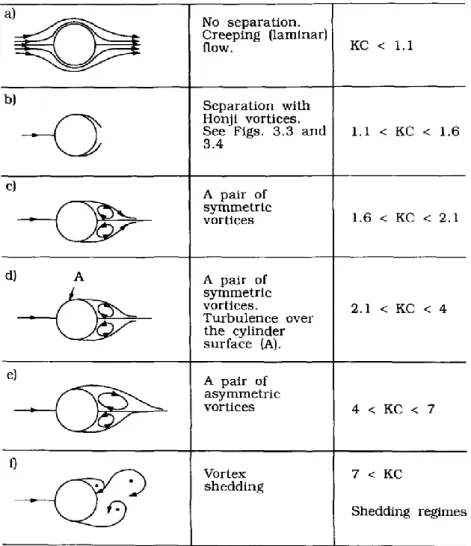
Figure 6 summarizes the most significant changes that occur in the flow around a vertical circular cylinder as the Keulegan-Carpenter number increases from zero. The images are related to the Reynolds number (Re = 103), which is defined as:

𝑅𝑒 = 𝑈𝑚𝐷

𝜈 (2.26)

and where ν is the kinematic viscosity of the fluid; for water ν=10-6m2/s.

Inspection at the table, from top to bottom, reveals that for very small values of KC no separation of the flow is present (Figure 6a), as expected.

Figure 6. Regimes of flow around a smooth, circular cylinder in an oscillatory flow. Re = 103_.

(37)

Separation first appears when KC is larger than 1.1 (Figure 6b). This occurs in the form of the so-called Honji instability. Reached this KC condition, the purely two-dimensional flow over the cylinder surface breaks into a three-dimensional flow pattern that exhibits repeatedly, in the cylinder’s length direction, pairs of rolls extending along the cylinder circumference. The pattern oscillates in time, appearing and disappearing with a cycle of period being half of the oscillation period. Visualization of these streaks by means of flow-visualization techniques, shows that fluid particles transported by the roll pairs may exhibit a periodic pattern of mushroom-shape vortices (Honji, 1981).

With a further increase of KC, separation occurs in the form of a pair of symmetric, ordinary, attached vortices (Figure 6c,d). This regime covers the KC range 1.6<KC<2.6 while the range 2.1<KC<4 is characterized by the appearance of turbulence over the cylinder (Sarpkaya, 1986), always for Re=103.

When KC increase even further, the symmetry between the two attached vortices breaks down (Figure 6e). The vortices remain attached to the cylinder, and no shedding occurs. The significance of this regime, prevailing over the range 4<KC<7, is that the lift force is no longer zero and this is caused by the asymmetry in the formation of the attached vortices.

For KC larger than 7, the vortex-shedding regime is established (Figure 6f). In this regime, the vortex shedding onset occurs during each half period of the oscillatory motion. Several such regimes can be distinguished, each of which has a different vortex flow pattern, observed for different ranges of the KC number, as discussed by Williamson (1985). The transverse-vortex-street regime is known to occur in the range 7<KC<13. A vortex street perpendicular to the flow direction is formed at the lower side of the cylinder. It consists in a pair of vortices, of opposite sign, that are alternatively shed from the side of the cylinder, each forced by the velocity field of the other (mutual induction). The position of the vortex street relative to the cylinder is connected to the direction of the lift force, which must be non-zero in this flow regime. With reference to the KC range 13<KC<15, the wake consists of a series of pairs convected away from the cylinder during each cycle at about 45° to the flow oscillation direction, and on one side of the cylinder only.

The Double-Pair regime occurs in the range 15<KC<24, in which the wake is the result of two vortices being shed at each half cycle. Two trails of vortex pairs move away from the cylinder in opposite directions and from opposite sides of the cylinder. For 24<KC<32,

(38)

the wake presents three vortices shed during a half cycle and three vortex pairs are comprised in a cycle. For higher KC regimes, the number of vortex pairs increases by one each time the KC regime is changed to a higher order, in the order of two more vortex sheddings each time a higher order is reached.

With reference to the effect of Re for large KC numbers (KC>3), the available data have been collected by Sumer and Fredsøe (2006) in a graph like that of Figure 7. No extensive data is provided in the literature. Nevertheless, Sumer and Fredsøe matched the extensive data by Sarpkaya (1976) covering a wide range of KC for lower Re regimes along with the data of Figure 7 to interpret what happens also for increasing Re numbers.

With reference to vortex-shedding, the figure shows that the curves begin to bend downward, as Re approaches the value 105. This means that in this region the normalized lift frequency NL, described as NL=fL/fw, where fL isthe fundamental lift frequency and fw is

the frequency of the oscillatory flow, increases with increasing Re. This is consistent with the corresponding result in steady currents, namely that the shedding frequency increases with increasing Re at 3.5×105 when the flow is switched from subcritical to supercritical through the critical (lower transition) flow regime.

Figure 7. Vortex shedding regimes around a smooth circular cylinder in an oscillator flow. NL is the number of oscillations in the lift force per flow cycle. From Sumer and Fredsøe (2006).

(39)

Wave loads on vertical slender cylinders

2.3

Wave forces on a vertical slender cylinder, i.e. a cylinder with diameter small compared to the water wave length, has proven to be well approximated by the Morison equation (Morison et al., 1950).

Figure 8. Wave force induced on a slender vertical cylinder: sketch for Morison’s formulation. From Matteotti (1995).

The Morison equation assumes the total in-line wave force to be composed by the inertia force (from potential theory and oscillating flow) and the drag forces (from real flows and constant currents) linearly added together (Equation 2.27).

𝐹(𝑡) = 𝐹𝑖𝑛𝑒𝑟𝑡𝑖𝑎(𝑡) + 𝐹𝑑𝑟𝑎𝑔(𝑡) = = ∫ 1 2 𝜂 −𝑑 𝜌𝐶_𝑀𝜋𝐷 2 4 𝑢̇(𝑧)𝑑𝑧 + ∫ 1 2 𝜂 −𝑑 𝜌𝐶_𝐷𝐷𝑢(𝑧)|𝑢(𝑧)|𝑑𝑧 (2.27) in which ρ is the water density and D, η and d were already defined in previous sections (see also Figure 8). CM and CD are two empirical coefficients, the inertia and the drag

coefficient, respectively.

The inertia force, representing the force opposed by the structure against the wave action, depends on the acceleration of the water particles 𝑢̇ = 𝑑𝑢/𝑑𝑡. Differently, the drag force, representing the drag action exerted by the wave on the cylinder due to the pressure differential created by the wake between the upstream and downstream sides of the cylinder, depends on the square of the water particle velocity, in the direction of wave

(40)

propagation. Therefore, the drag and the inertia force components are 90° out of phase with each other over time. It follows that, for small KC values, the inertia component of the in-line force is large compared with the drag component, thus in such cases the drag can be neglected. However, as the number of KC is increased, flow separation begins and the drag force becomes increasingly important.

The original form of the Morison equation is empirical. Over the years, its physical foundations have often been questioned, especially with regard to the dependency on the two empirical coefficient CM and CD and to the linear superposition of the two force

components, as well as to the validity of neglecting other forces, e.g. the wave run-up, the wave impact (slamming), the ringing, and so on.

Since the original Morison’s formulation was proposed under the assumption of small-amplitude waves, hence describing a quasi-static force action on a cylinder, such formulation would not be able to represent the load caused by an impulsive breaking event nor loads induced by random seas. While the Morison’s equation remains a proper engineering approximation, the wave condition for which this can be applied need to be investigated more in detail. Wave breaking, for example, may induce very high impact forces with extremely short duration on a slender structure, which is not taken into account in the original Morison’s formulation.

Wave breaking load

2.3.1

The impact forces generated by breaking waves can attain very large values. Works by Kjeldsen et al.(1986) and Basco and Niedzwecki (1989) showed that plunging wave forces on a pile can be 2-3 times larger than the ordinary forces with waves of comparable amplitudes. A similar multiplicative factor to Morison’s original formulation, established to be 2.5, is suggested by SPM 1984 in order to account for the impact force induced by a breaking wave. However, no information about the time history of this force is given. Under breaking wave attack, the description of the total breaking wave force must also include the additional impact force term Fimpact, (Wienke et al., 2000), which represents the

(41)

Therefore, Equation 2.27 changes in: 𝐹(𝑡) = 𝐹_{𝑖𝑛𝑒𝑟𝑡𝑖𝑎}(𝑡) + 𝐹𝑑𝑟𝑎𝑔(𝑡) + 𝐹𝑖𝑚𝑝𝑎𝑐𝑡(𝑡) = = ∫_−𝑑𝜂 1₂𝜌𝐶𝑀 𝜋𝐷2 4 𝑢̇(𝑧)𝑑𝑧 + ∫ 1 2 𝜂 −𝑑 𝜌𝐶𝐷𝐷𝑢(𝑧)|𝑢(𝑧)|𝑑𝑧 + 𝜌 𝐷 2 𝐶𝑏 2_𝐶 𝑠𝜆𝜂𝑏 (2.28)

where, relatively to Fimpact, Cb is the celerity at breaking, Cs is the slamming factor, λ is the

curling factor, which indicates how the wave crest is active in inducing a slamming force and it depends on the breaker type and the relative distance between breaking wave point and the structure location, and ηb is the maximum water surface elevation at the breaking

point (see also the sketch reported in Figure 9).

Figure 9. Sketch for the breaking wave impact force.

The analytical formulation for the impact force contribution is derived from calculations by Goda et al. (1966). It is assumed that the breaker front is vertical and moves with the wave celerity C, hitting the cylinder over the height of the impact area ληb. The maximum

line force on the cylinder is calculated by using Wagner or von Karman’s theory, respectively if considering or disregarding the flow besides the flat plate, with which cylinder is approximated (pile-up effect). Therefore, the slamming coefficient Cs is

(42)

approximatively twice the force and a half the duration of the impact with respect to what obtained by Goda et al. (1966). Similar results were obtained also by Sawaragi and Nochino (1984) and Chan et al. (1995).

Many studies over the years have been conducted aimed at improving the knowledge in the topic. As an example, we report, among them, the study by Wienke et al.(2001) on the curling factor determination relying on: i) the breaker type, ii) the classification of the breaking wave loads, iii) the relative distance between breaking point and position of the structure (Tanimoto et al., 1986; Wienke et al., 2000). We, finally, recall the large-scale model tests by Wienke and Oumeraci (2005) from which the three-dimensional force model used to estimate the maximum impact force on a slender cylinder has been recently developed.

Higher-order wave loads

2.3.2

The analysis of wave and corresponding structural responses are of great importance to ocean engineers in the design, and for the operational safety of offshore structures.

When a nonlinear wave, such as a steep wave, passes an offshore structure, the higher-order loads may in certain situations excite the structure as much as its natural frequencies. In an inner domain close to the body surface, in fact, the wave elevation is assumed to be significantly affected even by nonlinearities due to the presence of the structure causing wave diffraction and scattering. These nonlinear loads may induce undesired effects on the structures, such as vibrations.

Potential theory is usually used to investigate these effects, assuming viscous effects to be negligible.

The calculation of the first-order wave effects is regarded as straightforward and the linearized diffraction problem is well predicted by Morison equation, when only the inertia term is retained.

More interest is in the calculation of the higher-order wave effects. For tension leg platforms (TLPs) second-order wave loads have been found to induce resonant axial deflections of the tendons under moderate sea-state. This phenomenon is known as

(43)

springing and consists in steady-state oscillations, mainly caused by weakly nonlinear

forces at the second harmonic of the wave frequency. Springing loads have been calculated by Chen et al. (1991) and Eatock Taylor and Chau (1992).

Recently, TLPs and monopiles were found to be subjected to a transient resonance condition at their natural frequencies, substantially higher than the governing wave frequency (Faltinsen et al., 1995). This phenomenon involves harmonic wave load components higher than second order and it has become known as ringing. Ringing occurs as an axial deflection of the tendons of TLPs, and as a structural deflection in the bending mode for monopiles.

The cause of ringing is not still fully understood. It has been observed that ringing tends to occur when waves are steep and the wave amplitude is of the same order of the radius of the structure. Furthermore, the debate is still open on whether the nonlinear wave kinematics or the nonlinearities arising during wave-structure interaction is the most important factor.

Many different directions have been undertaken to calculate the third-order loads exactly, in order to investigate the ringing in more detail. One approach has been to extend the Morison equation, which gives good estimates for the first-order wave loads in long waves (Madsen, 1986; Rainey, 1989), which was used by Jefferys and Rainey (1994) to predict ringing. Another approach has been presented by Malenica and Molin (1995). They captured the complete third-order velocity potential for a fixed cylinder in finite depth based on the traditional Stokes perturbation method. Later, Faltinsen et al. (1995) presented the FNV theory, based on the long-wave approximation, which has been recently generalized to finite water depth (Kristiansen and Faltinsen, 2017).

The causes of the large higher-order loads have also been investigated experimentally and numerically. On the experimental side, Grue and Huseby (2002) documented that pronounced ringing occurs for the same wave parameters of a secondary load cycle in the wave force signal. This work drove many other experimental studies over the year, aimed at confirming or denying the connection between ringing and secondary load cycle occurrences.

On the numerical side, the more recent work by Paulsen et al., 2014a adds more information on the secondary load origin, but no connection with the ringing has been

(44)

found. Again, Kristiansen and Faltinsen (2017) states that the load associated with the run-up, generated by vortical structures arising by flow separation, and the subsequent propagation of steep local waves are the cause of large higher-order loads.

Secondary load cycle

2.3.2.1

Beyond its likely association with ringing, the secondary load cycle is a strongly nonlinear phenomenon regarding the wave load on the vertical cylinder. Indeed, Paulsen et al., 2014 found, in their experience, the secondary load cycle to belong to a frequency range above the sixth-harmonic wave frequency.

The secondary load cycle appears as a rapid and high-frequency increase of the excitation force and, occurs after the main peak in the load time-series, at the time of minimum loading (Figure 10, left panel).

The phenomenon was firstly described by Grue et al. (1993) from their experiments. The secondary load can be identified by some own characteristics. For example, it typically occurs about one quarter wave period after the main peak of the excitation force (Grue and Huseby, 2002) and it lasts for about 15% of the wave period (Grue et al., 1993).

Grue and Huseby (2002) further suggested some parameters that are currently used both as tools for the identification of secondary load occurrence and for the investigation of the causes and effects connecting on it. Among them, there are some wave parameters; in particular KC, measuring the flow separation effects, the Froude number Fr, measuring the role of surface gravity waves, the dimensionless wave slope kηc and the wave number kR.

The secondary load cycle has been observed for KC>4-5, Fr~0.35-0.4, kηc>0.3 and kR>0.1. The intensity of the secondary load cycle can be estimated by the SLC ratio,

defined as SLC=FSLC/FPP, i.e. its magnitude over the peak-to-peak force (Figure 10, right

(45)

Figure 10. Occurrence of the secondary load cycle, visible on the excitation force (left panel). Estimation of