2020-06-29T09:55:46Z
Acceptance in OA@INAF
ALMA Spectroscopic Survey in the Hubble Ultra Deep Field: CO Luminosity
Functions and the Evolution of the Cosmic Density of Molecular Gas
Title
DECARLI, ROBERTO; Walter, Fabian; Aravena, Manuel; Carilli, Chris; Bouwens,
Rychard; et al.
Authors
10.3847/1538-4357/833/1/69
DOI
http://hdl.handle.net/20.500.12386/26260
Handle
THE ASTROPHYSICAL JOURNAL
Journal
833
ALMA SPECTROSCOPIC SURVEY IN THE HUBBLE ULTRA DEEP FIELD: CO LUMINOSITY FUNCTIONS
AND THE EVOLUTION OF THE COSMIC DENSITY OF MOLECULAR GAS
Roberto Decarli1, Fabian Walter1,2,3, Manuel Aravena4, Chris Carilli3,5, Rychard Bouwens6, Elisabete da Cunha7,8, Emanuele Daddi9, R. J. Ivison10,11, Gergö Popping10, Dominik Riechers12, Ian R. Smail13, Mark Swinbank14, Axel Weiss15, Timo Anguita15,16, Roberto J. Assef4, Franz E. Bauer16,17,18, Eric F. Bell19, Frank Bertoldi20,
Scott Chapman21, Luis Colina22, Paulo C. Cortes23,24, Pierre Cox23, Mark Dickinson25, David Elbaz9, Jorge GÓnzalez-LÓpez17, Edo Ibar26, Leopoldo Infante17, Jacqueline Hodge6, Alex Karim20, Olivier Le Fevre27,
Benjamin Magnelli20, Roberto Neri28, Pascal Oesch29, Kazuaki Ota5,30, Hans-Walter Rix1, Mark Sargent31, Kartik Sheth32, Arjen van der Wel1, Paul van der Werf6, and Jeff Wagg33
1
Max-Planck Institut für Astronomie, Königstuhl 17, D-69117, Heidelberg, Germany;[email protected] 2
Astronomy Department, California Institute of Technology, MC105-24, Pasadena, CA 91125, USA
3
National Radio Astronomy Observatory, Pete V. Domenici Array Science Center, P.O. Box O, Socorro, NM 87801, USA
4
Núcleo de Astronomía, Facultad de Ingeniería, Universidad Diego Portales, Av. Ejército 441, Santiago, Chile
5
Cavendish Laboratory, University of Cambridge, 19 J. J. Thomson Avenue, Cambridge CB3 0HE, UK
6
Leiden Observatory, Leiden University, P.O. Box 9513, NL2300 RA Leiden, The Netherlands
7
Centre for Astrophysics and Supercomputing, Swinburne University of Technology, Hawthorn, Victoria 3122, Australia
8
Research School of Astronomy and Astrophysics, Australian National University, Canberra, ACT 2611, Australia
9
Laboratoire AIM, CEA/DSM-CNRS-Université Paris Diderot, Irfu/Service d’Astrophysique, CEA Saclay, Orme des Merisiers, F-91191 Gif-sur-Yvette cedex, France
10
European Southern Observatory, Karl-Schwarzschild-Strasse 2, D-85748, Garching, Germany
11
Institute for Astronomy, University of Edinburgh, Royal Observatory, Blackford Hill, Edinburgh EH9 3HJ, UK
12
Cornell University, 220 Space Sciences Building, Ithaca, NY 14853, USA
13
6 Centre for Extragalactic Astronomy, Department of Physics, Durham University, South Road, Durham DH1 3LE, UK
14
Max-Planck-Institut für Radioastronomie, Auf dem Hügel 69, D-053121 Bonn, Germany
15
Departamento de Ciencias Físicas, Universidad Andres Bello, Fernandez Concha 700, Las Condes, Santiago, Chile
16
Millennium Institute of Astrophysics(MAS), Nuncio Monseñor Sótero Sanz 100, Providencia, Santiago, Chile
17
Instituto de Astrofísica, Facultad de Física, Pontificia Universidad Católica de Chile, Av. Vicuña Mackenna 4860, 782-0436 Macul, Santiago, Chile
18
Space Science Institute, 4750 Walnut Street, Suite 205, Boulder, CO 80301, USA
19
Department of Astronomy, University of Michigan, 1085 South University Ave., Ann Arbor, MI 48109, USA
20
Argelander Institute for Astronomy, University of Bonn, Auf dem Hügel 71, D-53121 Bonn, Germany
21
Dalhousie University, Halifax, Nova Scotia, Canada
22
ASTRO-UAM, UAM, Unidad Asociada CSIC, Spain
23Joint ALMA Observatory—ESO, Av. Alonso de Córdova, 3104, Santiago, Chile 24
National Radio Astronomy Observatory, 520 Edgemont Rd, Charlottesville, VA 22903, USA
25
Steward Observatory, University of Arizona, 933 N. Cherry St., Tucson, AZ 85721, USA
26
Instituto de Física y Astronomía, Universidad de Valparaíso, Avda. Gran Bretaña 1111, Valparaiso, Chile
27
Aix Marseille Université, CNRS, LAM(Laboratoire d’Astrophysique de Marseille), UMR 7326, F-13388 Marseille, France
28
IRAM, 300 rue de la piscine, F-38406 Saint-Martin d’Hères, France
29
Astronomy Department, Yale University, New Haven, CT 06511, USA
30
Kavli Institute for Cosmology, University of Cambridge, Madingley Road, Cambridge CB3 0HA, UK
31
Astronomy Centre, Department of Physics and Astronomy, University of Sussex, Brighton BN1 9QH, UK
32
NASA Headquarters, Washington, DC 20546-0001, USA
33
SKA Organization, Lower Withington, Macclesfield, Cheshire SK11 9DL, UK
Received 2016 May 3; revised 2016 September 5; accepted 2016 September 7; published 2016 December 8 ABSTRACT
In this paper we use ASPECS, the ALMA Spectroscopic Survey in the Hubble Ultra Deep Field in band3 and band6, to place blind constraints on the CO luminosity function and the evolution of the cosmic molecular gas density as a function of redshift up to z∼4.5. This study is based on galaxies that have been selected solely through their CO emission and not through any other property. In all of the redshift bins the ASPECS measurements reach the predicted“knee” of the CO luminosity function (around 5×10⁹K km s−1pc2). We find clear evidence of an evolution in the CO luminosity function with respect to z∼0, with more CO-luminous galaxies present at z∼2. The observed galaxies at z∼2 also appear more gas-rich than predicted by recent semi-analytical models. The comoving cosmic molecular gas density within galaxies as a function of redshift shows a drop by a factor of 3–10 from z∼2 to z∼0 (with significant error bars), and possibly a decline at z>3. This trend is similar to the observed evolution of the cosmic star formation rate density. The latter therefore appears to be at least partly driven by the increased availability of molecular gas reservoirs at the peak of cosmic star formation(z∼2).
Key words: galaxies: evolution – galaxies: formation – galaxies: high-redshift – galaxies: ISM – surveys
1. INTRODUCTION
The cosmic star formation history describes the evolution of star formation in galaxies across cosmic time. It is well summarized by the so-called “Lilly–Madau” plot (Lilly et al.
1995; Madau et al. 1996), which shows the redshift evolution
of the star formation rate (SFR) density, i.e., the total SFR in galaxies in a comoving volume of the universe. The SFR density increases from an early epoch (z>8) up to a peak (z∼2) and then declines by a factor ∼20 down to the present day (see Madau & Dickinson2014for a recent review).
Three key quantities are likely to drive this evolution: the growth rate of dark matter halos, the gas content of galaxies (i.e., the availability of fuel for star formation), and the efficiency at which gas is transformed into stars. Around z = 2, the mass of halos can grow by a factor of>2 in a gigayear; by z≈0, the mass growth rate has dropped by an order of magnitude(e.g., Griffen et al.2016). How does the halo growth
rate affect the gas resupply of galaxies? Do galaxies at z∼2 harbor larger reservoirs of gas? Are they more effective at high redshift in forming stars from their gas reservoirs, possibly as a consequence of different properties of the interstellar medium, or do they typically have more disturbed gas kinematics due to gravitational interactions?
To address some of these questions, we need a census of the dense gas stored in galaxies and available to form new stars as a function of cosmic time, i.e., the total mass of gas in galaxies per comoving volume(ρ(gas)). The statistics of Lyα absorbers (associated with atomic hydrogen, HI) along the line of sight
toward bright background sources provide us with a measure of ρ(HI). This appears to be consistent with being constant
(within a ∼30% fluctuation) from redshift z = 0.3 to z∼5 (see, e.g., Crighton et al. 2015), possibly as a result of the
balance between gas inflows and outflows in low-mass galaxies (Lagos et al.2014) and of the on-going gas resupply from the
intergalactic medium(Lagos et al.2011). However, beyond the
local universe, little information currently exists on the amount of molecular gas that is stored in galaxies,ρ(H2), which is the
immediate fuel for star formation(e.g., see review by Carilli & Walter2013).
Attempts have been made to infer the mass of molecular gas in distant targeted galaxies indirectly from the measurement of their dust emission, via dust-to-gas scaling relations (Magdis et al. 2011, 2012; Scoville et al. 2014, 2016; Groves et al.
2015). But a more direct route is to derive it from the
observations of rotational transitions of12CO(hereafter, CO), the second most abundant molecule in the universe (after H2).
As the second approach is most demanding in terms of telescope time, it has traditionally been applied only with extreme, infrared (IR)-luminous sources (e.g., Bothwell et al.
2013; these, however, account for only 10%–20% of the total SFR budget in the universe; see, Rodighiero et al. 2011; Gruppioni et al.2013; Magnelli et al.2013; Casey et al.2014),
or on samples of galaxies pre-selected on the basis of their stellar mass and/or SFR (e.g., Daddi et al.2010a,2010b,2015; Genzel et al. 2010,2015; Tacconi et al. 2010, 2013; Bolatto et al. 2015). These observations have been instrumental in
shaping our understanding of the molecular gas properties in high-z galaxies. Through the observation of multiple CO transitions for single galaxies, the CO excitation has been constrained in a variety of systems(Weiß et al.2007; Riechers et al. 2011; Bothwell et al. 2013; Spilker et al. 2014; Daddi et al.2015). Most remarkably, various studies showed that M*
-and SFR-selected galaxies at z>0 tend to host much larger molecular gas reservoirs than typically observed in local galaxies for a given stellar mass (M*), suggesting that an evolution in the gas fraction fgas =MH2 (M*+MH2) occurs through cosmic time (Daddi et al.2010a; Genzel et al. 2010,
2015; Riechers et al.2010; Tacconi et al.2010,2013; Geach et al.2011; Magdis et al.2012; Magnelli et al.2012).
For molecular gas observations to constrain ρ(H2) as a
function of cosmic time, we need to sample the CO luminosity function in various redshift bins. CO, being so abundant, is therefore an excellent tracer of the molecular phase of the gas. The CO(1–0) ground-state transition has an excitation temp-erature of only Tex=5.5 K, i.e., the molecule is excited in
virtually any galactic environment. Other low-J CO lines may be of practical interest, because these levels remain signi fi-cantly excited in star-forming galaxies; and thus, the associated lines(CO(2–1), CO(3–2), CO(4–3)) are typically brighter and easier to detect than the ground-state transition CO(1–0). There have been various predictions of the CO luminosity functions both for the J= 1 0 transition and for intermediate and high-J lines, using either theoretical models (e.g., Obreschkow et al.2009; Obreschkow & Rawlings2009; Lagos et al.2011,
2012,2014; Popping et al. 2014a,2014b, 2016) or empirical
relations(e.g., Sargent et al.2012,2014; da Cunha et al.2013; Vallini et al.2016).
Theoretical models typically rely on semi-analytical esti-mates of the budget of gas in galaxies(e.g., converting HIinto H2 assuming a pressure-based argument, as in Blitz &
Rosolowsky 2006; via metallicity-based arguments, as in Gnedin & Kravtsov 2010, 2011; or based on the intensity of the radiationfield and the gas properties, as in Krumholz et al.
2008,2009), and inferring the CO luminosity and excitation via
radiative transfer models. These models broadly agree on the dependence ofρ(H2) on z, at least up to z∼2, but widely differ
in the predicted CO luminosity functions, in particular for intermediate and high-J transitions, where details on the treatment of the CO excitation become critical. For example, the models by Lagos et al.(2012) predict that the knee of the
CO(4–3) luminosity function lies at L′ ≈ 5 × 10⁸K km s−1pc2 at z ∼ 3.8, while the models by Popping et al. (2016) place the
knee at a luminosity about 10 times brighter. Such a spread in the predictions highlights the lack of observational constraints to guide the theoretical assumptions.
This study aims at providing observational constraints on the CO luminosity functions and cosmic density of molecular gas via the “molecular deep field” approach. We perform a scan over a large range of frequency (Δν/ν≈25%–30%) in a region of the sky, and “blindly” search for molecular gas tracers at any position and redshift. By focusing on a blank field, we avoid the biases due to pre-selection of sources. This method naturally provides us with a well-defined cosmic volume in which to search for CO emitters, thus leading to direct constraints on the CO luminosity functions. Our first pilot experiment with the IRAM Plateau de Bure Interferometer (PdBI; see Decarli et al.2014) led to the first, weak constraints
on the CO luminosity functions at z>0 (Walter et al.2014).
The modest sensitivity(compared with the expected knee of the CO luminosity functions) resulted in large Poissonian uncer-tainties. These can be reduced now, thanks to the Atacama Large Millimeter/Sub-millimeter Array (ALMA).
We obtained ALMA Cycle 2 observations to perform two spatially coincident molecular deepfields, at 3 mm and 1 mm
respectively, in a region of the Hubble Ultra Deep Field(UDF, Beckwith et al. 2006). The data set of our ALMA
Spectro-scopic Survey (ASPECS) is described in detail in Paper I of this series (Walter et al.2016). Compared with the
aforemen-tioned PdBI effort, we now reach a sensitivity that is better by a factor of 3–4, which allows us to sample the expected knee of the CO luminosity functions over a large range of transitions. Furthermore, the combination of bands 3 and 6 offers us direct constraints on the CO excitation of the observed sources, thus allowing us to infer the corresponding CO(1–0) emission, and therefore ρ(H2). The collapsed cube of the 1 mm observations
also yields one of the deepest dust continuum observations ever obtained (PaperIIof this series, Aravena et al.2016a), which
we can use to compare the ρ(H2) estimates based on CO and
theρ(gas) estimates based on the dust emission.
This paper is organized as follows. In Section 2 we summarize the observations and the properties of the data set. In Section3we describe how we derive our constraints on the CO luminosity functions and onρ(H2) and ρ(gas). In Section4
we discuss our results. Throughout the paper we assume a standard ΛCDM cosmology with H0=70 km s−1Mpc−1,
Ωm=0.3, and ΩΛ=0.7 (broadly consistent with the
mea-surements by the Planck Collaboration2016).
2. OBSERVATIONS
The data set used in this study consists of two frequency scans at 3 mm (band 3) and 1 mm (band 6) obtained with ALMA in the UDF centered at R.A. = 03:32:37.900, decl. = −27:46:25.00 (J2000.0). Details of the observations and data reduction are presented in PaperI, but the relevant information is briefly summarized here. The 3 mm scan covers the range 84–115 GHz with a single spatial pointing. The primary beam of the 12 m ALMA antennas is ∼75″ at 84 GHz and ∼54″ at 115 GHz. The typical rms noise is 0.15 mJy beam−1 per 20 MHz channel. The 1 mm scan encompasses the frequency window 212–272 GHz. In order to sample a similar area to the 3 mm scan, given the smaller primary beam (∼26″), we performed a seven-point mosaic. The typical depth of the data is ∼0.5 mJy beam−1 per 30 MHz channel. The synthesized beams are∼3 5×2 0 at 3 mm and ∼1 5×1 0 at 1 mm.
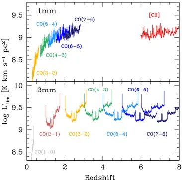
Figure1shows the redshift ranges and associated luminosity limits reached for various transitions in the two bands. The combination of band 3 and band 6 provides virtually complete CO redshift coverage. The luminosity limits are computed assuming 5σ significance, a line width of 200 km s−1, and unresolved emission at the angular resolution of our data. At z1.5, the luminosity limit (expressed as a velocity-integrated temperature over the beam, which is constant for all CO transitions in the case of thermalized emission) is roughly constant as a function of redshift for different CO transitions as well as for[CII]: ∼2×10⁹K km s−1pc2.
3. ANALYSIS
Given the blank-field approach of ASPECS, with no pre-selection on the targeted sources, we have a well-defined, volume-limited sample of galaxies at various redshifts where we can search for CO emission. We first concentrate on the “blind” CO detections presented in Table 2 of PaperI, and then include the information from galaxies with a known redshift. This provides us with direct constraints on the CO luminosity function in various redshift bins. We then use these constraints
to infer the CO(1–0) luminosity functions in various redshift bins, and therefore the H2 mass (MH2) budget in galaxies
throughout cosmic time.
3.1. CO Detections 3.1.1. Blind Detections
In PaperI, we describe our“blind search” for CO emission based purely on the ALMA data (i.e., with no support from ancillary data at other wavelengths).34 In brief, we perform a floating average of consecutive frequency channels in bins of ∼50–300 km s−1 in the imaged cubes. For each averaged
image, we compute the map rms and select peaks based on their signal-to-noise ratio (S/N). A search for negative (= noise) peaks allows us to quantify the fidelity of our line candidates based on their S/N, and the injection of mock lines allows us to assess the level of completeness of our search as a function of various line parameters, including the line luminosity. The final catalog consists of 10 line candidates from the 3 mm cube, and 11 from the 1 mm cube. We use a Gaussian fit of the candidate spectra to estimate the line flux, width, and frequency (see Table 2 of Paper I), and we
investigate the available optical/near-IR images to search for possible counterparts.
The line identification (and therefore the redshift association) requires a number of steps, similar to our earlier study of the Hubble Deep Field North(HDF-N, Decarli et al.2014), which
are as follows:
Figure 1. Redshift coverage and luminosity limit reached in our 1 mm and 3 mm scans, for various CO transitions and for the[CII] line. The (5σ) limits
plotted here are computed assuming point-source emission, and are based on the observed noise per channel, scaled for a line width of 200 km s−1. The combination of bands 3 and 6 offers a virtually complete CO redshift coverage. The luminosity limit(expressed as velocity-integrated temperature) is roughly constant at z1.5. The depth of our observations is sufficient to sample the typical knee of the expected CO luminosity functions (L′∼5× 10⁹ K km s−1pc2).
34
The code for the blind search of line candidates is publicly available at
(i) We inspect the cubes at the position of each line candidate, and search for multiple lines. If multiple lines are found, the redshift should be uniquely defined. Since
[ ( )] ( )
nCOJ- -J 1 »J nCO 1 0- , some ambiguity may still be in
place(e.g., two lines with a frequency ratio of 2 could be CO(2–1) and CO(4–3), or CO(3–2) and CO(6–5)). In these cases, the following steps allow us to break the degeneracy.
(ii) The absence of multiple lines can then be used to exclude some redshift identifications. For example, lines with similar J should show similar fluxes, under reasonable excitation conditions. If we identify a bright line as, e.g., CO(5–4), we expect to see a similarly luminous CO(4–3) line (if this falls within the coverage of our data set). If that is not the case, then we can exclude this line identification.
(iii) The exquisite depth of the available multi-wavelength data allows us to detect the starlight emission of galaxies with stellar mass M*∼108Meat almost all z<2. In the
absence of an optical/near-IR counterpart, we thus exclude redshift identification that would locate the source at z<2.
(iv) In the presence of an optical/near-IR counterpart, the line identification is guided by the availability of optical redshift estimates. Optical spectroscopy (e.g., see the compilations by Le Fèvre et al. 2005; Coe et al. 2006; Skelton et al. 2014; Morris et al. 2015) is considered
secure (typical uncertainties are of the order of a few hundred km s−1). When not available, we rely on Hubble Space Telescope (HST) grism data (Morris et al. 2015; Momcheva et al. 2016) or photometric redshifts (Coe
et al.2006; Skelton et al.2014).
Ten out of 21 blindly selected lines are uniquely identified in this way. A bootstrap analysis is then adopted to account for the remaining uncertainties in the line identification: to each source, we assign a redshift probability distribution that is proportional to the comoving volume in the redshift bins sampled with all the possible line identifications. We then run 1000 extractions of the redshift values picked from their probability distributions and compute the relevant quantities (line luminosities, inferred molecular masses, contribution to the cosmic density of molecular gas) in each case. The results are then averaged among all the realizations. The line identifications and associated redshifts are listed in Table1.
To compute the contribution of each line candidate to the CO luminosity functions and to the cosmic budget of molecular gas mass in galaxies, we need to account for the fidelity (i.e., the reliability of a line candidate against false-positive detections) and completeness(i.e., the fraction of line candidates that we retrieve as a function of various line parameters) of our search. For the fidelity, we infer the incidence of false-positive detections from the statistics of negative peaks in the cubes as a function of the line S/N, as described in Section3.1.1 of PaperI. Figure2shows the completeness of our line search as a function of the line luminosity. This is obtained by creating a sample of 2500 mock lines (as point sources), with a uniform distribution of frequency, peakflux density, width, and position within the primary beam. Under the assumption of observing a given transition (e.g., CO(3–2)), we convert the input frequency into redshift, and the integrated line flux ( Fline)
from the peak flux density and width. We then compute line
luminosities for all the mock input lines as
( ) ( ) n ¢ = ´ + - -⎜ ⎟ ⎛ ⎝ ⎞⎠ ⎛ ⎝ ⎜ ⎞ ⎠ ⎟ L z F D K km s pc 3.25 10 1 Jy km s GHz Mpc 1 1 2 7 3 line 1 obs 2 L 2
whereνobsis the observed frequency of the line and DLis the
luminosity distance(see, e.g., Solomon et al.1997). Finally, we
run our blind line search algorithm and display the fraction of retrieved-to-input lines as a function of the input line luminosity. Our analysis is 50% complete down to line luminosities of (4–6)×109K km s−1pc2 at 3 mm for any J>1, and (1–6)×108K km s−1pc2at 1 mm for any J>3, in the area corresponding to the primary beam of the 3 mm observations. The completeness distributions as a function of line luminosity in the J=1 case (at 3 mm) and the J=3 case (at 1 mm) show long tails toward lower luminosities due to the large variations of DLwithin our scans for these lines(see also
Figure1). The levels of fidelity and completeness at the S/N
and luminosity of the line candidates in our analysis are reported in Table1. At low S/N, flux-boosting might bias our results high, through effectively overestimating the impact of a few intrinsically bright sources against many fainter ones scattered above our detection threshold by the noise. However, the relatively high S/N (>5) of our line detections, and the statistiscal corrections for missed lines that are scattered below our detection threshold, and for spurious detections, make the impact offlux-boosting negligible in our analysis.
3.1.2. CO Line Stack
We can improve the sensitivity of our CO search beyond our “blind” CO detections by focusing on those galaxies where an accurate redshift is available via optical/near-IR spectroscopy. Slit spectroscopy typically leads to uncertainties of a few hundred km s−1, while grism spectra from the 3D-HST (Momcheva et al. 2016) have typical uncertainties of
∼1000 km s−1 due to the coarser resolution and poorer S/N.
By combining the available spectroscopy, we construct a list of 42 galaxies for which slit or grism redshift information is available(Le Fèvre et al.2005; Coe et al.2006; Skelton et al.
2014; Morris et al.2015; Momcheva et al.2016) within 37 5
from our pointing center (this corresponds to the area of the primary beam at the low-frequency end of the band 3 scan). Out of these, 36 galaxies have a redshift for which one or more J<5 CO transitions have been covered in our frequency scans. We extract the 3 mm and 1 mm spectra of all these sources, and we stack them with a weighted average. As weights, we used the inverse of the variance of the spectral noise. This is the pixel rms of each channel map, corrected a posteriori for the primary beam attenuation at the source position. As Figure3shows, no obvious line is detected above a S/N=3. If we integrate the signal over a 1000 km s−1wide bin centered on the rest-frame frequency of the lines, we retrieve a ∼2σ detection of the CO(2–1) and CO(4–3) lines (corresponding to average line fluxes of ∼0.006 Jy km s−1and
∼0.010 Jy km s−1 respectively). However, given their low
significance, and that they are drawn from a relatively sparse sample, we opt not to include them in the remainder of the analysis, until we are able to significantly expand the list of sources with secure optical/near-IR redshifts. This will be
possible thanks to the advent of integral field spectroscopy units with large field of view, such as MUSE, which will provide spectra (and therefore redshifts) for hundreds of galaxies in our pointing.
3.2. CO Luminosity Functions
The CO luminosity functions are constructed as follows:
( )
å
( ) F = = L V C log i 1 Fid 2 j N j j 1 iHere, Niis the number of galaxies with a CO luminosity falling
into the luminosity bin i, defined as the luminosity range betweenlogLi-0.5andlogLi+0.5, while V is the volume
of the universe sampled in a given transition. Each entry j is down-weighted according to the fidelity (Fidj) and up-scaled according to the completeness(Cj) of the jth line. As described in Paper I, the fidelity at a given S/N is defined as (Npos-Nneg) Npos, where Npos/neg is the number of positive
or negative lines with said S/N. This definition of the fidelity allows us to statistically subtract the false-positive line Table 1
Catalog of the Line Candidates Discovered with the Blind Line Search
ASPECS ID R.A. Decl. Fidelity C Counterpart? Notes Line zCO L′ MH2
Ident. (108K km s−1pc2) (108Me) (1) (2) (3) (4) (5) (6) (7) (8) (9) (10) (11) 3 mm 3 mm.1 03:32:38.52 −27:46:34.5 1.00 1.00 Y (i), (iv)(b) 3 2.5442 240.4±1.0 2061±9 3 mm.2 03:32:39.81 −27:46:11.6 1.00 1.00 Y (i), (iv)(a) 2 1.5490 136.7±2.1 648±10 3 mm.3 03:32:35.55 −27:46:25.7 1.00 0.85 Y (iv)(a) 2 1.3823 33.7±0.7 160±3 3 mm.4 03:32:40.64 −27:46:02.5 1.00 0.85 N (ii) 3 2.5733 45.8±1.0 393±9 4 4.0413 92.2±2.8 1071±33 5 5.3012 89.5±2.7 L 3 mm.5 03:32:35.48 −27:46:26.5 0.87 0.85 Y (iv)(a) 2 1.0876 28.3±0.9 134±4 3 mm.6 03:32:35.64 −27:45:57.6 0.86 0.85 N (ii), (iii) 3 2.4836 72.8±1.0 624±9 4 3.6445 77.3±1.0 898±12 5 4.8053 76.2±1.0 L 3 mm.7 03:32:39.26 −27:45:58.8 0.86 0.85 N (ii), (iii) 3 2.4340 25.9±1.0 222±9 4 3.5784 27.6±1.0 321±12 5 4.7227 27.3±1.0 L 3 mm.8 03:32:40.68 −27:46:12.1 0.76 0.85 N (ii), (iii) 3 2.4193 58.6±0.9 502±8 4 3.5589 62.6±1.0 727±12 5 4.6983 62.0±1.0 L 3 mm.9 03:32:36.01 −27:46:47.9 0.74 0.85 N (ii), (iii) 3 2.5256 30.5±1.0 261±9 4 3.7006 32.3±1.0 375±12 5 4.8754 31.8±1.0 L 3 mm.10 03:32:35.66 −27:45:56.8 0.61 0.85 Y (ii), iv(b) 3 2.3708 70.4±0.9 603±8 1 mm 1 mm.1a 03:32:38.54 −27:46:34.5 1.00 1.00 Y i, iv(b) 7 2.5439 48.02±0.37 L 1 mm.2a 03:32:38.54 −27:46:34.5 1.00 1.00 Y i, iv(a) 8 2.5450 51.42±0.23 L 1 mm.3 03:32:38.54 −27:46:31.3 0.93 0.85 Y iv(b) 3 0.5356 3.66±0.08 31±1 1 mm.4 03:32:37.36 −27:46:10.0 0.85 0.65 N i [CII] 6.3570 12.49±0.23 L 1 mm.5 03:32:38.59 −27:46:55.0 0.79 0.75 N (ii) 4 0.7377 12.95±0.09 150±1 [CII] 6.1632 31.84±0.22 L 1 mm.6 03:32:36.58 −27:46:50.1 0.78 0.75 Y iv(c) 4 1.0716 21.45±0.15 249±2 5 1.5894 29.12±0.21 L 6 2.1070 33.68±0.24 L 1 mm.7 03:32:37.91 −27:46:57.0 0.77 1.00 N (ii), (iii) 4 0.7936 37.53±0.10 436±1 [CII] 6.3939 84.01±0.23 L 1 mm.8 03:32:37.68 −27:46:52.6 0.71 0.72 N (ii), (iii) [CII] 7.5524 23.22±0.24 L 1 mm.9 03:32:36.14 −27:46:37.0 0.63 0.75 N (ii), (iii) 4 0.8509 8.21±0.12 95±1 [CII] 6.6301 16.84±0.25 L 1 mm.10 03:32:37.08 −27:46:19.9 0.62 0.75 N (ii), (iii) 4 0.9442 14.74±0.18 171±2 6 1.9160 25.05±0.30 L [CII] 7.0147 26.59±0.32 L 1 mm.11 03:32:37.71 −27:46:41.0 0.61 0.85 N (ii), (iii) 3 0.5502 4.84±0.09 41±1 [CII] 7.5201 16.25±0.30 L Note. (1) Line ID. (2, 3) R.A. and decl. (J2000). (4) Fidelity level at the S/N of the line candidate. (5) Completeness at the luminosity of the line candidate. (6) Is there an optical/near-IR counterpart? (7) Notes on line identification: (i) multiple lines detected in the ASPECS cubes; (ii) lack of other lines in the ASPECS cubes; (iii) absence of optical/near-IR counterpart suggests high z; (iv) supported by (a) spectroscopic, (b) grism, or (c) photometric redshift. (8) Possible line identification: a cardinal number indicates the upper J level of a CO transition. (9) CO redshift corresponding to the adopted line identification. (10) Line luminosity, assuming the line identification in column (8). The uncertainties are propagated from the uncertainties in the line flux measurement. (11) Molecular gas mass MH2as derived from the
observed CO luminosity(see Equation (4)), only for J<5 CO lines. a
candidates from our blind selection. The uncertainties on
( )
F logLi are set by the Poissonian errors on Ni, according to
Gehrels (1986).35 We consider the confidence level corresp-onding to 1σ. We include the uncertainties associated with the line identification and the errors from the flux measurements in the bootstrap analysis described in Section3.1.1. Given that all our blind sources have S/N>5 by construction, and the number of entries is typically a few sources per bin, Poissonian uncertainties always dominate. The results of the bootstrap are averaged in order to produce the final luminosity functions.
The CO luminosity functions obtained in this way are shown in Figure4. For comparison, we include the predictions based on semi-analytical models by Lagos et al.(2012) and Popping
et al. (2016) and on the empirical IR luminosity function of
Herschel sources by Vallini et al. (2016), as well as the
constraints obtained by the earlier study of the HDF-N(Walter et al.2014). Our observations reach the knee of the luminosity
functions in almost all redshift bins. The only exception is the CO(4–3) transition in the á ñ =z 3.80 bin, for which the models by Lagos et al.(2012) place the knee approximately one order
of magnitude below that predicted by Popping et al. (2016),
thus highlighting the large uncertainties in the state-of-the-art predictions of gas content and CO excitation, especially at high redshift. In particular, these two approaches differ in the treatment of the radiative transfer and CO excitation in a number of ways:(1) Lagos et al. (2012) adopt a single value of
gas density for each galaxy, whereas Popping et al. (2016)
construct a density distribution for each galaxy, and assume a log-normal density distribution for the gas within clouds; (2) Lagos et al.(2012) include heating from both UV and X-rays
Figure 2. Luminosity limit reached in our 3 mm and 1 mm scans, for various CO transitions. The completeness is computed as the number of mock lines retrieved by our blind search analysis divided by the number of input mock lines, and here it is plotted as a function of the line luminosity. The 50% limits, marked as dashed vertical lines, are typically met at L′=(3–6)×109K km s−1pc2
at 3 mm for any J>1, and at L′=(4–8)×108K km s−1pc2
at 1 mm for any J>3. The J=1 and 3 cases in the 3 mm and 1 mm cubes show a broader distribution toward lower luminosity limits due to the wide spread of luminosity distance for these transitions within the frequency ranges of our observations.
Figure 3. Stacked millimeter spectrum of the sources in our field with optical/ near-IR redshifts. The adopted spectral bin is 70 km s−1 wide. The 1σ uncertainties are shown as gray lines. We highlight the±500 km s−1range where the stackedflux is integrated. We also list the number of sources entering each stack. No clear detection is reported in any of the stacked transitions.
35
According to Cameron(2011), the binomial confidence intervals in Gehrels
(1986) might be overestimated in the low-statistics regime compared to a fully
Bayesian treatment of the distributions. A similar effect is possibly in place for Poissonian distributions, although a formal derivation is beyond the scope of this work. Here we conservatively opt to follow the classical method of Gehrels(1986).
(although the latter might be less critical for the purposes of this paper), while Popping et al. (2016) consider only the UV
contribution to the heating;(3) the CO chemistry in Lagos et al. (2012) is set following the UCL_PDR photodissociation
region code (Bell et al. 2006, 2007), and in Popping et al.
(2016) it is based on a fit to results from the photodissociation
region code of Wolfire et al. (2010); (4) the CO excitation in
Lagos et al.(2012) is also based on the UCL_PDR code, while
Popping et al. (2016) adopt a customized escape probability
code for the level population;(5) the typical αCOin the models
of Lagos et al.(2012) is higher than in Popping et al. (2016),
although the exact value ofαCOin both models changes from
galaxy to galaxy(i.e., the CO(1–0) luminosity functions do not translate into H2mass functions with a simple scaling).
Our observations shown in Figure 4indicate that an excess of CO-bright sources with respect to semi-analytical models might be in place. This is apparent in the 3 mm data. However, the same excess is not observed in the 1 mm band. In particular, in the á ñ =z 1.43 bin, the lack of bright CO(5–4) lines (compared with the brighter CO(2–1) emission reported here) suggests that the CO excitation is typically modest.
Such apparent low CO excitation is supported by the detailed analysis of a few CO-bright sources presented in a companion paper (Paper IV of this series, Decarli et al. 2016b). These
findings guide our choice of a low-excitation template to convert the observed J>1 luminosities into CO(1–0). In the
next steps of our analysis, we refer to the template of CO excitation of main-sequence galaxies by Daddi et al.(2015): if
rJ1is the temperature ratio between the CO( J–[J – 1]) and the
CO(1–0) transitions, we adopt rJ1= 0.76±0.09, 0.42±0.07,
0.23±0.04 for J=2, 3, 5. In the case of CO(4–3) (which is not part of the template), we interpolate the models shown in the left-hand panel of Figure10 in Daddi et al. (2015), yielding
r41 = 0.31±0.06, where we conservatively assume a 20%
uncertainty. Each line luminosity is then converted into CO (1–0) according to
( )
( ) ( [ ])
¢ - = ¢ - -
-L L r
log CO 1 0 log COJ J 1 log J1. 3 The uncertainties in the excitation correction are included in the bootstrap analysis described in Section 3.1.1. Based on these measurements, we derive CO(1–0) luminosity functions following Equation (2). The results are shown in Figure 5. Compared with Figure4, we have removed the á ñ =z 1.43 bin from the 1 mm data because the CO(2–1) line at 3 mm is observed in practically the same redshift range and is subject to smaller uncertainties related to CO excitation corrections. Our observations succeed in sampling the predicted knee of the CO (1–0) luminosity functions at least up to z∼3. Our measure-ments reveal that the knee of the CO(1–0) luminosity function shifts toward higher luminosities as we move from z≈0 (Keres et al. 2003; Boselli et al. 2014) to z∼2. Our results
agree with the model predictions at z<1. However, at z>1 they suggest an excess of CO-luminous sources compared with the current models. This result is robust against uncertainties in CO excitation. For example, it is already apparent in the á ñ =z 1.43 bin, where we covered the CO(2–1) line in our 3 mm cube; this line is typically close to being thermalized in star-forming galaxies, so excitation corrections are small. Our result is also broadly consistent with thefindings by Keating et al. (2016), based on a CO(1–0) intensity mapping study at
z=2–3, which is unaffected by CO excitation. 3.3. Cosmic H2Mass Density
To derive H2 masses, and the evolution of the cosmic H2
mass density, we now convert the CO(1–0) luminosities into molecular gas masses MH2:
( )
( ) a
= ¢
-MH2 COLCO 1 0. 4
The conversion factor αCO implicitly assumes that CO is
optically thick. The value of αCO depends critically on the
metallicity of the interstellar medium (see Bolatto et al.
2013 for a review). A galactic value αCO=3–6 Me
(K km s−1pc2)−1 is expected for most non-starbursting
galaxies with metallicities Z0.5 Ze (Wolfire et al. 2010;
Glover & Mac Low2011; Feldmann et al.2012). At z∼0.1,
this is the case for the majority of main-sequence galaxies with M*>109Me(Tremonti et al.2004). This seems to hold even
at z∼3, if one takes into account the SFR dependence of the mass–metallicity relation (Mannucci et al. 2010). Following
Daddi et al. (2010a), we thus assume αCO=3.6 Me
(K km s−1pc2)−1for all the sources in our sample. In Section4
we discuss how our results would be affected by relaxing this assumption.
Figure 4. CO luminosity functions in various redshift bins. The constraints from our ALMA UDF project are marked as red squares, with the vertical size of the box showing the Poissonian uncertainties. The results of the HDF study by Walter et al.(2014) are shown as cyan boxes, with error bars marking the
Poissonian uncertainties. Semi-analytical models by Lagos et al.(2012) and
Popping et al. (2016) as well as the empirical predictions by Vallini et al.
(2016) are shown for comparison. Our ALMA observations reach the depth
required to sample the expected knee of the luminosity functions in most cases (the only exception being the á ñ =z 3.80 bin when compared with the predictions by Lagos et al.2012). Our observations reveal an excess of
CO-luminous sources at the bright end of the luminosity function, especially in the 3 mm survey, with respect to the predictions. Such an excess is not observed in the 1 mm survey, suggesting that the CO excitation is typically modest compared with the models shown here.
Figure 5. CO(1–0) luminosity functions in various redshift bins. The constraints from ASPECS are marked as red squares, with the vertical size of each box showing the uncertainties. The results from the 3 mm scan with PdBI by Walter et al.(2014) are shown as cyan boxes, with error bars marking the Poissonian uncertainties. The
observed CO(1–0) luminosity functions of local galaxies by Keres et al. (2003) and Boselli et al. (2014) are shown as red circles and orange diamonds in the first
panel, respectively, and as gray points for comparison in all the other panels. The intensity mapping constraints from Keating et al.(2016) are shown as a shaded
yellow area. Semi-analytical models by Lagos et al.(2012) and Popping et al. (2016) as well as the empirical predictions by Vallini et al. (2016) are shown for
comparison. The scale for mass function shown at the top assumes afixed αCO=3.6 Me(K km s−1pc2)−1. Our results agree with the predictions at z<1 and
suggest that an excess of bright sources with respect to both the empirical predictions by Vallini et al.(2016) and the models by Lagos et al. (2012) appears at z>1.
Figure 6. Comoving cosmic mass density of molecular gas in galaxies ρ(H2) as a function of redshift, based on our molecular survey in the UDF. Our ASPECS
constraints are displayed as red boxes. The vertical size indicates our uncertainties(see text for details). Our measurements are not extrapolated to account for the faint end of the molecular gas mass function. Since our observations sample the expected knee of the CO luminosity functions in the redshift bins of interest, the correction is expected to be small(<2×). Semi-analytical model predictions by Obreschkow et al. (2009), Obreschkow & Rawlings (2009), Lagos et al. (2012), and Popping
et al.(2014a,2014b) are shown as lines; the empirical predictions by Sargent et al. (2014) are plotted as a gray area; the constraints by Keating et al. (2016) are
displayed with triangles; the PdBI constraints(Walter et al.2014) are represented by cyan boxes. Our ALMA observations show an evolution in the cosmic density of
molecular gas up to z∼4.5. The global molecular content of galaxies at the peak of galaxy formation appears 3–10 times higher than in galaxies in the local universe, although large uncertainties remain due to the limited area that is covered.
Next, we compute the cosmic density of molecular gas in galaxies, ρ(H2): ( )
åå
( ) r = = V M P C H 1 5 i j N i j j j 2 1 , iwhere Mi j, is a compact notation for MH2of the jth galaxy in
mass bin i, and the index i cycles over all the mass bins. As for Φ, the uncertainties on ρ(H2) are dominated by the Poissonian
errors. Ourfindings are shown in Figure6and are summarized in Table2. We note that the measurements presented here are based on only the observed part of the luminosity function. Therefore, we do not attempt to correct for undetected galaxies in lower luminosity bins given the large uncertainties in the individual luminosity bins and the unknown intrinsic shape of the CO luminosity function.
From Figure 6, it is clear that there is an evolution in the molecular gas content of galaxies with redshift, in particular compared with the z=0 measurements by Keres et al. (2003)
(ρ(H2)=(2.2±0.8)×107MeMpc−3) and Boselli et al.
(2014) (ρ(H2)=(1.2±0.2)×107MeMpc−3). The global
amount of molecular gas stored in galaxies at the peak epoch of galaxy assembly is 3–10 times larger than at the present day. This evolution can be followed up to z∼4.5, i.e., 90% of the age of the universe. This trend agrees with the initial findings using PdBI(Walter et al.2014). Our results are consistent with
the constraints on ρ(H2) at z∼2.6 based on the CO(1–0)
intensity mapping experiment by Keating et al. (2016)36: by assuming a linear relation between the CO luminosity of galaxies and their dark matter halo mass, they interpret their constraint on the CO power spectrum in terms of ρ (H2)<2.6×10
8
MeMpc−1 (at 1σ). They further tighten the
constraint onρ(H2) by assuming that the relation between LCO
and dark matter halo mass has a scatter of 0.37 dex (a factor≈2.3), which translates into ρ(H2)=1.1-+0.40.7 ´108
MeMpc−1, in excellent agreement with our measurement.
Ourfindings are also consistent with the global increase in the gas fraction as a function of redshift found in targeted observations (e.g., Daddi et al. 2010a; Genzel et al. 2010,
2015; Riechers et al. 2010; Tacconi et al. 2010,2013; Geach et al.2011; Magdis et al.2012; Magnelli et al.2012), although
wefind a large variety in the gas fraction in individual sources (see Paper IV Decarli et al. 2016b). Our results are also in
general agreement with the expectations from semi-analytical models (Obreschkow et al. 2009; Obreschkow & Rawlings
2009; Lagos et al. 2011,2012; Popping et al.2014a,2014b)
and from empirical predictions (Sargent et al. 2012, 2014).
From the present data, there is an indication for a decrease inρ (H2) at z>3, as suggested by some models.37A larger sample
of z>3 CO emitters with spectroscopically confirmed redshifts, and covering more cosmic volume, is required in order to explore this redshift range.
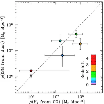
3.4. Estimates from Dust Continuum Emission In Figure 7 we compare the constraints on ρ(H2) inferred
from CO with those on ρ(ISM) derived from the dust continuum in our observations of the UDF. These are derived following Scoville et al. (2014). In brief, for each 1 mm
continuum source(see PaperII, Aravena et al.2016a), the ISM
mass is computed as ( ) ( ) n = + G G n -⎜ ⎟ ⎛ ⎝ ⎞⎠ ⎛ ⎝ ⎜ ⎞ ⎠ ⎟ M M z S D 10 1.78 1 mJy 350 GHz Gpc 6 ISM 10 4.8 3.8 0 RJ L 2
where Sν is the observed continuum flux density, ν is the
observing frequency(here, we adopt ν=242 GHz as the central frequency of the continuum image), ΓRJis a unitless correction
factor that accounts for the deviation from theν2scaling of the Rayleigh–Jeans tail, Γ0=0.71 is the tuning value obtained at
lowz, and DL is the luminosity distance (see Equation(12) in
Scoville et al. 2014). The dust temperature (implicit in the
definition of ΓRJ) is set to 25 K. The ISM masses obtained via
Equation (6) for each galaxy detected in the continuum (see
Paper II, Aravena et al. 2016a) are then split into the same
redshift bins used for the CO-based estimates and summed. We include here all the sources detected down to S/N=3 in the 1 mm continuum. Poissonian uncertainties are found again to dominate the estimates of ρ (if model uncertainties are neglected). The values of ρ(ISM) obtained in this way are reported in Table 2. Wefind that the estimates of ISM mass density are roughly consistent (within the admittedly large uncertainties) with the CO-based estimates in the lower redshift Table 2
Redshift Ranges Covered in the Molecular Line Scans, the Corresponding Comoving Volume, the Number of Galaxies in each Bin(Accounting for Different Line Identifications), and Our Constraints on the Molecular Gas Content in Galaxies ρ(H2) and ρ(ISM)
Transition ν0 zmin zmax á ñz Volume N(H2) logρmin(H2) logρmax(H2) N(ISM) logρmin(ISM) logρmax(ISM)
(GHz) (Mpc3) (M eMpc−3) (MeMpc−3) (MeMpc−3) (MeMpc−3) (1) (2) (3) (4) (5) (6) (7) (8) (9) (10) (11) (12) 1 mm(212.032–272.001 GHz) CO(3–2) 345.796 0.2713 0.6309 0.4858 314 1–2 6.56 7.76 2 6.36 7.18 CO(4–3) 461.041 0.6950 1.1744 0.9543 1028 0–5 6.83 7.73 5 7.13 7.60 3 mm(84.176–114.928 GHz) CO(2–1) 230.538 1.0059 1.7387 1.4277 1920 3 7.53 8.09 13 7.50 7.77 CO(3–2) 345.796 2.0088 3.1080 2.6129 3363 2–7 7.69 8.28 6 7.04 7.46 CO(4–3) 461.041 3.0115 4.4771 3.8030 4149 0–5 5.53 7.58 0 L 6.21
36For a CO intensity mapping experiment based on the ASPECS data, see
Carilli et al.(2016).
37
Theρ(H2) value at z>3 in the models by Popping et al. (2016) is lower
than in the predictions in Lagos et al.(2011). This might be surprising because
the CO(1–0) luminosity function in the former exceeds that in the latter, especially at high redshift(see Figure5). This discrepancy is explained with the
bins (z∼0.5, 0.95, and 1.4), while discrepancies are found at z>2, where ρ(H2) estimates based on CO tend to be larger than
ρ(ISM) estimates based on dust. Scoville et al. (2016) present a
different calibration of the recipe that would shift the dust-based mass estimates up by a factor 1.5. However, even applying the more recent calibration would not be sufficient to significantly mitigate the discrepancy between CO-based and dust-based estimates of the gas mass at high redshift. In PaperII(Aravena
et al.2016a) we show that all of our 1 mm continuum sources
detected at>3.5σ (except one) are at z<2. On the other hand, the redshift distribution of CO-detected galaxies in our sample extends well beyond z = 2, thus leading to the discrepancy in the ρ estimates at high redshift. Possible explanations for this difference might be related to the dust temperature and opacity, and to the adopted αCO. A higher dust temperature in high-z
galaxies (>40 K) would shift the dust emission toward higher frequencies, thus explaining the comparably lower dust emission observed at 1 mm(at a fixed IR luminosity). Moreover, at z=4 our 1 mm continuum observations sample the rest-frame ∼250 μm range, where dust might turn optically thick (thus leading to underestimates of the dust emission). Finally, we might be overestimating molecular gas masses at high z if the αCO factor is typically closer to the ULIRG/starburst value
(αCO≈0.8 Me(K km s−1pc2)−1, see Daddi et al. 2010b;
Bolatto et al. 2013). However, the observed low CO excitation
and faint IR luminosity do not support the ULIRG scenario for our high-z galaxies. Furthermore, any metallicity evolution would yield a higherαCOat high z, instead of a lower one. In
Paper IV we discuss the discrepancy between dust- and CO-based gas masses on a source-by-source basis.
4. SUMMARY AND DISCUSSION
In this paper we use our ALMA molecular scans of the Hubble UDF in band3 and band6 to place blind constraints on the CO luminosity function up to z∼4.5. We provide constraints on the evolution of the cosmic molecular gas density as a function of redshift. This study is based on galaxies that have been blindly selected through their CO emission, and not through any other multi-wavelength property. The CO number counts have been corrected for by using two parameters,fidelity and completeness, which take into account the number of false-positive detections due to noise peaks and the fraction of lines that our algorithm successfully recovers in our data cubes from a parent population of known (artificial) lines.
We start by constructing CO luminosity functions for the respective rotational transitions of CO for both the 3 mm and 1 mm observations. We compare these measurements with models that also predict CO luminosities in various rotational transitions, i.e., no assumptions were made in comparing our measurements with the models. This comparison shows that our derived CO luminosity functions lie above the predictions in the 3 mm band. On the other hand, in the 1 mm band our measurements are comparable to the models. Together this implies that the observed galaxies are more gas-rich than currently accounted for in the models, but with lower excitation.
Accounting for a CO excitation characteristic of main-sequence galaxies at z∼1–2, we derive the CO luminosity function of the ground-state transition of CO( J = 1–0) from our observations. We do so only up to the J=4 transition of CO, to ensure that our results are not too strongly affected by the excitation corrections that would dominate the analysis at higher J. We find an evolution in the CO(1–0) luminosity function compared with observations in the local universe, with an excess of CO-emitting sources at the bright end of the luminosity functions. This is in general agreement with first constraints on the CO intensity mapping from the literature. This evolution exceeds what is predicted by the current models. This discrepancy appears to be a common trait of models of galaxy formation: galaxies with M*>1010Meat z=2–3 are
predicted to be 2–3 times less star-forming than observed (see, e.g., the recent review by Somerville & Davé 2015), and
similarly less gas-rich(see the analysis in Popping et al.2015a,
2015b).
The sensitivity of the ALMA observations reaches below the knee of the predicted CO luminosity functions (around 5×10⁹K km s−1pc2) at all redshifts. We convert our luminosity measurements into molecular gas masses via a “Galactic” conversion factor. By summing the molecular gas masses obtained at each redshift, we obtain an estimate of the cosmic density of molecular gas in galaxies,ρ(H2). Given the
admittedly large uncertainties (mainly due to Poisson errors), and the unknown shape of the intrinsic CO luminosity functions, we do not extrapolate our measurements outside the range of CO luminosities(i.e., H2masses) covered in our
survey.
We find an increase (by a factor of 3–10) in the cosmic density of molecular gas from z∼0 to z∼2–3, albeit with large uncertainties given the limited statistics. This is consistent with previousfindings that the gas mass fraction increases with redshift (see, e.g., Tacconi et al. 2010, 2013; Magdis et al.
2012). However, our measurements have been derived in a
Figure 7. Comparison between the CO-derived estimates of ρ(H2) and the
1 mm dust continuum-based estimates ofρ(ISM). The galaxies are binned in the same redshift bins as presented in Figure6, as indicated by the color of the symbols. The one-to-one case is shown as a dashed line. The dust-based estimates agree with the CO-based estimates at z<2, but they seem to fall below this line at higher redshifts.
completely different fashion, by simply counting the molecular gas that is present in a given cosmic volume, without any prior knowledge of the general galaxy population in thefield. In this respect, our constraints on ρ(H2) are actually lower limits, in
the sense that they do not recover the full extent of the luminosity function. However,(a) we do sample the predicted knee of the luminosity function in most of the redshift bins, suggesting that we recover a large part(>50%) of the total CO luminosity per comoving volume; (b) the fraction of the CO luminosity function missed because of our sensitivity cut is likely larger at higher redshift, i.e., correcting for the contribution of the faint end would make the evolution in ρ (H2) even steeper.
We have also derived the molecular gas densities using the dust emission as a tracer for the molecular gas, following Scoville et al. (2014, 2016). The molecular gas densities
derived from dust emission are generally smaller than but broadly consistent with those measured from CO at z<2, but they might fall short at reproducing the predicted gas mass content of galaxies at z>2.
Our analysis demonstrates that CO-based estimates of gas mass result in 3–10 times higher gas masses in galaxies at z∼2 than in the local universe. The history of cosmic SFR (Madau & Dickinson2014) appears to at least partially follow
the evolution in molecular gas supply in galaxies. The remaining difference between the evolution of the SFR density (a factor of ∼20) and that of molecular gas (a factor of 3–10) may be due to the shortened depletion timescales. A further contribution to this difference may be ascribed to cosmic variance. The UDF in general (and therefore also the region studied here) is found to be underdense at z>3 (e.g., Figure14 in Beckwith et al. 2006) and in IR-bright sources
(Weiß et al. 2009). The impact of cosmic variance can be
estimated empirically from the comparison with the number counts of sources detected in the dust continuum (Aravena et al. 2016a), or analytically from the variance in the dark
matter structures, coupled with the clustering bias of a given galaxy population (see, e.g., Somerville et al.2004). Trenti &
Stiavelli (2008) provide estimates of the cosmic variance as a
function of field size, halo occupation fraction, survey completeness, and number of sources in a sample. For a Δz=1 bin centered at z = 2.5, a 100% halo occupation fraction, andfive sources detected over 1 arcmin2(i.e., roughly mimicking the z∼2.5 bin in our analysis), the fractional uncertainty in the number counts due to cosmic variance is ∼20% (∼60% if we include Poissonian fluctuations). Already an increase in target area by a factor of 5(resulting in a field that is approximately the size of the Hubble eXtremely Deep Field, Illingworth et al. 2013), at similar depth, would
beat down the uncertainties significantly (30%, including Poissonian fluctuations). With ALMA now being fully operational, such an increase in areal coverage appears to be within reach.
We thank the anonymous referee for excellent feedback that improved the quality of the paper. F.W., I.R.S., and R.J.I. acknowledge support through ERC grants COSMIC-DAWN, DUSTYGAL, and COSMICISM, respectively. M.A. acknowl-edges partial support from FONDECYT through grant 1140099. D.R. acknowledges support from the National Science Foundation under grant number AST-1614213 to Cornell University. F.E.B. and L.I. acknowledge Conicyt
grants Basal-CATA PFB-06/2007 and Anilo ACT1417. F.E.B. also acknowledges support from FONDECYT Regular 1141218(FEB), and the Ministry of Economy, Development, and Tourism’s Millennium Science Initiative through grant IC120009, awarded to The Millennium Institute of Astro-physics, MAS. I.R.S. also acknowledges support from STFC (ST/L00075X/1) and a Royal Society/Wolfson Merit award. Support for R.D. and B.M. was provided by the DFG priority program 1573“The physics of the interstellar medium.” A.K. and F.B. acknowledge support by the Collaborative Research Council 956, sub-project A1, funded by the Deutsche Forschungsgemeinschaft (DFG). L.I. acknowledges Conicyt grants Basal-CATA PFB-06/2007 and Anilo ACT1417. R.J.A. was supported by FONDECYT grant number 1151408. This paper makes use of the following ALMA data: [ADS/JAO. ALMA# 2013.1.00146.S and 2013.1.00718.S.]. ALMA is a
partnership of ESO (representing its member states), NSF (USA), and NINS (Japan), together with NRC (Canada), NSC and ASIAA (Taiwan), and KASI (Republic of Korea), in cooperation with the Republic of Chile. The Joint ALMA Observatory is operated by ESO, AUI/NRAO, and NAOJ. The 3 mm part of the ASPECS project had been supported by the German ARC.
REFERENCES
Aravena, M., Decarli, R., Walter, F., et al. 2016a,ApJ, 833, 68(Paper II) Beckwith, S. V., Stiavelli, M., Koekemoer, A. M., et al. 2006,AJ,132, 1729
Bell, T. A., Roueff, E., Viti, S., & Williams, D. A. 2006,MNRAS,371, 1865
Bell, T. A., Viti, S., & Williams, D. A. 2007,MNRAS,378, 983
Blitz, L., & Rosolowsky, E. 2006,ApJ,650, 933
Bolatto, A. D., Warren, S. R., Leroy, A. K., et al. 2015,ApJ,809, 175
Bolatto, A. D., Wolfire, M., & Leroy, A. K. 2013,ARA&A,51, 207
Boselli, A., Cortese, L., Boquien, M., et al. 2014,A&A,564, A66
Bothwell, M. S., Smail, I., Chapman, S. C., et al. 2013,MNRAS,429, 3047
Cameron, E. 2011,PASA,28, 128
Carilli, C. L., Chluba, J., Decarli, R., et al. 2016,ApJ, 833, 73(Paper VII) Carilli, C. L., & Walter, F. 2013,ARA&A,51, 105
Casey, C. M., Narayanan, D., & Cooray, A. 2014, PhRv, 541, 45 Coe, D., Benítez, N., Sánchez, S. F., et al. 2006,AJ,132, 926
Crighton, N. H. M., Murphy, M. T., Prochaska, J. X., et al. 2015,MNRAS,
452, 217
da Cunha, E., Walter, F., Decarli, R., et al. 2013,ApJ,765, 9
Daddi, E., Bournaud, F., Walter, F., et al. 2010a,ApJ,713, 686
Daddi, E., Dannerbauer, H., Liu, D., et al. 2015,A&A,577, 46
Daddi, E., Elbaz, D., Walter, F., et al. 2010b,ApJL,714, L118
Decarli, R., Walter, F., Aravena, M., et al. 2016b,ApJ, 833, 70(Paper IV) Decarli, R., Walter, F., Carilli, C., et al. 2014,ApJ,782, 78
Feldmann, R., Gnedin, N. Y., & Kravtsov, A. V. 2012,ApJ,758, 127
Geach, J. E., Smail, I., Moran, S. M., et al. 2011,ApJL,730, L19
Gehrels, N. 1986,ApJ,303, 336
Genzel, R., Tacconi, L. J., Gracia-Carpio, J., et al. 2010,MNRAS,407, 2091
Genzel, R., Tacconi, L. J., Lutz, D., et al. 2015,ApJ,800, 20
Glover, S. C. O., & Mac Low, M.-M. 2011,MNRAS,412, 337
Gnedin, N. Y., & Kravtsov, A. V. 2010,ApJ,714, 287
Gnedin, N. Y., & Kravtsov, A. V. 2011,ApJ,728, 88
Griffen, B. F., Ji, A. P., Dooley, G. A., et al. 2016,ApJ,818, 10
Groves, B. A., Schinnerer, E., Leroy, A., et al. 2015,ApJ,799, 96
Gruppioni, C., Pozzi, F., Rodighiero, G., et al. 2013,MNRAS,432, 23
Illingworth, G. D., Magee, D., Oesch, P. A., et al. 2013,ApJS,209, 6
Keating, G. K., Marrone, D. P., Bower, G. C., et al. 2016,ApJ,830, 34
Keres, D., Yun, M. S., & Young, J. S. 2003,ApJ,582, 659
Krumholz, M. R., McKee, C. F., & Tumlinson, J. 2008,ApJ,689, 865
Krumholz, M. R., McKee, C. F., & Tumlinson, J. 2009,ApJ,693, 216
Lagos, C. d. P., Baugh, C. M., Lacey, C. G., et al. 2011,MNRAS,418, 1649
Lagos, C. d. P., Baugh, C. M., Zwaan, M. A., et al. 2014,MNRAS,440, 920
Lagos, C. d. P., Bayet, E., Baugh, C. M., et al. 2012,MNRAS,426, 2142
Le Fèvre, O., Vettolani, G., Garilli, B., et al. 2005,A&A,439, 845
Lilly, S. J., Tresse, L., Hammer, F., Crampton, D., & Le Fèvre, O. 1995,ApJ,
455, 108
Madau, P., Ferguson, H. C., Dickinson, M. E., et al. 1996,MNRAS,283, 1388
Magdis, G. E., Daddi, E., Elbaz, D., et al. 2011,ApJL,740, L15
Magdis, G. E., Daddi, E., Sargent, M., et al. 2012,ApJL,758, L9
Magnelli, B., Popesso, P., Berta, S., et al. 2013,A&A,553, 132
Magnelli, B., Saintonge, A., Lutz, D., et al. 2012,A&A,548, 22
Mannucci, F., Cresci, G., Maiolino, R., Marconi, A., & Gnerucci, A. 2010,
MNRAS,408, 2115
Momcheva, I. G., Brammer, G. B., van Dokkum, P. G., et al. 2016,ApJS,225, 27
Morris, A. M., Kocevski, D. D., Trump, J. R., et al. 2015,AJ,149, 178
Obreschkow, D., Heywood, I., Klöckner, H.-R., & Rawlings, S. 2009,ApJ,
702, 1321
Obreschkow, D., & Rawlings, S. 2009,ApJL,696, L129
Planck Collaboration XIII 2016,A&A,594A, 13
Popping, G., Behroozi, P. S., & Peeples, M. S. 2015,MNRAS,449, 477
Popping, G., Caputi, K. I., Trager, S. C., et al. 2015,MNRAS,454, 2258
Popping, G., Pérez-Beaupuits, J. P., Spaans, M., Trager, S. C., & Somerville, R. S. 2014a,MNRAS,444, 1301
Popping, G., Somerville, R. S., & Trager, S. C. 2014b,MNRAS,442, 2398
Popping, G., van Kampen, E., Decarli, R., et al. 2016, arXiv:1602.02761
Riechers, D. A., Carilli, C. L., Walter, F., & Momjian, E. 2010, ApJL,
724, L153
Riechers, D. A., Hodge, J., Walter, F., Carilli, C. L., & Bertoldi, F. 2011,ApJL,
739, L31
Rodighiero, G., Daddi, E., Baronchelli, I., et al. 2011,ApJL,739, L40
Sargent, M. T., Béthermin, M., Daddi, E., & Elbaz, D. 2012, ApJL, 747, L31
Sargent, M. T., Daddi, E., Béthermin, M., et al. 2014,ApJ,793, 19
Scoville, N., Aussel, H., Sheth, K., et al. 2014,ApJ,783, 84
Scoville, N., Sheth, K., Aussel, H., et al. 2016,ApJ,820, 83
Skelton, R. E., Whitaker, K. E., Momcheva, I. G., et al. 2014,ApJS,214, 24
Solomon, P. M., Downes, D., Radford, S. J. E., & Barrett, J. W. 1997,ApJ,
478, 144
Somerville, R. S., & Davé, R. 2015,ARA&A,53, 51
Somerville, R. S., Lee, K., Ferguson, H. C., et al. 2004,ApJL,600, L171
Spilker, J. S., Marrone, D. P., Aguirre, J. E., et al. 2014,ApJ,785, 149
Tacconi, L. J., Genzel, R., Neri, R., et al. 2010,Natur,463, 781
Tacconi, L. J., Neri, R., Genzel, R., et al. 2013,ApJ,768, 74
Tremonti, C. A., Heckman, T. M., Kauffmann, G., et al. 2004,ApJ,613, 898
Trenti, M., & Stiavelli, M. 2008,ApJ,676, 767
Vallini, L., Gruppioni, C., Pozzi, F., Vignali, C., & Zamorani, G. 2016,
MNRAS,456, L40
Walter, F., Decarli, R., Aravena, M., et al. 2016,ApJ, 833, 67(Paper I) Walter, F., Decarli, R., Sargent, M., et al. 2014,ApJ,782, 79
Weiß, A., Downes, D., Walter, F., & Henkel, C. 2007, ASPC,375, 25
Weiß, A., Kovács, A., Coppin, K., et al. 2009,ApJ,707, 1201