Alma Mater Studiorum – Università di Bologna
DOTTORATO DI RICERCA IN
INGEGNERIA, CIVILE, CHIMICA, AMBIENTALE E DEI MATERIALI
Ciclo XXIX°
Settore Concorsuale di afferenza: 08/A2
Settore Scientifico disciplinare: ICAR/03
TITOLO TESI
Modeling to manage activated sludge wastewater treatment
plant and facultative lagoons finishing for irrigation reuse
Presentata da: CARMINE FIORENTINO
Coordinatore Dottorato
Relatore
PROF. LUCA VITTUARI
PROF. MAURIZIO MANCINI
Co-Relatore
ING. LUCA LUCCARINI
2
Summary
List of Figures ... 6 List of Tables ... 9 List of symbols ... 12 List of abbreviations ... 13 Chapter 1. Introduction ... 141.1 Background and problem definition ... 14
1.2 Aim of the thesis and methodology ... 16
1.3 Publications and conference contributions ... 18
Section 1 THEORETICAL FRAMEWORK ... 20
Chapter 2. Water and wastewater reuse regulations ... 21
Chapter 3. The Activated Sludge process and its modeling ... 27
3.1 Mathematical modeling overview ... 27
3.2 Activated Sludge process: historical perspective ... 29
3.3 The Ludzack-Ettiger scheme ... 31
3.4 Modeling the Activated Sludge process ... 32
3.5 Format and notation: the Peterson matrix and Grau notation ... 35
3.6 Activated Sludge Model n°1 (ASM1) ... 39
3.7 ASM1 restriction and ASM2, ASM2d, ASM3 models ... 45
3.8 Introduction to automatic control of WWTPs ... 46
3.8.1 Automatic control of WWTPs ... 46
3.8.2 Automatic controllers: ON-OFF and PID ... 47
3.8.3 Business Processes and Business Process Management Notation ... 49
Chapter 4. Natural systems for wastewater treatment and modeling ... 51
4.1 Natural systems for wastewater treatment ... 51
4.2 E. coli degradation model – Dispersion model ... 53
Section 2 Materials and methods ... 61
Chapter 5. Analytical methods ... 62
5.1 Chemical Oxygen Demand (COD) ... 62
5.2 Total Suspended Solids (TSS) ... 63
5.3 Nitrogen forms ... 63
3
5.4.1 Nitrate and Nitrite Nitrogen (N-NO3- and N-NO2-) ... 64
5.4.2 Total Nitrogen (TN) ... 65
5.5 Escherichia coli... 65
Chapter 6. Instruments and software ... 69
6.1 Multiparameter probe - YSI 556 MPS ... 69
6.2 Pyranometer ... 70
6.3 WEST 2012 by DHI ... 71
Chapter 7.Optimization of WWTPs monitoring in flow variation conditions due to rain events. 72 7.1 Introduction ... 72
7.2 Monitoring parameters in WWTPs ... 72
7.2.1 Flow rate ... 73
7.2.2 pH ... 74
7.2.3 Total Suspended Solids ... 74
7.2.4 Dissolved Oxygen ... 75
7.2.5 Biochemical Oxygen Demand ... 75
7.2.6 Chemical Oxygen Demand ... 76
7.2.7 Nitrogen ... 76
7.3 Flow rate variations: Bologna WWTP case study ... 77
7.3.1 Case 1: flow rate variation in input ... 78
7.3.2 Case 2: Behaviour during a rain event ... 79
7.3.3 Case 3: Ammonium in sections 1 and 3 ... 82
7.3.4 Case 4: Solids concentrations in biological tank and sludge recirculation ... 83
7.3.5 Discussion of the results ... 84
Chapter 8. Trebbo di Reno and Santerno WWTPs ... 85
8.1 Trebbo di Reno pilot plant ... 85
8.2 Santerno WWTP ... 87
Chapter 9. Santerno pilot plant: design and implementation ... 90
9.1 Design calculations ... 90
9.2 Construction, start-up and functioning ... 92
Section 3 Monitoring campaigns and experimental results ... 95
Chapter 10. Monitoring campaigns ... 96
4
10.2 Santerno full scale plant: Basin 1 data ... 99
10.3 Santerno pilot plant data ... 117
Chapter 11. Activated sludge modelling: Results and discussion ... 121
11.1 Initial hypothesis ... 121 11.2 Nitrification modeling ... 122 11.2.1 Case A ... 122 11.2.2 Case B ... 123 11.2.3 Case C ... 125 11.3 Denitrification modeling ... 127
11.4 First approach to BPMN modelling for WWTPs ... 129
Chapter 12. Santerno full-scale finishing lagoons and pilot scale:results and discussion ... 130
12.1 Santerno full scale finishing lagoons: Basin 1 monitoring results and discussion ... 130
12.1.1 Finishing effect on Nitrogen ... 130
12.1.2 Natural disinfection effect: Escherichia coli removal ... 135
12.2 Santerno pilot plant: monitoring results and discussion ... 136
12.2.1 Finishing effect on Nitrogen ... 136
12.2.2 Natural disinfection effect: Escherichia coli removal ... 137
12.3 Escherichia coli model implementation ... 138
Chapter 13. Fate of organic chemicals during wastewater treatment plants ... 143
13.1 Introduction ... 143
13.2 Activity SimpleTreat model ... 144
13.3 Organic chemicals modelled ... 145
13.4 Surfactants: input data and modelling results ... 146
13.4.1 Linear Alkylbenzene Sulfonate (LAS) ... 146
13.4.2 Benzalkonium Chloride (BAC) ... 150
13.4.3 Nonylphenols (NP) ... 153
13.5 Pharmaceuticals: input data and modelling results ... 154
13.5.1 Diclofenac ... 154
13.5.2 Carbamazepine ... 156
13.6 Impact of organic chemicals on crops during irrigation: the case study of Emilia-Romagna ... 157
5
Acknowledgments ... 161 References... 162 Annex A: Solar irradiation measured ... 168
6
List of Figures
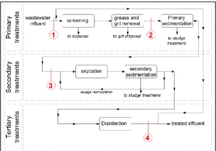
Figure 1.1 WWTP scheme for irrigation reuse ... 16
Figure 3.1 Description of the scientific method and the role of models [Dym and Ivey,1980] ... 27
Figure 3.2 Results of the first experiment on aerated batch sewage with enriched activated sludge by Arden and Lockett. (from (Hellenistic, 2007) ... 30
Figure 3.3 A timeline for AS modelling from (IWA Task Group on Good Modelling Practice, 2012) ... 31
Figure 3.4 Ludzack and Ettinger scheme ... 31
Figure 3.5 Modified Ludzack-Ettinger scheme ... 32
Figure 3.6 Number of publications on Activated Sludge models from 1985-2011 from Web of Science (IWA Task Group on Good Modelling Practice, 2012) ... 35
Figure 3.7 Schematic representation of the Peterson matrix ... 36
Figure 3.8 COD components in ASM1 ... 41
Figure 3.9 Nitrogen components in ASM1 ... 42
Figure 3.10 Cascade PI controllers implemented in aeration tank ... 49
Figure 3.11 BPM LIfecycle ... 50
Figure 4.1 Lemna minor in a FWS wetland ... 51
Figure 4.2 Processes involved in natural wastewater treatment with lagoons. Adapted from (Bragadin and Mancini, 2007) ... 52
Figure 4.3 One dimensional dispersion model. Adapted from (Butt, 2000) ... 53
Figure 4.4 Non ideal conditions PFR ... 56
Figure 4.5 Thirumurti chart adapted from (Mara, 2004) ... 58
Figure 5.1 A typical COD calibration curve ... 63
Figure 5.2 Ion selective electrode CRISON 9663C and a typical calibration curve ... 64
Figure 5.3 Chromatogram ... 64
Figure 5.4 M-TEC Agar ... 66
Figure 5.5 Petri plates after incubation. Red to magenta dots are E. coli colonies. ... 67
Figure 6.1 Multiprobe system YSI (from YSI 556 operation manual) ... 69
Figure 6.2 Beam used to fix the probes slot ... 69
Figure 6.3 Pyranometer PIRSC installed in Santerno WWTP area ... 70
Figure 6.4 WEST 2012 layout window ... 71
Figure 7.1 Bologna WWTP scheme with the numbers related to the measurement sections listed in Table 7.1 ... 77
Figure 7.2 Comparison between flow rate variations with BOD and COD (a) and with TSS and TKN (b) ... 79
Figure 7.3 Comparison between Input flow rate and COD (3a), TKN (3b), TSS (3c) in the sections 1,3,4 - Summer ... 80
Figure 7.4 Comparison between Input flow rate and COD (a), TKN (b), TSS (c) in the sections 1,3,4 - Winter ... 81
7
Figure 7.5 Ammonium in Input plant (section 1) and Input Biological (section 3) ... 82
Figure 7.6 Comparison between flow rate variations with TSS for rainy conditions ... 83
Figure 7.7. Comparison between flow rate variations with TSS for rainy conditions (6a) and dry conditions (6b) ... 84
Figure 8.1 Trebbo di Reno pilot plant scheme with flow rates. Q=inflow, QIR=internal recirculation, QR=sludge recirculation, QS=sludge surplus ... 85
Figure 8.2 Trebbo di Reno pilot plant ... 85
Figure 8.3 Trebbo di Reno pilot plant: secondary sedimentation ... 86
Figure 8.4 Treatment scheme of the Santerno WWTP in Imola (Bologna, Italy) ... 87
Figure 8.5 Santerno WWTP satellite view (from Google) ... 87
Figure 8.6 Santerno WWTP: Primary and secondary treatment scheme ... 88
Figure 8.7 Basin 1: view from the North (a) and South (b) sides ... 89
Figure 9.1 Santerno pilot plant : existing canal ... 90
Figure 9.2 Pilot plant: plan and sections. The sampling points are symbolized as black and white dots. Measures are in centimetres ... 92
Figure 9.3 Pilot plant: Baffle walls and final weir... 93
Figure 9.4 Pilot plant: from the outlet ... 94
Figure 10.1Trebbo pilot plant: COD Input ... 96
Figure 10.2 Trebbo pilot plant: Ammonium Nitrogen Input ... 96
Figure 10.3 Trebbo pilot plant: N-NH4+ input average concentration ... 97
Figure 10.4 Trebbo di Reno full scale WWTP: Influent flow rate ... 97
Figure 10.5 Basin 1 of natural finishing treatment with sections and measurement points in black and sampling points (a,b,c,d,i) ... 99
Figure 10.6 Basin 1 - section A-A' ... 100
Figure 10.7 Basin 1 – Section B-B’ ... 100
Figure 10.8 Basin 1 - section C-C' ... 100
Figure 10.9 Basin 1: sections with measured distances ... 101
Figure 10.10 Basin 1 - section D-D' ... 101
Figure 10.11 Solar Irradiance data 25/05/2016 ... 114
Figure 10.12 Solar Irradiance data 12/10/2016 ... 114
Figure 10.13 Solar Irradiance data 26/10/2016 ... 115
Figure 10.14 Solar Irradiance data 25/01/2017 ... 115
Figure 10.15 Solar Irradiance data 22/02/2017 ... 116
Figure 10.16 Santerno Pilot plant with sampling points ... 117
Figure 11.1 Case A: WEST 2012 layout ... 122
Figure 11.2 Case A: PI automatic control system. Blue arrow represents the variable measured in the aerobic tank and black arrows represent the adjusted variables ... 122
Figure 11.3 Case B: WEST 2012 layout ... 123
Figure 11.4 Case B: Automatic control system.Blue arrow represents the variable measured in the aerobic tank and black arrows represent the adjusted variables ... 124
Figure 11.5 Case B results: ammonium and nitrate output concentrations ... 124
8
Figure 11.7 Case C: Automatic control system.Blue arrow represents the variable measured in the
aerobic tank and black arrows represent the adjusted variables ... 126
Figure 11.8 Case C results: ammonium and nitrate output concentrations ... 126
Figure 11.9 Process layout in Bonita BPM ... 129
Figure 12.1 . Results for Ammonium Nitrogen (5a), Nitrate Nitrogen (5b) and Total Nitrogen (5c) in Basin 1 in four measurement campaigns ... 131
Figure 12.2 Basin 1: surface occupied by Lemna during the measurement campaigns ... 132
Figure 12.3 Basin 1: E.coli concentration measured in four sections ... 135
Figure 12.4 Santerno Pilot plant: Ammonium Nitrogen monitoring results ... 136
Figure 12.5 Santerno Pilot plant: E. coli monitoring results ... 137
Figure 12.6 Basin 1 scheme for E. coli model implementation ... 138
Figure 12.7 Basin 1: E. coli measured and modelled values 25/05/2016 ... 139
Figure 12.8 Basin 1: E. coli measured and modelled values 15/06/2016 ... 139
Figure 12.9 Basin 1: E. coli measured and modelled values 13/07/2016 ... 140
Figure 12.10 Basin 1: E. coli measured and modelled values 26/10/2016 ... 140
Figure 12.11Santerno pilot plant: E. coli measured and modelled values 12/10/2016 ... 141
Figure 12.12 Santerno pilot plant: E. coli measured and modelled values 25/01/2017 ... 142
Figure 12.13 Santerno pilot plant: E. coli measured and modelled values 22/02/2017 ... 142
Figure 13.1 Input physico-chemicals properties ... 144
Figure 13.2 Case LAS: Screen snapshot of the 9-box and 6-box worksheets with mass fluxes(mol/h) and removal efficiencies (%) through the primary settler (left), aeration tank (center) and secondary clarifier (right). ... 145
Figure 13.3 C12-LAS 2D structure from Pubchem database ... 146
Figure 13.4 LAS effluent modelling results under different KOC and KBIO conditions with secondary sedimentation (BOX9) ... 149
Figure 13.5 LAS effluent modelling results under different KOC and KBIO conditions without secondary sedimentation (BOX6) ... 149
Figure 13.6 Structural formula of BAC ... 150
Figure 13.7 BAC effluent in different KOC and KBIO conditions with (a) and without (b) secondary sedimentation compared with BAC effluent experimental (red line) ... 152
Figure 13.8 Experimental and calculated BAC removal efficiencies comparison ... 152
Figure 13.9 Nonylphenol effluent in different KOC and KBIO conditions with (a) and without (b) secondary sedimentation ... 154
Figure 13.10 Diclofenac 2D structure from Pubchem database ... 154
9
List of Tables
Table 2.1 Main international and European guidelines and regulations ... 22
Table 2.2 ISO 16075:2015: recommended parameters for each wastewater category ... 23
Table 2.3 WHO 2006 Guidelines: recommended parameters for restricted and unrestricted uses 24 Table 2.4 EPA 2012 Guidelines: recommended parameters for food and processed (or non-food) crops ... 24
Table 2.5 TN, COD and E. coli legal limits for irrigation reuse in some European countries ... 25
Table 2.6 Urban wastewater discharge thresholds (adapted from “Tabella 1” of Legislative Decree 152/2006) ... 25
Table 2.7 Urban wastewater discharge thresholds in case of discharging in sensitive areas (adapted from “Tabella 2” of Legislative Decree 152/2006) ... 26
Table 2.8 Main Italian standards for wastewater reuse (adapted from Ministry Decree DM 185/2003) ... 26
Table 3.1 Studies on AS process modeling and design from the 1950s and 1970s from (Angelakis and Joan, 2014) ... 33
Table 3.2 Grau Notation (adapted from (GRAU et al., 1983)) ... 37
Table 3.3 Monod-Herbert model : Peterson matrix representation from (Henze et al., 2000) ... 38
Table 3.4 Peterson matrix representation of ASM1 (Henze et al., 2000). ... 40
Table 3.5 State variables in ASM1 model ... 42
Table 3.6 Differential equations in ASM1 model ... 44
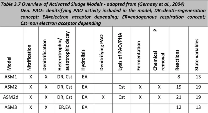
Table 3.7 Overview of Activated Sludge Models - adapted from (Gernaey et al., 2004) ... 45
Table 4.1 Convection and dispersion terms... 54
Table 4.2 Escherichia coli degradation model: parameters used ... 60
Table 5.1 Modified mTEC composition ... 65
Table 5.2 Phosphate buffered saline (PBS) composition ... 66
Table 5.3 Cultural characteristics after 22-24 hours at 44.5 +/- 0.2°C ... 67
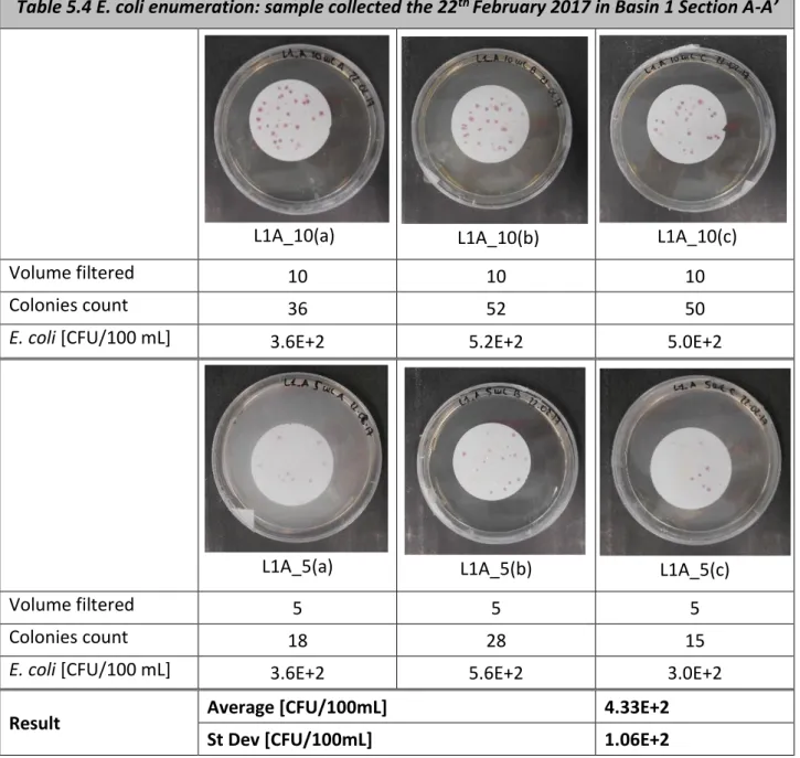
Table 5.4 E. coli enumeration: sample collected the 22th February 2017 in Basin 1 Section A-A’ .... 68
Table 7.1 List of the control parameters measured in each section of the Bologna WWTP ... 78
Table 8.1 Trebbo di Reno pilot plant tanks dimensions ... 86
Table 8.2 Santerno WWTP characteristics ... 88
Table 9.1 Santerno pilot plant design values ... 92
Table 10.1 Parameters of the model calibrated by (Pulcini, 2015) ... 98
Table 10.2 Basin 1 monitoring campaigns ... 99
Table 10.3 Basin 1: Total area and average water depth in each section ... 102
Table 10.4 Monitoring data 04-05-2016. Initial points: B and C’ ... 102
Table 10.5 Monitoring data 18-05-2016. Initial points: A, B, C’ and D ... 103
Table 10.6 Monitoring data 25-05-2016 Medium point in each section ... 105
Table 10.7 Monitoring data 15-06-2016. Initial points: A, B, C’ and D ... 106
10
Table 10.9 Basin 1 data: 25/05/2016 ... 111
Table 10.10 Basin 1 data: 15/06/2016 ... 112
Table 10.11 Basin 1 data: 13/07/2016 ... 112
Table 10.12 Basin 1 data: 26/10/2016 ... 113
Table 10.13 Basin 1 data: 30/11/2016 ... 113
Table 10.14 Basin 1 data: 22/02/2017 ... 113
Table 10.15 Santerno Pilot Plant monitoring campaigns ... 117
Table 10.16 Pilot plant data: 13/07/2016 ... 118
Table 10.17 Pilot plant data: 12/10/2016 ... 118
Table 10.18 Pilot plant data: 30/11/2016 ... 118
Table 10.19 Pilot plant data: 14/12/2016 ... 118
Table 10.20 Pilot plant data: 25/01/2017 ... 119
Table 10.21 Pilot plant data: 22/02/2017 ... 119
Table 10.22 Pilot plant monitoring data - 12/10/2016 ... 119
Table 10.23 Pilot plant monitoring data - 30/11/2016 ... 120
Table 10.24 Pilot plant monitoring data - 14/12/2016 ... 120
Table 10.25 Pilot plant monitoring data – 22/02/2017 ... 120
Table 11.1 Time-slot identification ... 121
Table 11.2 Case A: simulation results ... 123
Table 11.3 Case B: simulation results ... 125
Table 11.4 Case C: simulation results ... 127
Table 11.5 Recirculation rate used for the simulations ... 127
Table 11.6 Denitrification: simulation results ... 128
Table 12.1 Data from the Basin 1 – Santerno WWTP in Imola (Bologna, Italy) – Nitrogen concentration ... 131
Table 12.2 Basin 1: Temperature (T) and Dissolved Oxygen (DO) along the water column - 25/05/16 ... 133
Table 12.3 Basin 1: Temperature (T) and Dissolved Oxygen (DO) along the water column - 15/06/16 ... 134
Table 12.4 Basin 1: Temperature (T) and Dissolved Oxygen (DO) along the water column - 13/07/16 ... 134
Table 12.5 Basin 1: E. coli removal efficiency ... 135
Table 12.6 Santerno pilot plant: E. coli removal efficiency ... 137
Table 13.1 Chemicals selected to be modelled using Activity SimpleTreat ... 145
Table 13.2 Linear Alkylbenzene Sulfonate (LAS) physical-chemical input data ... 146
Table 13.3 Linear Alkylbenzene Sulfonate (LAS) Emission rate chemical ... 147
Table 13.4 LAS modelling results ... 148
Table 13.5 Benzalkonium chloride (BAC) physical-chemical input data ... 150
Table 13.6 BAC modelling results ... 151
Table 13.7 Nonylphenol (NP) physical-chemical input data ... 153
Table 13.8 Diclofenac physical-chemical input data ... 155
11
Table 13.10 Carbamazepine: simulation results ... 156 Table 13.11 Crops chosen and their cultivated surface in Emilia-Romagna Region in 2014- 2015 157 Table 13.12 Surface occupied by each crop in Emilia-Romagna Region in 2015 and their Irrigation
need ... 157 Table 13.13 Annual amount of selected chemical released in Emilia-Romagna ... 158
12
List of symbols
(-r) rate of reaction A reactor cross area C0 inlet concentration
D Axial dispersion coefficient D Axial dispersion coefficient f non dimensional concentration HRT Hydraulic Retention Time
Koc Organic carbon- water partition coefficient Kow octanol-water partition coefficient L reactor length
MAX maximum specific growth rate Pe Peclet number
pKaa acid dissociation constant of acids pKab acid dissociation constant of bases R reaction parameter
Re Reynolds number u axial velocity
13
List of abbreviations
APHA American Public Health Association
AS Activated Sludge
ASM Activated Sludge Model
BAC Benzalkoniium Chloride
BP Business Process
BPMN Business Process Management Notation
CFU Colony Forming Unit
DDD dose
E. coli Escherichia coli
EMR Emission Rate Chemical
ENEA Italian National agency for new technologies, Energy and sustainable economic development EPA United States Environmental Protection Agency
FAO Food and Agriculture Organization of the United Nations
FWS Free Water Surface
HERA Multiutility in Environmental, Water and Energy Services
IAWPRC International Association of Water Pollution Research and Control ICA Instrumentation Control Automation
LAB Linear Alkylbenzene
LAS Linear Alkylbenzene Sulfonate
MLE Modified Ludzack-Ettinger
NP Nonylphenols
NSAID Non-Steroidal anti-inflammatory drug ORP Oxidation Reduction Potential
ORP Oxidation Reduction Potential ORP Oxidation Reduction Potential PAOs phosphorus-accumulating organisms
PE Population Equivalent
PFR Plug Flow Reactor
PID Proportional Integer Differential
QAC Quaternary Ammonium Compounds
SBR Sequencing batch reactor
SSF Subsurface Flow System
St. Dev. Standard Deviation
TKN Total Kjeldahl Nitrogen
TN Total Nitrogen
TSS Total Suspended Solids
UCT University of Cape Town
UNEP United Nations Environment Programme
VSS Volatile Suspended Solids
14
Chapter 1. Introduction
1.1 Background and problem definition
In the last years, the role of wastewater treatment plants is even more relevant not only as final destination of the collected sewage but also as a center of the sustainable approach to the water cycle. Indeed, WWTPs management should play an important role in the frame of the circular economy recently supported by the European Commission with a specific action plan presented in 2015. This plan aims to support economical actors (business and consumers) as well as regional and national authorities in the transition through the circular economy. The circular economy aims at maintaining the value of products, materials and resources as long as possible, while reducing the waste production. Its final purpose consists in the generation of a more sustainable and competitive economy model for Europe. Specifically, the implementation of good practices in Wastewater Treatment plants (WWTPs) management allows not only to minimize the energy consumption maintaining the effluent concentrations under the law thresholds but also to reach different ends as wastewater reuse for industry or irrigation, energy production and raw material reservoir. The fast improvement of wastewater treatment control technologies supports this new sustainable management perspective. The use of ICA (Instrumentation Control and Automation) tools enables to regulate the processes minimizing energy requirements and consequently to reduce the managements costs (Olsson, 2015). Nowadays, automatic controls tools are commonly used in new plants and large-scale plants. However, many small-scale plants (< 50000 PE) are not provided with such tools. Indeed these small-scale plants need for accurate input signals and adequate measurement instruments that can prove to be expensive (Ingildsen and Olsson, 2001). Thus, a correct and efficient implementation of ICA tools requires a study of the correlation between the parameters measured and the processes. Moreover, the study of the signals from different sections of the plants and in different conditions allows to identify the main control sections and their characteristic parameters.
An incentive to increase the efficiency of WWTPs performances comes from the possibility to reuse the treated wastewater. Indeed, water scarcity has become more prominent in the last decades, increasing the need for new practices in terms of efficient water management. Reuse and valorisation of water from WWTPs can help solving the problem. Wastewater reuse history starts from the Minoan Civilization when water scarcity periods forced the use of very smart techniques. Several archaeological studies have revealed how Minoan sewer and stormwater drainage systems and their management for water reuse in palaces and cities were ahead of their time. In addition to the simple ‘grey water’ reuse, the combination of a stormwater drainage system with a wastewater system as well as the presence of little sedimentary tanks make Minoans the first civilization involved in the development of new techniques for wastewater reuse. All successive civilizations of the Mediterranean region, such as Ancient Greeks, applied these Minoan sanitary technologies
15
(Angelakis et al., 2005). Over the last years, the scarcity of water resources has been growing drastically, becoming a critical problem both in developing and industrialized countries. The agricultural sector, responsible for about 70% of annual global freshwater withdrawals (even up to 90% in some parts of Asia), is the biggest consumer of water (World Water Development Report 2016: Water and Jobs, 2016). In this context water reuse and more particularly wastewater reuse has a key role. The total amount of global reused water from wastewater treatment plants (WWTPs) in 2011 has been estimated to 7 Km3/year (Kirhensteine et al., 2016). Owing to the global increase of the agricultural field that requires almost 32% of irrigation reuse, the Global Water intelligence estimated an increase of reused water up to 26 Km3/year in 2030 (Kirhensteine et al., 2016). At European level, the volume of wastewater reuse was estimated in 2006 to 964 million m3/year (2.4 % of treated wastewater) (Kirhensteine et al., 2016), and its increase has been estimated to 1100 million m3/year for 2015 (BIO by Deloitte, 2015) and is expected to reach 3222 million m3/year in 2025 (Sanz and Bernd, 2014) . In 2006 water volume in Europe has been reused mostly by South-European countries (Raso, 2013) due to their higher water stress. However, this represents only a small part, between 5% to 12%, of the total treated wastewater, which indicates a great potential for those countries.
Finally, the WWTPs management must deal with new problems as the presence of emerging pollutants and their accumulation in the environment. Indeed, large amounts of xenobiotic compounds end in the plants and can be released in the environment because most of them are hardly or not biodegradable. Even if specific legal thresholds are not fixed yet, the problems related to these organic chemicals fate will become even more relevant in the WWTPs management especially in case of agricultural irrigation reuse (Polesel et al., 2015).
16
1.2 Aim of the thesis and methodology
The overall aim of this PhD thesis was to investigate the implementation of models in the most relevant sections of pilot and full scale plants and the possibility to reuse treated wastewater coming from the effluent flow rate of existing plants, or a part of it, for irrigation purpose. The study was referred to the treatment scheme showed in Figure 1.1. The scheme is divided in two parts in terms of management: “treatment” and “reclamation”. The first part is characterized by a common Activated Sludge (AS) scheme with Denitrification/Nitrification. The second part is made of a natural treatment basin for finishing with phytotreatment and lagoon. Moreover, the reclamation basin provides a natural disinfection and enable the water storage /release with respect to the irrigation request. The target ranges of the study were the small to medium WWTPs fed on mixed civil and industrialsewage.
The specific objectives of the thesis were:
1. to minimize the management costs of the “Treatment” using automatic controls. Different control solutions have been tested implementing the data acquired during a previous study on the pilot scale plant located in Trebbo di Reno (BO), in WEST 2012 software (DHI Software), based on ASM models. Moreover, a first approach on Business Process Management (BPM) applied to WWTPs has been tested;
2. to assess the parameters, control sections and measure instruments that influence the processes in unusual conditions. The monitoring data from Bologna real scale plant fed by urban combined sewage have been analyzed in flow variation conditions due to rain events. The effects of dry and rainy weather conditions on the process have been studied;
3. to test the effect of “Reclamation” phase on urban wastewater for irrigation reuse. This part has been developed in the frame of a partnership project with HERA, focused on the Santerno full scale WWTP located in Imola (Bologna, Italy). One-year measurement campaign has been carried on in the finishing lagoon section of the plant. Moreover, a pilot plant has been designed, built in the WWTP area and monitored in the same period. The pilot plant simulates the process occurring in the Basin 1 of the finishing phase of the plant, in different functioning conditions. It consists of a plug-flow reactor divided into two different reaction zones: FWS Phytotreatment-Lemna Minor and Aerobic Lagoon. Based on
17
the data acquired, the finishing effect on Nitrogen compounds and the natural disinfection effect on E. coli has been studied. The dispersed flow equation has been implemented to model the E. coli removal;
4. to predict the fate of organic chemicals, surfactants and pharmaceuticals, in conventional Activated Sludge plants and its load released in the soil during irrigation. This part has been developed during the research period at the Technical University of Denmark (DTU) – Section Environmental Chemistry, Department of Environmental Engineering under the supervision of Prof. Stefan Trapp as Short Term Scientific Mission (STSM) in the frame of the NEREUS COST Action ES1403 “New and emerging challenges and opportunities in wastewater reuse”. The residual chemical loads in the WWTP influent have been estimated starting from literature data in selected European plants. The Activity SimpleTreat model has been used to predict the fate of the selected chemicals in a generic sewage treatment plant. Finally, the loads of chemicals released by the most widely cultivated crops in Emilia-Romagna has been estimated.
18
1.3 Publications and conference contributions
Based on the research activity carried on during the PhD period, two scientific papers on international journals and eight contributions to international conferences were published, listed below in reverse chronological order.
Scientific papers published on international journals:
• Fiorentino Carmine; Mancini Maurizio; Luccarini Luca, Urban wastewater treatment plant provided with tertiary finishing lagoons: management and reclamation for irrigation reuse, «JOURNAL OF CHEMICAL TECHNOLOGY AND BIOTECHNOLOGY», 2016, 91, pp. 1615 - 1622 [scientific article]. (C. Fiorentino et al., 2016)
• Fiorentino Carmine; Mancini Maurizio; Luccarini Luca, Optimization of wastewater treatment plants monitoring in flow variation conditions due to rain events, «ENVIRONMENTAL ENGINEERING AND MANAGEMENT JOURNAL», 2016, 15, pp. 1981 - 1988 [scientific article] (Carmine Fiorentino et al., 2016).
Contribution to international conferences with proceeding and conference papers:
• Fiorentino, C., Mancini M., Avolio F. Anzalone F., Biomass recovery from the real scale Lemna FWS phytotreatment system implemented in Santerno WWTP , oral presentation in the Session “Water management within the circular economy. Resource recovery from the water cycle: market, value chains and new perspective for the water utilities and chemical industry” ECOMONDO 2016, 8-11 November 2016, Rimini, Italy [abstract and oral presentation]
• Mancini Maurizio; Fiorentino Carmine, Modelling and control of activated sludge wwtps under inflow variations due to a combined drainage system, in: Faculty of Civil and Industrial Engineering-SAPIENZA University of Rome, SIDISA 016 - Proceedings of X International Symposium on Sanitary and Environmental Engineering, Rome, DEI, 2016, pp. C07/2-1 - C07/2-13 (atti di: X International Symposium on Sanitary and Environmental Engineering-SIDISA 016, ROME, 19-23 June 2016) [Contribution to conference proceedings]
• Fiorentino Carmine; Mancini Maurizio; Ricci Roberto; Luccarini Luca, Modelling of control strategies and policies to manage urban wastewater treatment plants, in: Faculty of Civil and Industrial Engineering-SAPIENZA University of Rome, SIDISA 016 - Proceedings of X International Symposium on Sanitary and Environmental Engineering, Roma, DEI, 2016, 1, pp. E03/1.1 - E03/1.8 (atti di: X International Symposium on Sanitary and Environmental Engineering-SIDISA 016, ROME, 19-23 June 2016) [Contribution to conference proceedings] • Fiorentino Carmine; Mancini Maurizio, nitrogen removal effect of finishing lagoons on urban wastewater after secondary treatment, in: International Society for Environmental Biotechnology, Proceedings of the 10th International Society for Environmental Biotechnology Conference, 08034, Barcelona 2016, BarcelonaTech Jordi Girona, 1-3,, 2016, pp. 57 - 58 (conference proceedings: 10th International Society for Environmental Biotechnology Conference, Barcelona, 1-3 June 2016) [Abstract]
19
• Fiorentino, Carmine; Mancini, Maurizio; Luccarini, Luca, Optimization of Wastewater Treatment plants control in flow variation conditions due to rain events, in: GLOBAL WATER EXPO - Le acque di scarico: una risorsa da valorizzare, RIMINI, ECOMONDO, 2015, 1, pp. 1 - 1 (conference proceeding: ECOMONDO 2015 - The green technology EXPO, RIMINI, 3-6 november 2015) [Poster]
• Roberto Ricci; Luca Luccarini; Carmine Fiorentino; Maurizio Mancini, Modellazione di processo di un depuratore a fanghi attivi e sviluppo di strategie di controllo tramite Business Process, in: Atti della Italian DHI Conference 2015, Torino, DHI Italy, 2015, 1, pp. AU8.1 - AU8.40 (atti di: ITALIAN DHI CONFERENCE 2015, Torino, 14-15 october 2015) [Contribution to conference proceedings]
• Fiorentino, Carmine; Mancini, Maurizio; Luccarini, Luca, Optimization of wastewater treatment management and reclamation for irrigation reuse, in: E-proceedings - “6th European Bioremediation Conference" EBC VI 2015, Thessaloniki, Grafima Publications, 2015, 1, pp. 489 - 493 (atti di: 6th European Bioremediation Conference EBC VI 2015 - session 6c: Wastewater valorization, bioremediation, purification and reuse, Chania, Crete, Greece, June 29-July 2 2015) [Contribution to conference proceedings]
• M.L. Mancini; C. Fiorentino; L. Luccarini, Optimal set of control parameters for Wastewater Treatment Plants and optimization of instruments placement, in: Green Economy e sua implementazione nel Mediterraneo, Rimini, Maggioli Ed., 2014, 1, pp. 323 - 329 (atti di: ECOMONDO, Rimini, 5-8 sept 2014) [Contribution to conference proceedings]
20
Section 1
THEORETICAL FRAMEWORK
21
Chapter 2. Water and wastewater reuse
regulations
By defining correctly the water quality indicators, their specific reuse and threshold values, the development of guidelines and regulations for wastewater reuse plays a key role: first for the promotion of wastewater reuse and secondly for human health and environment protection. Historically, the State of California was the first in 1918 to promote water reuse with the adoption of the “Regulation Governing Use of Sewage for Irrigation Purposes”(California State Board of Health, 1918). For the first time, this Regulation set limits to the water reuse in agriculture and initiated the development of this technique in other states of the USA. Afterwards, international and national organizations focused on the wastewater safety through several regulations and guidelines for wastewater reuse.
At the European scale, a specific regulation for water reuse does not exist yet but several environmental directives are applicable in this field. Nevertheless, laws and standards for water reuse applications are written and implemented at member states and regional level. Regulations are thus highly heterogeneous, in particular in terms of intended uses, analytical parameters and threshold values (Sanz and Bernd, 2014). The main international guidelines for water and wastewater reuse for irrigation are listed in chronological order in Table 2.1.
22
Table 2.1 Main international and European guidelines and regulations
Year Organization Regulation Reference
1918 California State Regulation Governing Use of Sewage for Irrigation Purposes
(California State Board of Health, 1918)
1973 WHO Guidelines for Reuse of Water for
Irrigation (WHO, 1973)
1989 WHO and UNEP Guidelines (WHO, 1989)
1991 European Community
Urban Wastewater Directive
91/271/EEC (CEC, 1991)
1992 EPA Guidelines for water reuse (EPA, 1992)
1994 FAO Water quality for agriculture (Ayers and Westcot, 1994)
2003
Italy – Ministry of the Environmental and Protection of Land
Ministerial Decree (DM) (Ministry of Environment and Protection of Land, 2003)
2005 UNEP Guidelines for municipal water reuse
in the Mediterranean region (UNEP, 2005) 2006 WHO Guidelines for the safe use of
wastewater, excreta and greywater (WHO, 2006) 2007 Spain – Ministry of
Presidency Royal Decree (RD)
(Ministerio de Sanidad Servicios Sociales e Igualdad, 2007) 2011 Greece – Ministry of Environment, Energy and Climate Change
Common Ministerial Decision (CMD) (Government of Greece, 2011)
2011 UNEP
Development of performance indicators for the operation and maintance of wastewater treatment plants and wastewater reuse
(UNEP, 2011)
2012 EPA Guidelines for water reuse (USEPA, 2012)
2015 ISO
Guidelines for treated wastewater use
for irrigation projects (International Organization for Standardization, 2015)
23
Currently, the main international guidelines for wastewater reuse for irrigation are: ISO 16075:2015, WHO 2006 guidelines and FAO 2006 guidelines.
The ISO 16075:2015 classes the treated wastewater in five categories (A, B, C, D, E) depending on its treatment level and consequently its quality:
- Category A: very high quality treated water useable for agricultural irrigation of food crops consumed raw.
- Category B: high quality treated wastewater. The wastewater in this category can be used for urban irrigation and agricultural irrigation of processed food crops.
- Category C: medium quality treated wastewater. In this category the raw wastewater has been treated with physical and biological treatment and its use is agricultural irrigation of non-food crops.
- Category D: medium quality treated wastewater. As category C, the raw wastewater is treated with physical and biological processes and its use is for not potable applications of industrial and seeded crops.
- Category E: extensively treated wastewater. It is raw wastewater treated through natural processes and its use is for not potable applications of industrial and seeded crops.
Table 2.2 shows the parameters recommended for each category in terms of organic matter (BOD5), Turbidity or TSS and pathogens (Coliforms):
Table 2.2 ISO 16075:2015: recommended parameters for each wastewater category
Parameter Category A Category B Category C Category D Category E
BOD5 [mg/L] <10 <20 <35 <100 <35 Turbidity [NTU] 5 NR NR NR NR TSS [mg/L] <10 <25 <50 <140 NR Coliforms [CFU/100 mL] <100 thermo-tolerant coliforms <1000 thermo-tolerant coliforms <10000 thermo-tolerant coliforms NR NR Intestinal nematode [Egg./L] NR NR NR <5 <5 *NR = Not Reccomended
According to the WHO 2006 guidelines, two types of use are considered: unrestricted irrigation, when the treated wastewater will be used for not potable applications in settings where public access is not restricted, and restricted irrigation, treated wastewater used for non potable applications in public access areas.
24
Table 2.3 WHO 2006 Guidelines: recommended parameters for restricted and unrestricted uses
Parameter Unrestricted Restricted
TSS [mg/L] <10 <25
Coliforms [CFU/100 mL] E. coli <1000 E. coli <10000
Intestinal nematode [Egg/L] <1 <1
The EPA 2012 guidelines for water reuse give different parameters thresholds depending on the crops type: food crops, in case of irrigation of crops for human consumption consumed raw, and processed food crops or food crops not consumed by human.
Table 2.4 EPA 2012 Guidelines: recommended parameters for food and processed (or non-food) crops
Parameter For food crops For processes food crops
or non-food crops
BOD5 <=10 <=30
Turbidity <=2 Not recommended
TSS [mg/L] Not recommended <=30
Coliforms [CFU/100 mL] Fecal Coliforms Absence
Fecal Coliforms <=200 (Median)
Comparing the recommended parameters in the three cases it is possible to note that the parameter for organic matter is BOD5 and its thresholds are very strict in ISO 16075:2015 and EPA 2012 for food crops (<10 mg/L) while there is not any limit for organic matter in WHO 2006. TSS and turbidity thresholds are 5 NTU (ISO 16075:2015) and 2 NTU (EPA 2012) and again those are not considered in WHO 2006. The presence of high levels of turbidity can reduce the hydraulic conductivity of the soil, obstruct the irrigation facilities and, viruses and bacteria can migrate along with the solid particles. The recommended standards for pathogens are very stringent and can be achieved only through high cost technologies. This is a very real problem in developing countries.
An important change in some regulations (e.g. WHO 2006) is the use of the E. coli as bacterial indicators for water contamination instead of the traditional total and fecal coliform microbiological parameters because E. coli better represents the behaviour of pathogenic bacteria in water (Baudisova, 1997).
At the European level, several environmental directives exist and regulations are highly heterogeneous, in terms of intended uses, analytical parameters and threshold values (Sanz and Bernd, 2014).
25
E. coli is considered the pathogens parameter in many countries but the maximum thresholds are very different.
Table 2.5 shows the legal thresholds values for irrigation reuse in five European countries, referred to three main parameters: COD, TN and E. coli.
Table 2.5 TN, COD and E. coli legal limits for irrigation reuse in some European countries
Spain (RD1620/2007) Italy (DM185/2003) Greece (CMD 145116) France ( JORF 156/2014) Cyprus (Law 106/2002) COD [mg/L] - 100 - 60 70 TN [mgN/L] 10* 15 30 - 15 E. coli (CFU/100 mL] 0-10 4*** 10** 5-200 250-105 5-103
*Only for aquifer recharge and recreational uses
** It is the limit for 80% of the samples while 100 CFU/100mL is the maximum limit for all cases. The limit is higher using natural systems (phytodepuration or lagoons) becoming: 50 for 80% of the samples while 200 CFU/100mL is the maximum limit for all cases
*** The range is referred to different uses
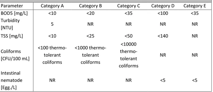
In this thesis, the Italian standards for wastewater discharge (Legislative decree 152/2006) and reuse (Ministry Decree 185/2003) are considered. The Legislative Decree 152/2016, also called “Code on the Environment”, implements two important European directives: the Water Framework Directive 2000/60/CE and the urban wastewater treatment 91/271/CE. The wastewater treatment rules are defined in the third part of the Legislative Decree (articles from 51 to 176) and the legal thresholds for urban wastewater discharge are in the annexes 5 in “Tabella 1”. “Tabella 2” indicates further thresholds for Total Phosphorus and Total Nitrogen when the effluent in discharged in sensitive areas. Table 2.6 and Table 2.7 below show the parameters and their legal limits as defined in “Tabella 1” and “Tabella 2“ of the Legislative Decree 152/2006.
Table 2.6 Urban wastewater discharge thresholds (adapted from “Tabella 1” of Legislative Decree 152/2006) Parameter WWTP capacity [PE] 2000 - 10000 > 10000 Concentration Reduction percentage Concentration Reduction percentage BOD5 [mg/L] <=25 70%-90% <=25 80% COD [mg/L] <=125 75% <=125 75% TSS [mg/L] <=35 90% <=35 90%
26
Table 2.7 Urban wastewater discharge thresholds in case of discharging in sensitive areas (adapted from “Tabella 2” of Legislative Decree 152/2006)
Parameter WWTP capacity [PE] 10000 - 100000 > 10000 Concentration Reduction percentage Concentration Reduction percentage Total Phosphorus [mgP/L] <=2 80% <=1 80% Total Nitrogen [mgN/L] <=15 70%-80% >=10 70%-80%
The Italian standards for wastewater reuse are fixed by the Ministry Decree (D.M. 185/2003) about “Technical measures for reuse of wastewater”.
Table 2.8 Main Italian standards for wastewater reuse (adapted from Ministry Decree DM 185/2003) limit Chemical Parameters BOD5 [mg/L] 20 COD [mg/L] 100 TP [mg/L] 2 TN [mg/L] 15 Ammonium [mg/L] 2 Chloride [mgCl/L] 250 Total surfactants [mg/L] 0.5 Microbiological parameters Escherichia coli 10 (80% of the samples) 100 (maximum limit in all the cases)
Using natural treatment systems (phytodepuration or wetponds)
50 (80% of the samples) 200 (maximum limit in all the cases)
Salmonella absent
The reference parameter for pathogen removal is E. coli and the output concentration limits are very strict, as shown in Table 2.8, making water reuse for irrigation hardly feasible from a process point of view.
27
Chapter 3. The Activated Sludge process and its
modeling
3.1 Mathematical modeling overview
Several definition and descriptions of mathematical modeling are available in literature. According to Hermann Schichl, a model “describes a typical human way of coping with the reality” (Kallrath, 2013) . He described the history of mathematical modeling since 2000 B.C. when the use of numbers can be recognized as the first way to model the reality.
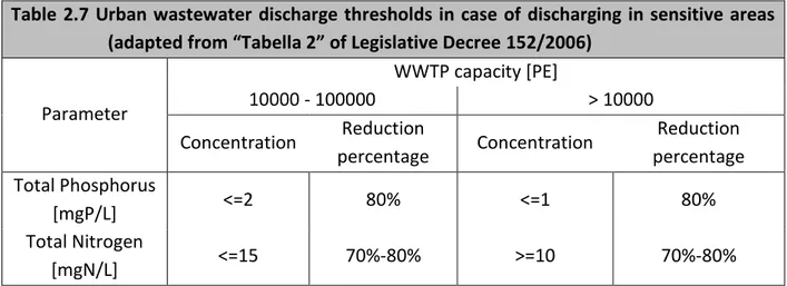
Dym and Ivey in “Principles of Mathematical Modeling” (Dym and Ivey, 1980), starting from the dictionary definition of model : “a miniature representation of something; a pattern of something to be made; an example for imitation or emulation; a description or analogy used to help visualize something (e.g., an atom) that cannot be directly observed; a system of postulates, data and inferences presented as a mathematical description of an entity or state of affairs” and mathematical model “a representation in mathematical terms of the behaviour of real devices and objects”, focused on the cognitive activity related to the modeling. This activity permits to describe the reality using, for instance, the mathematical language. They represented the scientific method as shown in Figure 3.1, where models play the key role to understand and predict real world phenomena
The real world The conceptual world
Observations
Phenomena Models
Predictions
Figure 3.1 Description of the scientific method and the role of models [Dym and Ivey,1980]
28
Therefore, models can be essentially used in two ways: to explain or predict a behaviour. Starting from these two approaches, we end with different applications of models. In Engineering, for instance, the prediction approach stands in the design phase while the explanation approach corresponds to the test phase. Moreover, models can be used to support the experimental method, when it is either too expensive, dangerous or time consuming (Jeppsson and Olsson, 1996).
Therefore, mathematical models have a long history but their implementation has been growing up significantly in the last decades thanks to the development of information technologies and the exponential growth of computational power.
In order to properly implement mathematical models, we have to define the work phases. Many approaches are proposed in literature to define these phases and two of them, related to studies on wastewater treatment plants modelling, are shown below. The first one is based on the guideline for simulation studies of wastewater treatment plants proposed by the HSGSim (Hochschulgruppe Simulation) research group. The HSG-guideline proposes the following seven phases:
1. Definition of objectives
2. Data collection and model selection 3. Data quality control
4. Evaluation of model structure and experimental design 5. Data collection for simulation study
6. Calibration/validation
7. Study and evaluation of success
The second approach is proposed by Jeppson (Jeppsson and Olsson, 1996) from a previous study by (Murthy et al., 1990) and considered five phases:
1. Functional process specification 2. Select modelling objectives 3. Select model type
4. Model construction methodology 5. Model validation
A comparison of both approaches reveals several common phases: definition of the objectives, selection of the model and the validation/calibration of the model. Moreover, the phase “Model construction methodology“ in the second approach is described as two phases in the first approach with a reference to data collection and evaluation.
The most important distinction in mathematical models for wastewater treatment processes is between steady-state and dynamic models. In steady-state conditions the model is not time dependent while in dynamic conditions time is a variable. The advantage of steady-state assumptions stands in its computational simplicity. Indeed, they are commonly used for model calibration. However, some processes require a more detailed and accurate description and consequently dynamic models are necessary despite of their computational cost.
29
A model is characterised by three mathematical properties: variables, constants and parameters. Their identification is the most important step to build or use a model.
Variables: these are the changing parts of the model and the most important are classified as input, output and state variables. The input variables are the initial information that the model need to run a simulation and to compute the output variables. In a dynamic model the state variables change during the calculations and represent the state of the process in a specific time. Output variables can also be state variables.
Constants: are all the components of the model that not change during the process (e.g. gravity). Parameters: are the mathematical quantities changeable for a process but constant for a specific implementation of them.
3.2 Activated Sludge process: historical perspective
The first studies and real implementations of artificial process for sewage treatment started in the second half of the 19th century and in the early 20th century. This period is marked by the end of the second industrial revolution and, as a consequence, by big economical and social changes that took place especially in Europe and United States. Increase of urban population and the change of conditions from a poor rural life to big cities, had negative effects on the environment and sanitary conditions. Frequent disease and epidemic killed thousands of people (eg., in 1832-33 cholera killed over 20,000 people in Britain).
Thanks to the development of microbiological research, we have started to correlate these health problems to water pollution and, consequently, to its management. Indeed, in the first half of the 19th century there was not any methods for sewage treatment and water supply technologies were very archaic. These problems were obviously more evident in the big cities of the most industrialised countries.
During the congress on “The Sewage of Towns” in 1866, the land treatment was established as the only acceptable sewage treatment system (Jenkins and Wanner, 2014). Consequently, this technology was adopted firstly in Britain and then in all European countries. Sewage was collected and spread on soil with good organic matter and removal efficiencies (eg. around 66% in Berlin). However, it was still not clear if the removal mechanisms were chemical or biological. Afterwards, an increase of removal efficiency in intermittent fed conditions has been evidenced. These conditions allowed the air flow inlet, contributing to the bacterial growth. Even if this bacterial process was not completely understood, it was clear that biological processes caused the organic matter and ammonia removal.
The main problem connected to this “natural” technology is big land requirement especially in densely populated cities. Then, new studies on more efficient technologies started during the later part of the 19th century. The first experiments on the biological processes were done at the Lawrence Experimental Station, Massachussetts in 1888 [Dumber 1899] where biological filters were aerated.
30
In 1912 Gilbert J. Fowler, researcher at University of Manchester, during a visit to United States (US), observed the experiments and started to study the effect of aeration on selected bacteria without recycling the settled solids.
Only in 1914 Edward Arden and William T. Lockett, two Fowler’s students, had the idea to collect the sludge from the settler and recycle it in the aerated batch. Using the settled sludge (called activated sludge by Arden and Lockett), they observed a reduction of total nitrification time and the increase of the purification efficiency (Orhon, 2014).The results were presented at the meeting of Society of Chemical Industry held on April 3rd 1914 at the Grand Hotel, Manchester, UK.
Pilot scale and then full-scale plants were implemented in the following years in Europe and US with encouraging results. The first activated sludge plant was constructed in 1920 in Sheffield, UK, and in 1926 in continental Europe (Essen-Rellinghausen, Germany).
The AS process had a great success as shown by the great amount of conference presentations patents and journal articles on this issue (around 606) from 1914 to 1921.
Figure 3.2 Results of the first experiment on aerated batch sewage with enriched activated sludge by Arden and Lockett. (from (Hellenistic, 2007)
31
3.3 The Ludzack-Ettiger scheme
In this work, the reference AS scheme is the Modified Ludzack-Ettinger (MLE), which is largely used to perform nitrogen removal.
The scheme was proposed for the first time in 1963 (Ludzack and Ettinger, 1963). It is based on two reactors in series partially separated: the anoxic and aerobic reactors (Figure 3.4). The partial separation between the anoxic and aerobic reactors enables the reduction of nitrate to nitrogen gas (denitrification process) in the anoxic reactor, also called pre-denitrification tank. The oxidation and nitrification processes occur in the aerobic reactor with the oxidation of ammonia to nitrite and then nitrate.
The scheme is also provided with the recirculation line from the secondary sedimentation to the aerobic reactor.
In 1973 Barnard proposed the MLE scheme in which the anoxic and aerobic tanks were completely separated and internal recirculation line was added. This internal recirculation allows to feed the pre-denitrification with the nitrate produced during the nitrification process.
Figure 3.4 Ludzack and Ettinger scheme
32
Therefore, the carbon and oxygen source for anoxic bacteria are respectively the influent wastewater and the internal recirculation while the recirculated activated sludge provides microorganisms (Figure 3.5).
3.4 Modeling the Activated Sludge process
During the first period after the discovery of the AS process (1920s-1950s), its application was widespread but very empirical. Different hypotheses were proposed to explain the removal mechanism and so a long time was also necessary to build a mathematical model.
In the 1940s, Jacques Monod, Nobel Prize in 1965, studied the bacterial growth using the Escherichia coli as biomass and lactic acid as substrate in his experiments.
In 1942 he proposed, in his doctorate thesis entitled “Recherche sur la croissance des cultures bactériennes”, the equation below that connects the bacterial growth rate (μ) and the substrate concentration (S) with a first order relationship:
𝜇 = 𝜇𝑀𝐴𝑋∙ 𝑆𝑆
𝐾𝑆+ 𝑆 (Eq. 3.1)
where:
- 𝜇𝑀𝐴𝑋 = maximum specific growth rate
- 𝑆𝑆 = concentration of the growth − limiting substrate - 𝐾𝑆 = half saturation constant
In particular, the half saturation constant corresponds to the substrate concentration when the growth rate is half of the maximum specific growth rate. Temperature and nutrients are not considered as limiting conditions in equation (Eq. 3.1).
Consequently, the biomass growth rate is: 𝑑𝑥 𝑑𝑡 = ( 𝜇𝑀𝐴𝑋∙ 𝑆𝑆 𝐾𝑆+ 𝑆 ) ∙ 𝑥 (Eq. 3.2) where: - 𝑥 = biomass concentration
33
Considering the coefficient of microbial growth (Y) as the ratio between biomass variation and substrate variation (dx/dS) the equation (Eq. 3.2) became:
𝑑𝑆 𝑑𝑡 = ( 𝜇𝑀𝐴𝑋 𝑌 ∙ 𝑆𝑆 𝐾𝑆+ 𝑆) ∙ 𝑥 (Eq. 3.3) where:
- 𝑌 = coefficient of microbial growth = dx dS The (Eq. 3.3) is the Michaelis-Menten equation.
After the Monod studies, several studies have been carried out on AS process modeling and design; the most relevant from 1954 to 1972 are listed in Table 3.1 below.
Table 3.1 Studies on AS process modeling and design from the 1950s and 1970s from (Angelakis and Joan, 2014)
1954 Eckenfelder and O’Connor Proposed a mathematical model for AS
1962 McKinney Proposed a completed mixing model
1968 Pearson Described the materials-balance model like approach to reactor analysis
1970 Lawrence and Carty proposed the material-balance model like approach to reactor analysis
1972 Metcalf and Eddy Incorporated the reactor theory approach
The most important improvement was around the 1950s when the soluble and particulate component of the organic matter of AS started to be considered.
In the 1970s the most advanced research centre on AS modeling was the University of Cape Town (UCT), South Africa, with the research group of prof. G.v.R Marais that developed the UCT model. At the beginning of the 1980s the need for model uniformization and guidelines induced the International Association of Water Pollution Research and Control (IAWPRC) to form a Task Group on mathematical Modeling for Design and Operation of Activated Sludge Processes.
The purposes were to review existing models for design and operation of biological wastewater treatment systems and create a common and simple platform that could be used for future development of AS models.
The final result was the Activates Sludge Model No. 1, called also IAWPRC model, ASM1 or IAWQ model, presented during the IAWPRC Specialised Seminar at KolleKolle, Denmark in 1985.
34
Afterwards, the ASM1 model was discussed by many researches in order to get a solid platform for the work and include details that could stand the test of time and was published in 1987 in its final form in the IAWPRC Scientific and Technical Report Series as STR No. 1.
The model was also a guideline for wastewater characterization and development of computer codes. Since its presentation, the ASM1 has been widely used for describing WWT biological processes all over the world and has been the core of numerous models with a number of supplementary details added for specific cases.
It was especially the matrix notation (Peterson, 1965), which was introduced together with ASM1 that facilitated the communication of complex models allowing to discuss the biokinetic aspects of the model with the common language.
The Task Group did not include the phosphorus removal because the modeling studies in this field were at the very beginning even if it was already used in full-scale treatment plants.
From the mid-1980s to the mid-1990s the biological phosphorus removal processes grew very popular and at the same time the understanding of the basic phenomena of the process was increasing. Thus in 1995 the Activated Sludge Model No.2 was published and it included nitrogen and phosphorus removal. In 1994, when the ASM2 was developed, the role of denitrification in relation of biological phosphorus removal was still unclear, so it was decided not to include that element.
Further developments in the research field lead to the understanding of denitrifying phosphorus-accumulating organisms (PAOs). Consequently, the Activated Sludge Model No.2 has been expanded in 1990 into the ASM2d model with the inclusion of denitrifying PAOs.
Afterwards, models gained in complexity and, in 1998, the Task Group decided to develop a new modeling platform, called the Activated Sludge Model No.3 (ASM3).
ASM3 introduced the concept of storage-mediated growth of heterotrophic organisms, assuming that all readily biodegradable substrate is firstly taken up and stored into an internal cell polymer component, which is then used for the biomass growth. Moreover, the model included the biological nitrogen removal model while the circular death-regeneration model was converted into growth-endogenous respiration model.
35
Figure 3.6 Number of publications on Activated Sludge models from 1985-2011 from Web of Science (IWA Task Group on Good Modelling Practice, 2012)
3.5 Format and notation: the Peterson matrix and Grau notation
The most important tasks in the development of a mathematical model are the identification of the processes involved and the selection of their respective kinetic and stoichiometric expressions. For these purposes, the Task Group decided that the best way to present models was the matrix format, based on the work of Peterson. Indeed, this representation offers the opportunity for overcoming the problem while conveying the maximum amount of information through a concise and intuitive representation of a large equation system. Furthermore, the Task Group recommended the use of a unique notation in order to have a common language: the Grau notation (GRAU et al., 1983).
The processes involved in the model are listed in the matrix raws and its components in the columns. The indexes j and i are assigned to processes and components respectively. The process rate equations or kinetic expressions are given in the last column. The kinetic parameters are listed in the last cell of the last column while the stochiometric parameters in the last cell of the first column. In the middle of the matrix there is the mass balance equation, which connects the processes involved and their kinetic and stoichiometric equations. Figure 3.7 below shows a schematic representation of the Peterson matrix.
36
Figure 3.7 Schematic representation of the Peterson matrix
The matrix contains all the information required to write the mass balance equations (ri) for each component (i) considering the kinetic expressions (ρj) of the processes (j) involved and the stoichometric parameters (νi). The generic equation:
𝑟𝑖 = ∑ 𝑟𝑖𝑗 𝑗
= ∑ 𝜈𝑖𝑗𝜌𝑗 𝑗
(Eq. 3.4)
enable to write the mass balance equations according to the basic equation: INPUT – OUTPUT + REACTION = ACCUMULATION
Conventionally the sign used in the matrix is positive for production and negative for consumption. Furthermore, the Task Group also decided to adopt the Grau nomenclature (Grau et al., 1983) in order to use a common language. Some quantities listed in the Grau notation and useful in AS modeling are shown below.
Soichiometric coefficients (ν
i)
Component (i)
P
roce
ss
(j
)
P
roce
ss
r
at
e
(ρ
j)
Mass balance
Components Unit
St
oi
chom
et
ri
c
par
am
et
er
s
K
ine
ti
c
pa
ra
m
et
er
s
37
Table 3.2 Grau Notation (adapted from (GRAU et al., 1983))
Symbol Quantity name or names Dimension
H Height or depth L L Length L δ Thickness L d Diameter L A Area L2 V Volume L3
X Particulate material concentration MiL-3
S Soluble material concentration MiL-3
C Total material concentration (particulate plus
+soluble) MiL
-3
rx Reaction rate per unit mass MiMx-1T-1
µ Specific biomass growth rate T-1 (from M
xMx-1T-1) µMAX Maximum specific biomass growth rate T-1 (from MxMx-1T-1)
bB Specific biomass loss rate T-1 (from M
xMx-1T-1)
Y Biomass yield coefficient MxMi-1
ν Stoichiometric coefficient MiMj-1
We briefly describe the use of the Peterson matrix and Grau notation, using the same example as the one given in the Task Group final report.
The aim of this model is to describe the heterotrophic bacteria growth and decay in aerobic conditions. Each unit of substrate generates Y units of biomass using 1-Y units of oxygen.
The first step is the definition of the processes and components involved. Here, two processes are involved: aerobic growth of biomass (j=1) and its loss by decay (j=2). The components (or variables) are: heterotrophic biomass (XB), soluble substrate (SS) and oxygen (So). Note that according to the Grau notation X and S represent respectively the particulate and the soluble material concentrations.
The kinetic expressions came from the Monod-Herbert model, where the biomass aerobic growth is calculated with the Monod equation (Eq. 3.1) while the biomass decay is calculated with the Herbert equation:
𝑑𝑥 𝑑𝑡 = 𝑏𝑥
38
Table 3.3 Monod-Herbert model : Peterson matrix representation from (Henze et al., 2000) Therefore, the mass balance equation system can be easily written using the ri expression in Table 3.3: { 𝑟𝑋𝐵 = 𝜇̂𝑆𝑆 𝐾𝑆+ 𝑆𝑆𝑋𝐵− 𝑏𝑋𝐵 𝑟𝑆𝑆 = −1 𝑌 𝜇̂𝑆𝑆 𝐾𝑆+ 𝑆𝑆𝑋𝐵 𝑟𝑆0 = −1 − 𝑌 𝑌 𝜇̂𝑆𝑆 𝐾𝑆+ 𝑆𝑆𝑋𝐵− 𝑏𝑋𝐵 (Eq. 3.6)
Moreover, the matrix annotation enables to check the continuity condition: moving along the rows, as indicated by the arrow in Table 3.3, the sum of the stoichiometric coefficients must be zero.
39
3.6 Activated Sludge Model n°1 (ASM1)
Presented in 1985 for the first time, the ASM1 model has been widely used for describing WWT biological processes and became a basis for further models development.
The purpose of this model was to describe the carbon and nitrogen removal through the activated sludge process with biological oxidation, nitrification and denitrification.
The biomass involved in those processes is:
- Heterotrophic bacteria, they use organic carbon for growth and are responsible of the denitrification process in the anoxic tank and the organic substrate degradation in aeration tank. The most common denitrifying bacteria are Bacillus denitrificans, Micrococcus denitrificans, Pseudomonas stutzeri and Achrornobacter. In anaerobic conditions, these organisms use nitrate or nitrite as terminal electron acceptors and oxidizing organic matter for energy. The result is the reduction of nitrate to nitrogen gas.
- Autotrophic bacteria, they use inorganic carbon for growth and are responsible of nitrification in the aerobic tank. The most common genera involved in nitrification are Nitrosomonas and Nitrobacter. Nitrosomonas can only oxidize ammonia nitrogen to nitrite nitrogen while Nitrobacter oxydize nitrite nitrogen to nitrate nitrogen.
The ASM1 model is based on three hypotheses:
- Bisubstrate: the substrate is divided in two fractions of COD readily and slowly biodegradable.
- Michaelis-Menten Kinetic (see (Eq. 3.3).
- Growth-decay: the result of the biomass decay is only non-biodegradable matter representing the inert residue.
40
![Figure 3.1 Description of the scientific method and the role of models [Dym and Ivey,1980]](https://thumb-eu.123doks.com/thumbv2/123dokorg/8128835.125759/27.892.254.636.660.1003/figure-description-scientific-method-role-models-dym-ivey.webp)