Turbulent Diffusion of the Geomagnetic Field and Dynamo Theories

Alma Mater Studiorum

Alma Mater Studiorum –

– Università di Bologna

Università di Bologna

DOTTORATO DI RICERCA IN

Geofisica

Ciclo XXVII

Settore Concorsuale di afferenza: 04/A4

Settore Scientifico disciplinare:GEO/10

TITOLO TESI

Turbulent Diffusion of the Geomagnetic Field and Dynamo

Theories

Presentata da:

Enrico Filippi

Coordinatore Dottorato

Relatore

Prof. Nadia Pinardi

Dott. Angelo De Santis

Correlatore

Prof. Maurizio Bonafede

Contents

List of Figures 4

List of Tables 5

Abstract 7

Introduction 9

1 The Earth’s Magnetic Field: Dynamo Theories 11 1.1 Introduction . . . 11 1.2 Magnetic Induction Equation . . . 12 1.2.1 Toroidal and poloidal vectors. Free decay modes for a sphere . 14 1.3 Internal and external sources . . . 16 1.4 Spatial and temporal spectra of the Geomagnetic Field . . . 17 2 Random forcing in isotropic turbulence and Magnetohydrodynamics 19 2.1 A first approach to homogeneous isotropic turbulence . . . 19 2.2 Random Forcing and Turbulence in Magnetohydridynamics . . . 20 3 Turbulent diffusive regime of the geomagnetic field during the last

millen-nia 21

3.1 Magnetic induction equation and diffusion . . . 21 3.2 Global models analysis . . . 24 3.2.1 Paleomagnetic and IGRF models . . . 24 3.2.2 Time scales, turbulent diffusivity and apparent core conductivity . . 26 4 Outer Core Dynamics and rapid intensity changes 41 4.1 Introduction . . . 41 4.2 Methodology . . . 42

5 Discussion and Conclusions 47

A Calculation of the mean electromotive force 51

List of Figures

1.1 Reference frame for the magnetic field. I is the inclination or latitude. D is the declination or longitude (Figure by Parker, 2005). . . 11 1.2 Schematic representation of the different sources responsible for the Earth’s magnetic field. 12

1.3 Temperature vs depth (Figure by http://www.nhn.ou.edu/~jeffery/astro/astlec/lec011/earth_004_temperature.png).

13

1.4 Energy density vs n. . . 17

3.1 ln (g10)2 vs t. The red parts of this graphic represent temporal in-tervals longer than 100 years when ln (g10)2decreased approximately linearly with time; so we have decided to estimate τi by the data of these intervals. The g10coefficients were synthesized by CALS7k model except for the last red interval when the coefficients were synthesized by IGRF model. . . 28 3.2 Temporal trend of the geomagnetic field power on the Earth’s Surface

and on the Core Mantle Boundary (CMB)(Figure by Korte and Con-stable, 2005). . . 29 3.3 ln (g10)2 vs t. The red parts of this graphic represent temporal

in-tervals longer than 100 years when ln (g10)2decreased approximately linearly with time; so we have decided to estimate τi by the data of these intervals. The g10coefficients were synthesized by CALS10k model. 30 3.4 ln (g10)2 vs t. The red parts of this graphic represent temporal

in-tervals longer than 100 years when ln (g10)2decreased approximately linearly with time; so we have decided to estimate τi by the data of these intervals. The g10coefficients were synthesized by CALS3k model. 31 3.5 Histogram about the 10000 decay times got by a bootstrap method in

the age between 11200 B.C and 11080 B.C. . . 33 3.6 Histogram about the 10000 apparent conductivities got by a bootstrap

method in the age between 11200 B.C and 11080 B.C. . . 34 3.7 Histogram about the 10000 decay times got by a bootstrap method in

the age between 6460 B.C and 6320 B.C. . . 35 3.8 Histogram about the 10000 apparent conductivities got by a bootstrap

method in the age between 6460 B.C and 6320 B.C. . . 36 3.9 Histogram about the 10000 decay times got by a bootstrap method in

the age between 1750 A.D. and 1875 A.D. . . 37 3.10 Histogram about the 10000 apparent conductivities got by a bootstrap

3.11 Analysis of several Geomagnetic Axial dipoles vs t ; blue lines: g01by sha.dif.14k; pink lines: strong decays of g01by sha.dif.14k; green lines: g01by cals10k; red lines: strong decays of g01by cals10k; yellow lines: g01by pfm9k.1; black lines: strong decays of g01by pfm9k.1; purple line: g01by IGRF12 . (Figure by Filippi et al., 2015) . . . 39 4.1 Maximum temporal variation of g01 in the ages between 1980 A.D.

and 2015 A.D. (these coefficients are by IGRF12 model (Thebault et al., 2015)) . . . 44 4.2 Maximum temporal variation of g01 in the ages between 1980 A.D.

and 1990 A.D. (these coefficients are by CALS10k model (Korte et al., 2011)) . . . 45 4.3 Maximum temporal variation of g01 in the ages between 1980 A.D.

and 1990 A.D. (these coefficients are by CALS3k model (For reference about this modelKorte and Constable, 2003 and Korte et al., 2009)) . 46

List of Tables

1.1 Curie temperatures of some materials in the Earth (For references see e.g. Blaney, 2007, Heller, 1967, Kolel-Veetil and Keller, 2010, Pan et al., 2000) . . . 12 3.1 Relaxation times and apparent electrical conductivities estimated by

CALS7k and IGRF data. Relaxation times (and associated errors) and apparent conductivities (and associated errors) are approximated at the closest hundred and thousand, respectively. . . 29 3.2 Relaxation times and apparent electrical conductivities estimated by

CALS10k data. Relaxation times (and associated errors) and apparent conductivities (and associated errors) are approximated at the closest hundred and thousand, respectively. . . 30 3.3 Relaxation times and apparent electrical conductivities estimated by

CALS3k data. Relaxation times (and associated errors) and apparent conductivities (and associated errors) are approximated at the closest hundred and thousand, respectively. . . 31 3.4 Relaxation times and apparent electrical conductivities estimated by

SHA.DIF.14k data. Relaxation times (and associated errors) and ap-parent conductivities (and associated errors) are approximated at the closest hundred and thousand, respectively. . . 32

Abstract

The thesis deals with the Dynamo Theories of the Earth’s Magnetic Field and mainly deepens the turbulence phenomena in the fluid Earth’s core. Indeed, we think that these phenomena are very important to understand the recent decay of the geomagnetic field. The thesis concerns also the dynamics of the outer core and some very rapid changes of the geomagnetic field observed in the Earth’s surface and some aspects regarding the (likely) isotropic turbulence in the Magnetohydrodynamics. These topics are related to the Dynamo Theories and could be useful to investigate the geomagnetic field trends.

Introduction

The thesis deals with the Dynamo Theories of the Earth’s Magnetic Field and mainly deepens the turbulence phenomena in the fluid Earth’s core. Indeed, we think that these phenomena are very important to understand the recent decay of the geomagnetic field. The thesis concerns also the dynamics of the outer core and some very rapid changes of the geomagnetic field trend observed in the Earth’s surface and some aspects regarding the (likely) isotropic turbulence in the Magnetohydrodynamics. These topics are related to the Dynamo Theories and could be useful to investigate the geomagnetic trends.

In Chapter 1 we introduce the Magnetic Field of the Earth and the Dynamo Theo-ries. More specifically, we briefly describe the main sources of the Magnetic Field of the Earth, we recall Maxwell equations in the Earth core and we derive the Magnetic Induction Equation by making some suitable geophysical approximations. We Finally, in a particular case, we discuss some properties and features of the geomagnetic field as the decay times.

The aim of Chapter 2 is to extend a methodology about Random Forcing in isotropic turbulence in order to understand better the dynamics of the fluid Earth’s Core. We explain some previous studies and computational methods aimed to study some tur-bulence problems. These methods use the "Random forcing" techniques in order to investigate on the isotropic turbulence of Navier-Stokes equation. The purpose is to adapt these methods to treat isotropic turbulence in Magnetohydrodynamics by mod-ifying in a suitable way some codes used by M. Maxey(see e.g.Ruetsch and Maxey, 1991).

In Chapter 3 we deal with some turbulent dynamo theory problems. In other words, we discuss how some small scale phenomena affect the trend of the geomagnetic field. We study the temporal behaviour of the geomagnetic field in the last few millennia in the context of turbulent dynamo theory. We consider several global geomagnetic models concerning up to 14000 years. In particular we analyze the recent trend of the dipolar geomagnetic field, in order to find some evidences for a turbulent diffusivity. This work contributes, in an original way, to improve the knowledge of the geodynamo turbulent regime and helps to understand how much of this regime can be observed in the recent geomagnetic field. Moreover our approach uses a new method and our study concerns a temporal interval greater than the interval considered by previous works.

In Chapter 4 we consider some large scale dynamo theory problems. We use an optimization method in order to estimate the rapid changes of the dipolar geomagnetic field. This method was firstly developped by P.W. Livermore, A. Fournier and Yves Gallet ( Livermore et al., 2014) in order to evaluate the maximum of the intensity variations and to search the links between the outer core dynamics and rapid changes of the geomagnetic field. Here we modify this method in a suitable way to our setting and we present the related results. This extension is new, flexible and it could have

Chapter 1

The Earth’s Magnetic Field:

Dynamo Theories

1.1 Introduction

The geomagnetic field is an important property of our planet and it is shared with other planets in the solar system and with the Sun itself. We can use the magnetic compass because the magnetic field is a vector quantity, so it has a magnitude and a direction; this feature requires to introduce a suitable reference frame to describe properly the geomagnetic field as the following:

Gilbert’s earlier speculation. He was also responsible for beginning the measurement of the geomagnetic

field at globally distributed observatories, some of which are still running today.

Figure 1.1

The magnetic field is a vector quantity, possessing both magnitude and direction; at any point on Earth

a free compass needle will point along the local direction of the field. Although we conventionally think

of compass needles as pointing north, it is the horizontal component of the magnetic field that is directed

approximately in the direction of the North Geographic Pole. The difference in azimuth between magnetic

north and true or geographic north is known as declination (positive eastward). The field also has a vertical

contribution; the angle between the horizontal and the magnetic field direction is known as the inclination

and is by convention positive downward (see Figure 1.1). Three parameters are required to describe the

magnetic field at any point on the surface of the Earth, and the conventional choices vary according to

subfields of geomagnetism and paleomagnetism . Traditionally, the vector B at Earth’s surface is referred to

a right-handed coordinate system: north-east-down for x-y-z. But often instead of using the components in

this system, three numbers used are: intensity, B =

_{|B|, declination, D, and inclination, I as shown in the}

sketch or D, H and Z; H, or equivalently B

h

, is the projection of the field vector onto the horizontal plane

and Z, or equivalently B

z

, is the projection onto the vertical axis. D is measured clockwise from North

and ranges from 0

_{→ 360}

◦

(sometimes

₋₁₈₀

◦

_{→ 180}

◦

). I is measured positive down from the horizontal

and ranges from

_{−90 → + 90}

◦

(because field lines can also point out of the Earth, indeed it is only in the

northern hemisphere that they are predominantly downward). From the diagram we have

H = BcosI;

B

z

= BsinI.

(1)

2

Figure 1.1: Reference frame for the magnetic field. I is the inclination or latitude. D is the declination or longitude (Figure by Parker, 2005).

If B is the magnitude of the geomagnetic field B, D is the declination and I is the inclination, by the Figure 1.1 we can easily deduce that

Bx= B cos I cos D By = B cos I sin D

Bz= B sin I

1.2 Magnetic Induction Equation

In this section we deduce and analyze the Magnetic Induction Equation in a similar way as it is done in Gubbins and Roberts, (1987).

Figure 1.2:Schematic representation of the different sources responsible for the Earth’s magnetic field.

In the Earth the main sources of the magnetic field are located in the outer Core (see Fig. 1.2), namely the fluid region inside the Earth between 3000 and 5000 km depth. This region is constituted mainly of iron and its compounds although there are also other material like Mg, Ni, O, S, Si; however the concentration of these materials is much less than that of iron and its compounds.

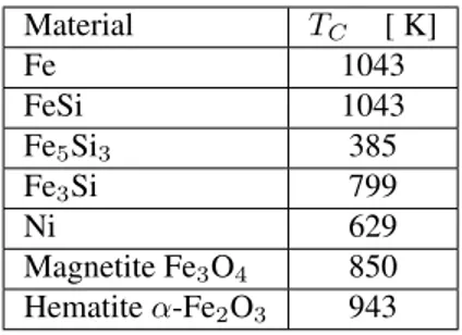
Material TC [ K] Fe 1043 FeSi 1043 Fe5Si3 385 Fe3Si 799 Ni 629 Magnetite Fe3O4 850 Hematite α-Fe2O3 943

Table 1.1: Curie temperatures of some materials in the Earth (For references see e.g. Blaney, 2007, Heller, 1967, Kolel-Veetil and Keller, 2010, Pan et al., 2000)

1.2 Magnetic Induction Equation 13

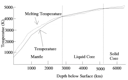
Figure 1.3:Temperature vs depth (Figure by http://www.nhn.ou.edu/~jeffery/astro/astlec/lec011/earth_004_temperature.png).

See e.g. Ganguly, (2009) and Dziewonski and Anderson, (1981) for references on the Earth Interior temperature gradient and on the Outer Core.

In order to deduce the most important equations in the Dynamo Theory, firstly we recall the Maxwell Equations:

           ∇ · D = ρe ∇ · B = 0 ∇ × E = −∂B ∂t ∇ × H = J +∂D ∂t (1.1)

Where D = εE, B = µH, ρe is the electrical density and J is defined by the well-known Ohm’s law, namely

J = σE + σ(v × B) (1.2)

Here D is the electric displacement, E and B are the electric and magnetic field, H is the magnetizing force and J is the electric current density vector. If we look at Fig. 1.4 and Table 1.1, we can state that the temperature in the core is much higher than the typical Curie temperatures of the materials compounding the core itself; this fact allow us to say that, in the outer core, the magnetic permeability is almost equal to the vacuum magnetic permeability and also the dielectric permeability is almost equal to the vacuum dielectric permeability, namely

B = µH � µ0H (1.3)

and

D = εE � ε0E (1.4)

If we introduce some suitable spatial and temporal scale L and T , we can define the orders of magnitude of the L.H.S. and of ∇ × E and of ∂B

∂t in this way:

and _� � � �∂B∂t � � � � ≈ BT (1.6)

where B and E are the typical mean values of the magnetic and electric field. The III Maxwell’s equation and a comparison between (1.5) and (1.6) lead to:

E B ≈

L

T (1.7)

So, bearing in mind the (1.3), (1.4) and the (1.7) we can state that � �∂D ∂t � � |∇ × H| ≈ ε0µ0(L/T ) 2 _(1.8)

But from electromagnetic theory ε0µ0 = 1/c2, where c is the light speed; the typical geomagnetic length-scales and time-scales allow us to say that the ratio (L/T ) is � c (for references see e.g. Backus et al., 1996 and Parker, 2005); in other words in Geo-magnetism we can neglect the displacement current.

∇ × H ≈ J (1.9)

The expression written above is called Magnetohydrodynamic approximation. By tak-ing the curl of the IV Maxwell’s equation and beartak-ing in mind the (1.2), (1.3) and the (1.9) we obtain: ∂B ∂t = 1 σµ0∇ 2_{B + ∇ × (v × B) (1.10)}

The equation (1.10) is called Magnetic Induction Equation and it is the most im-portant equation in the Dynamo Theory and in Magnetohydrodynamics.

1.2.1 Toroidal and poloidal vectors. Free decay modes for a sphere

B = ∇ × ψTr + ∇ × (∇ × ψPr) = BT+ BP (1.11) Now, it is convenient to use the spherical coordinates (r, θ, φ), where r is the radius, θ is colatitude and φ is the latitude.

BT = � 0, 1 sin θ ∂ψT ∂φ ,− ∂ψT ∂θ � (1.12) BP= �ˆ_l2_ψ P r , 1 r ∂2_(rψ P) ∂θ∂r , 1 r sin θ ∂2_(rψ P) ∂φ∂r � (1.13) where ˆl2_{is the angular-momentum operator in quantum mechanics, namely}

ˆl2 ≡ −� 1_{sin θ∂θ}∂ � sin θ ∂ ∂θ � + 1 sin2_θ ∂2 ∂φ2 �

Note that the toroidal field BTcannot be measured on the Earth’s Surface, because its radial component vanishes.

1.2 Magnetic Induction Equation 15 Now, if we consider the simple case where v = 0, the (1.10) is equal to the well-known diffusion equation

∂B ∂t = η∇

2_{B (1.14)}

with η = 1

µ0σ; it is very easy to prove that any solution of the (1.14) can be written like the (1.11) where ψT and ψP are solutions of the following equations:

     ∂ψT ∂t = η∇ 2_ψ T ∂ψP ∂t = η∇2ψP (1.15) The (1.15) can be solved by some standard techniques described e.g. in Gubbins and Roberts, (1987). After developping these techniques we can state that two solutions of the (1.15) are: ψT(r, θ, φ, t) = ∞ � l=1 l � m=0 tml (r)ylm(θ, φ) � ν e−t/τνl (1.16) ψP(r, θ, φ, t) = ∞ � l=1 l � m=0 pml (r)ylm(θ, φ) � ν e−t/τνl (1.17) where ylm(θ, φ) =� (2l + 1)(l − |m|)! 4π(l + |m|)! �1/2 1 2l_l!sin m_θdl+|m|(cos2θ− 1)l d(cos θ)l+|m| e imφ tm l = hlmjl �_k Tr RC � pml = qlmjl �_k Pr RC � and τνl= R2 C η(kνl)2 (1.18)

where hlm and qlmare constants, jlare the Bessel functions of half-integer order, RCis the radius of the outer core, kT and kPare the solutions of the equations:

jl(kT) = 0 (1.19)

jl−1(kP) = 0 (1.20)

τνlare the decay times and each kνlis the ν-th solution of the equations (1.19), (1.20) Equations (1.18)-(1.20) can be easily derived according to Gubbins and Roberts, (1987), by using the following property of the Bessel functions (see e.g. Abramowitz and Stegun, 1970)

j�l(x) + (l + 1) jl(x)

x = jl−1(x) (1.21)

[ˆn · B] = 0 su r = RN (1.22)

[ˆn × B] = 0 su r = RN (1.23)

[ˆn × E] = 0 su r = RN (1.24)

[ˆn · J] = 0 su r = RN (1.25)

[ˆn · E] �= 0 su r = RN (1.26)

where [ ] denotes the jump across the Outer Core Surface.

1.3 Internal and external sources

We said in Section 1.2 that the main sources of the Geomagnetic Field are in the Outer Core. However, there are some relevant geomagnetic field sources also in the iono-sphere, the region of the upper atmosphere where the ionization is much greater than in the low atmosphere. Indeed, this great ionization creates several electric currents (see Fig. 1.2). In other words, the main sources of the geomagnetic field are in the Outer Core (internal sources) and in the Ionosphere (external sources). From (1.9), we can formalize this fact in the following way:

   ∇ × B(r, θ, φ) = 0 if RCM B≤ r < Rion ∇ × B(r, θ, φ) = µ0JC if RICB ≤ r < RCM B ∇ × B(r, θ, φ) = µ0Jion if r≥ Rion (1.27) where RCM Bis the radius of the Outer Core, RICBis the radius of the Inner Core, Rion is the radius of the Ionosphere (by CMB we mean the Core Mantle Boundary, and by ICB the Inner Core Boundary). So, the B can be represented as a conservative field, if RCM B ≤ r < Rion. This fact together with the II Maxwell’s equation, allow us to state that if RCM B≤ r < Rion:

   B = −∇V ∇2_{V = 0} V = Vint+ Vext (1.28) where: Vint= a Ni � n=1 n � m=0 � a r �n+1

(gnmcos(mφ) + hnmsin(mφ))Pnm(cos θ) (1.29) and Vext= a Ni � n=1 n � m=0 � r a �n

1.4 Spatial and temporal spectra of the Geomagnetic Field 17

1.4 Spatial and temporal spectra of the Geomagnetic

Field

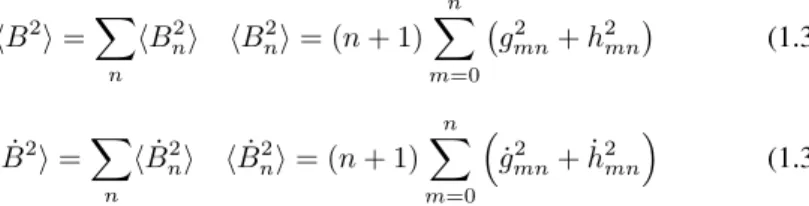
According to the contribution of De Santis et al., (2003), we can introduce the spatial and temporal spectra of the Geomagnetic Field. The spatial spectrum of the Geomag-netic Field and of its first temporal derivative ˙B are:

�B2� =� n �Bn2� �Bn2� = (n + 1) n � m=0 � gmn2 + h2mn � (1.31) � ˙B2 � =� n � ˙B2 n� � ˙Bn2� = (n + 1) n � m=0 � ˙g2 mn+ ˙h2mn � (1.32) where gmnand hmnare the coefficients defined at the end of the previous section and

˙gmnand ˙hmnare their time derivatives. It is possible to express:

�B2n� = keαn (1.33)

� ˙B2n� = k�eα

�_n

(1.34) where k, k�_{, α and α}� _{are suitable parameters. It is important to note that by means of} the geomagnetic spatial spectrum we can distinguish core from crustal fields (see e.g. De Santis et al., 2016 ). ! ! ! ! "! ! #$%&'!()'&! ('$*%!

By the (1.33) and (1.34) we can define the temporal spectrum in the following way: �B2 n� ∝ (en)α= ω−γn (1.35) where ωn = � k� ke −(α−α�_)n/2 and γ = 2α α_{− α}�.

Chapter 2

Random forcing in isotropic

turbulence and

Magnetohydrodynamics

In this chapter we describe a methodology about Random Forcing in isotropic turbu-lence in order to highlight the dynamics of the fluid Earth’s Core. We explain some previous studies and computational methods aimed to study some turbulence prob-lems. These methods use the "Random forcing" techniques in order to investigate on the isotropic turbulence of Navier-Stokes equation. Our aim is to discuss how much is important the the turbulence in Magnetohydrodynamics and how can be observed in the trend of the Geomagnetic Field.

2.1 A first approach to homogeneous isotropic

turbu-lence

There are several works that used the Random Forcing methods to study the rotational form of the Navier-Stokes equation, namely:

∂v ∂t + ω × v = −∇ �_p ρ+ 1 2|v|2 � + ν∇2_{v (2.1)}

Firstly, we briefly explain a method to study a problem in homogeneous isotropic tur-bulence developped in Ruetsch and Maxey, (1991). This method for simplicity’ s sake uses a simplified geometry. It considers a cube of side L = 2π, that is discretized into N3_{grid points, with periodic boundary conditions in all three directions. The grid} points in physical space are defined as

(xi, yj, zk) = � L Ni, L Nj, L Nk � (2.2) where i, j, k = 1, 2, ..., N. The grid points in Fourier space, or wave-number compo-nents, are of the form:

where ni = 0, 1, 2, ..., N/2 for i = 1, 2, 3. Data specified at the physical grid points, such as the velocity field v(r, t), can be transformed to Fourier space by

˜v(k, t) = 1 N3

� r

v(r, t) exp(−ik · r) (2.4) and the Fourier coefficients ˜v(k, t) can be transformed back to physical space by

v(r, t) = 1 N3

� k

˜v(k, t) exp(ik · r) (2.5) Such transformations are of order (N3₎2 _{operations, but with the use of FFT’s the} operation count is reduced to N3_ln(N3_{) operations.}

2.2 Random Forcing and Turbulence in

Magnetohydri-dynamics

A possible application to Magnetohydrodynamics is to use the method, described in the section 2.1, in order to study a system like this:

     ∂v ∂t + ω × v = −∇ � p ρ + 1 2|v| 2�_{+ ν∇}2_{v +} 1 µ0(∇ × B) × B ∂B ∂t = 1 σµ0∇ 2_{B + ∇ × (v × B)} (2.6) In other words, if we suppose that in the velocity field of the outer core, there is a random part, that creates a turbulence we can try to solve, also under suitable approxi-mations, the system (2.6) and then compare the Geomagnetic Field, we found with the observed Geomagnetic Field; this , can help us to understand whether the Outer Earth’ Core is in a turbulent regime or not.

There is also another way to investigate on the (supposed) turbulence in the core: we consider the the main equations of the Dynamo Theories when the geodynamo is in a turbulent state, we put, atfer assuming some hypothesis, these equations in a more handy way, and then we deduce from then what we expect about the behaviour of the geomagnetic field in these turbulent conditions. Finally, we analyze the trend of the geomagnetic field in order to check whether this trend is consistent with a "turbulent geodynamo" or not. For logistical reasons, we chose to use this second way in order to investigate on the turbulence in the core; we present the methodology and the results in Chapter 3.

Chapter 3

Turbulent diffusive regime of

the geomagnetic field during the

last millennia

In this chapter we report the study of the temporal behaviour of the geomagnetic field in the last few millennia in the context of turbulent dynamo theory, in order to estab-lish whether the corresponding geomagnetic field is in a turbulent diffusivity regime or not. In the positive case, this would support the possibility of an imminent geo-magnetic reversal of the present polarity of the field, as some recent papers prospected this possible event (Hulot et al., 2002; De Santis et al., 2004; De Santis, 2007; but see also Constable and Korte, 2006 ). To do this, in the next section, in order to introduce the problem and to explain the meaning of what we call “turbulent diffusivity”we will recall the foundations of the theory of the turbulent phenomena in the Earth’s fluid core i.e. how the geomagnetic field is generated and sustained. This turbulence is a conse-quence of the strong non-linear interactions among the physical quantities involved in the generation of the planetary magnetic field as shown in section 3.1. In the section 3.2 we will analyse several global models to look at some properties of the diffusive part of the field in the last years: more specifically we analyse models of the geomagnetic field for the last 3000, 7000, 10000 and 14000 years. Finally, in the section 5 we will attempt to establish a connection between our results and the theoretical predictions of a turbulent geomagnetic field in the Earth’s outer core, together with some discussion about possible improvements of the present work.

3.1 Magnetic induction equation and diffusion

In the outer core the dynamics of the Earth’s magnetic field B is determined by the well-known magnetic induction equation, already derived in Section 1.2

∂B ∂t = η∇

2_{B + ∇ × (V × B) (3.1)}

where V is the velocity field of the fluid core, η = 1

σµ0 is called “magnetic diffusivity”

or “coefficient of ohmic diffusion of the magnetic field”, σ is the electrical conductivity and µ0is the vacuum magnetic permeability. The first part of the R.H.S. of the (3.1) is

a diffusive term, namely a term that gradually extinguishes the field; the second part of the R.H.S. is the “inductive term” and may contribute in producing (and possibly in-tensifying) new field. However, in some particular turbulence situations, the inductive term may increase the diffusion: we will better explain this concept below in a simi-lar way as it was explained by different authors (Moffatt, 1978; Rädler, 1968a; Rädler, 1968b). When we have a turbulent situation the detailed properties of the main physical quantities (B, V, etc.) are too complicated for either analytical description or obser-vational determination, so we have to determine these in terms of their given statistical (i.e. average) properties. First we introduce some suitable spatial and temporal scales, Land T , respectively. L is a ’global’ spatial scale, namely is of the same order as the linear dimension of the region occupied by the conducting fluid: L = O(RC), where RCis the radius of the outer core. T is the time-scale of variation of the various fields composing the whole geomagnetic field produced in the outer core. The turbulence phenomena are generally confined in a length-scale l0� L and in a temporal scale t0 � T . We may also define two intermediate scales a, t1satisfying

l0� a � L t0� t1� T

So we can reasonably suppose that in a sphere of radius a or in a time t1the mag-netic and velocity fields are weakly varying. Therefore we can, in general, define the following averages for a certain quantity F (r, t)

�F (r, t)�a = 3 4πa3 � |r�_|<a F (r + r�, t)dr� (3.2) �F (r, t)�t1 = 1 2t1 � t1 −t1 F (r, t + τ�)dτ� (3.3) In the next considerations we will not specify if we are making a temporal or spatial average; so we will not use the suffix a or t1, and from now on we use the more compact notation

F =_{�F �} and the following relations:

F = F + F�, F = F , F�_{= 0} F + G = F + G, F G = F G, F G� _{= 0}

F G = F G + F�_G�

where G is another fluctuating field. Some of the previous relations hold only in an approximate sense (as in the asymptotic limits l0/L→ 0 and t0/T → 0). The aver-aging operator commutes with the differential and integration operators in both space and time.

Having thus defined a mean, either the velocity or the magnetic field may be sepa-rated into mean and fluctuating parts:

V(r, t) = V0(r, t) + v(r, t), �v� = 0 (3.4) B(r, t) = B0(r, t) + b(r, t), �b� = 0 (3.5)

3.1 Magnetic induction equation and diffusion 23 where V0and B0have longer time and space scales than those of their associated fluc-tuating parts. By means of (3.4) and (3.5) we can decompose the magnetic induction equation (3.1) into its mean and fluctuating parts:

∂B0 ∂t = ∇ × (V0× B0) + ∇ × ∆ + η∇ 2_B 0 (3.6) ∂b ∂t = ∇ × (v × B0) + ∇ × (V0× b) + η∇ 2_{b + ∇ × C (3.7)} with ∆ = v × b and C = v × b − ∆

The term ∆, sometimes called mean electromotive force, is the most important part of the equation (3.7) because it describes the coupling between the fluctuating velocity and magnetic field; as we will show in more detail in the Appendix A, this term may be developed as a series involving temporal and spatial derivatives of B0and may be represented as a sum of a power series of ascending powers of |v|n_{with n ≥ 2. These} manipulations are performed in order to rewrite in this manner the equation (3.6)

∂B0

∂t = ∇ × (V0× B0) + (η + β)∇

2_B

0+ ... (3.8) with β > 0, that we call "turbulent diffusivity " (see Appendix A).

Therefore, as mentioned at the beginning of section 3.1, in particular turbulent situations the inductive term may generate a “turbulent diffusivity”, namely it may increase the diffusion whereas, as we have reminded at the beginning of this section, in other conditions it may intensify the field. This phenomenon is also called “β-effect” (see e.g. Gruzinov and Diamond, 1994 or Leprovost and Kim, 2003). The fact that these inductive and diffusive terms of (3.1) are in cooperation or in competition, is an interesting aspect of the Earth’s magnetic field. This interplay between cooperation and competition is a typical feature of complex systems, as it is explained for example in De Santis (2009): therefore, in this sense, the geomagnetic field may be considered a complex system (see also Baranger, 2001 for a general definition of a complex system). In the Appendix A we will derive also the following special case, at the order O(|v|2_), of the (3.8) for each i-th component of the geomagnetic field :

∂Bi ∂t = (η + 1 3|v|2c(00))∇2Bi+c (00) 3 � ∂|v|2 ∂xj ∂Bi ∂xj − ∂|v|2 ∂xj ∂Bj ∂xi � + +a(00) 3 � Bi∇2|v|2+∂Bi ∂xj ∂|v|2 ∂xj − B j ∂ 2_|v|2 ∂xj∂xi � + +a(01) 3 � ∂2_|v|2 ∂xj∂xi ∂Bj ∂t − ∇ 2 |v|2∂Bi ∂t − ∂|v|2 ∂xj ∂2_B i ∂xj∂t � + ... (3.9) where the Einstein summation convention on the repeated indices is adopted; the coef-ficients a(00)_{, a}(01)_{, c}(00)_{depend on the geometry of the outer core and on the turbulent} velocity field and the term c(00) _{is connected with β; this expression, as we will say} in the section 5, might be a good starting point for future developments of the analysis described in the next section.

3.2 Global models analysis

In this section we report the analysis of some global models of the geomagnetic field. In particular, we analyse 3 types of CALS models: CALS3k (see Korte and Constable, 2003 and Korte et al., 2009), CALS7k (Korte and Constable, 2005) and CALS10k (Ko-rte et al., 2011); these models cover the last 3000, 7000 and 10000 years, respectively. Then, we analyze the SHA.DIF.14k model (Pavón-Carrasco et al., 2014) that covers 14000 years and pfm9k.1 model (Nilsson et al., 2014) that covers 9000 years. We also analyse the IGRF model to have a more detailed look at the last 100 years (Finlay et al., 2010). Our main purpose was to estimate the relaxation times at epochs when the geomagnetic field was significantly decaying. First, as a simple working hypothesis, we suppose that when the field is in this specific situation only the diffusive term of equation (3.1) will be present. Second, we analyse the typical time scales of the cor-responding geomagnetic dipole field decay. We would then expect that the relaxation times are those typical of a diffusive regime. If we do not find this, (as actually it will be) we will interpret the results in terms of the presence of some "turbulent diffusivity". More discussion on these aspects will be given below.

3.2.1

The CALS models are continuous global models of the geomagnetic field defined as spherical harmonics in space of the scalar magnetic potential and splines functions in space. The CALS3k is valid from 1000 B.C. to 1990 A.D.(see Korte and Constable, 2003 and Korte et al., 2009). This model is based on all available archeomagnetic and sediment data, without a priori quality selection; it currently constitutes the best global representation of the past field in its time of validity. Relative intensities from sedi-ment cores have been calibrated by a model based on archeomagnetic data or by using archeomagnetic data from nearby locations where available, and have subsequently been used together with the sediment directional records. The CALS7k (Korte and Constable, 2005) is derived using a great number of archeomagnetic and paleomag-netic data covering the last 7000 years. The CALS10k is an average of 2000 individual models obtained by a bootstrap statistical approach based on data of the last 10 mil-lennia. The data used to develop it come from two distinct kinds of materials: rapidly accumulated sediments which preserve a post-depositional magnetic remanence, and materials which acquire a thermal remanent magnetization (Korte et al., 2011). The SHA.DIF.14k model is based on archaeomagnetic and lava flow data, avoiding the use of lake sediment data. The remanent acquisition time for the archaeomagnetic and volcanic lava flow material is nearly instantaneous. This feature allows to get a model with an unprecedented temporal resolution on the past evolution of the Earth’s mag-netic field.

The pfm9k.1 is a spherical harmonic geomagnetic model covering the past 9000 years. It is based on magnetic field directions and intensity stored in archaeological artefacts, igneous rocks and sediment records. A new modelling strategy introduces alternative data treatments with a focus on extracting more information from sedimentary data. To reduce the influence of a few individual records all sedimentary data are resampled in 50-yr bins, which also means that more weight is given to archaeomagnetic data dur-ing the inversion. The sedimentary declination data are treated as relative values and adjusted iteratively based on prior information. Finally, an alternative way of treating the sediment data chronologies has enabled us to both assess the likely range of age uncertainties, often up to and possibly exceeding 500 yr and adjust the timescale of

3.2 Global models analysis 25 each record based on comparisons with predictions from a preliminary model. The IGRF is a spherical harmonic model of the Earth’s main magnetic field used widely in studies of the Earth’s deep interior, its crust, ionosphere and magnetosphere. It pro-vides the Gauss coefficients from 1900 A.D. to the present times and is based on many magnetic data from land observatories around the world and, more recently, from satel-lites (like Ørsted launched 1999, CHAMP launched 2000). For references about the version of IGRF we have used see Finlay et al. (2010); for references about an earlier version of the IGRF model see Maus et al. (2005a; 2005b).

All above models represent the magnetic field as a conservative field, because they are models of the global magnetic field in source-free regions at the Earth’s surface and above: B = −∇ � a N�max n=1 n � m=0 � a r �n+1

(gnmcos(mφ) + hnmsin(mφ))Pnm(cos θ) � (3.10) where a is the Earth mean radius, r is the distance from the centre of the Earth, θ is the colatitude and φ is the longitude, n and m, that ∈ N, are the spherical harmonic degree and order, respectively. Pm

n are the so-called associate Legendre functions, namely Pm n = 1 2n_n!sin m_θdn+m(cos2θ− 1)n d(cos θ)n+m (3.11)

The functions cos(mφ)Pm

n and sin(mφ)Pnm, usually called spherical harmonics, have the following orthogonality property

� 2π 0 dφ � π 0 Pm n � _cos(mφ) sin(mφ) � Pl k � _cos(lφ) sin(lφ) � sin θdθ = 2�mπ(n + m)! (2n + 1)(n − m)!δlmδkn (3.12) where �0 = 2 and �m = 1 if m > 0; with

� _cos(pφ) sin(pφ) �

we want only remind that �2π

0 cos(pφ) sin(p�φ)dφ = 0∀ p, p�∈ N.

The development of a Paleomagnetic model, like the models cited above, can be summarized in the following steps (for reference see e.g De Santis et al., 2016):

1. In terms of Spherical Harmonic Analysis (SHA), the internal potential of the geomagnetic field can be established as:

Vint= a Ni � n=1 n � m=0 � a r �n+1

(gnmcos(mφ) + hnmsin(mφ))Pnm(cos θ) (3.13) 2. The magnetic field components can be represented by the negative gradient of

the potential:

B = −∇V = −∇ (Vint+ Vest) (3.14) 3. Any scalar element d (e.g. total intensity ) of the geomagnetic field is expressed as a non-linear function f and depends on the time-dependent SH model coeffi-cients m:

d = f (m) + ε (3.15)

we used the "vector" m in the (3.15), because a function d in general depends on all m coefficients

4. The regularized weighted least square inversion applying the Newton-Raphson iterative approach: mi+1= mi+ “ ˆ Ai�· ˆCe−1Aˆi+ α· ˆΨ + τ· ˆΦ ”−1“_ˆ Ai�· ˆCe−1γi− α · ˆΨ· mi− τ · ˆΦ· mi ” (3.16) 5. The Ψ and Φ matrices are the spatial and temporal regularization norms,

respec-tively, with damping parameters α and τ: Ns= α · Ψ = α te− ts 1 Ω0 � te ts � Ω|B| 2_{dΩdt (3.17)} NT = τ · Φ = τ te− ts 1 Ω0 � te ts � Ω �_∂2_B r ∂t2 �2 dΩdt (3.18)

3.2.2

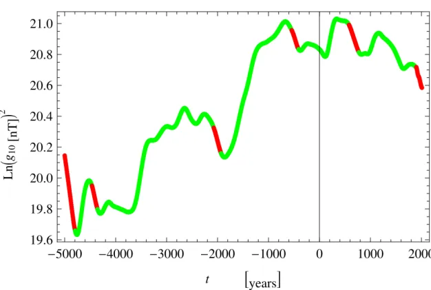
In the data analysis we have used only the term proportional to the dipolar power (g10)2, instead of the term proportional to the total power�n(n + 1) �m(gnm)2+ (hnm)2, for two reasons:

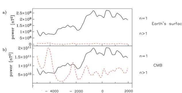
1. If we compare Figure 3.1 and Figure 3.2 we can see that the behaviours of both terms (dipolar and total powers) are similar. This is because CALS7k model probably underestimates gnmwith n > 1.

2. For our aims it is enough to use only g10 because that is the leading term of the total power of the field and it is important for defining the polarity of the magnetic field.

After drawing the graph in Figure 3.1, we supposed that in some temporal intervals, at least longer than 100 years, characterised by a clear dipolar field decay the “dynamo effect”, namely the intensification of the field due to the inductive term of magnetic induction equation, was negligible with respect to the ohmic diffusion of magnetic fields. Therefore, for these intervals (here indicated in chronological order as i=1,...,6) we have supposed, in accordance with the diffusive term of the (3.1), a decay law of this type g10(t) = g10(0)e−t/τi (3.19) with τi= R2 Cµ0σi (k21)2 (3.20)

where τiis the longest dipolar relaxation time of the i-th interval, RCis the outer core radius and k21 is the least non-zero solution of the Bessel function J1/2(x) which is the radial part of the solution of degree n = 1 of the heat equation/diffusive part of the magnetic induction equation; σi is the corresponding apparent electrical conductivity of the core, supposed solid and with the only diffusion process acting. It is for this reason that we call σi"apparent" electrical conductivity. For references about the (3.20) see for example Gubbins and Roberts (1987) or Yukutake (1968) while for references about Bessel functions see for example Abramowitz and Stegun, (1970). From (3.20) we can easily deduce

σi =

τi(k21)2 µ0R2C

3.2 Global models analysis 27 that was used to calculate σifrom each τi.

We performed several fits over the logarithm of the square of g10 coefficient at different values of t; so we have written ln (g10)2vs t in the Figs. 3.1, 3.3 and 3.4; the argument of the logarithm in these graphs is not dimensionless but given in nT2_. In order to estimate the errors on the τiand σiwe bore in mind that the data synthesized by the CALS7k model improve their quality in time, i.e. they are more precise in the recent centuries than in the earlier centuries (De Santis and Qamili, 2010). So we have done the following assumptions on the relative errors on the τi

1. 40% concerning the age 5000 B.C.-4800 B.C. 2. 30% concerning the age 4465 B.C.-4360 B.C. 3. 30% concerning the age 2075 B.C.-1935 B.C. 4. 20% concerning the age 545 B.C.-415 B.C. 5. 20% concerning the age 580 A.D.-770 A.D. 6. 10% concerning the age 1900 A.D.-2010 A.D.

In practice this will mean that relaxation times (and associated errors) and apparent conductivities (and associated errors) are approximated at the closest hundred and thousand, respectively. We have done the same assumptions to perform the simula-tions using CALS3k and CALS10k models (see tables 3.2 and 3.3). In the next pages there are some figures and tables that summarize the results of our analysis.

!5000

!4000

!3000

!2000

!1000

0

1000

2000

19.6

19.8

20.0

20.2

20.4

20.6

20.8

21.0

t

!years"

Ln

#g

$nT

%&

Figure 3.1: ln (g10)2 vs t. The red parts of this graphic represent temporal intervals longer

than 100 years when ln (g10)2 decreased approximately linearly with time; so we

have decided to estimate τiby the data of these intervals. The g10coefficients were

synthesized by CALS7k model except for the last red interval when the coefficients were synthesized by IGRF model.

3.2 Global models analysis 29

Figure 3.2: Temporal trend of the geomagnetic field power on the Earth’s Surface and on the Core Mantle Boundary (CMB)(Figure by Korte and Constable, 2005).

temporal intervals [ years] τi [years] ∆τi[years] σi [S/m] ∆σi [S/m] 5000 B.C.-4800 B.C. (200) 800 300 17000 7000 4465 B.C.-4360 B.C. (105) 1400 400 28000 8000 2075 B.C.-1935 B.C. (140) 1700 500 34000 10000 545 B.C.-415 B.C. (130) 2000 400 42000 8000 580 A.D.-770 A.D. (190) 2100 400 43000 9000 1900 A.D.-2010 A.D. (110) 1700 200 34000 3000 Table 3.1: Relaxation times and apparent electrical conductivities estimated by CALS7k and

IGRF data. Relaxation times (and associated errors) and apparent conductivities (and associated errors) are approximated at the closest hundred and thousand, re-spectively.

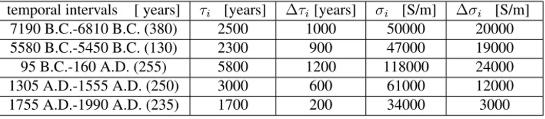
Table 3.2: Relaxation times and apparent electrical conductivities estimated by CALS10k data. Relaxation times (and associated errors) and apparent conductivities (and associated errors) are approximated at the closest hundred and thousand, respectively.

temporal intervals [ years] τi [years] ∆τi[years] σi [S/m] ∆σi [S/m] 7190 B.C.-6810 B.C. (380) 2500 1000 50000 20000 5580 B.C.-5450 B.C. (130) 2300 900 47000 19000 95 B.C.-160 A.D. (255) 5800 1200 118000 24000 1305 A.D.-1555 A.D. (250) 3000 600 61000 12000 1755 A.D.-1990 A.D. (235) 1700 200 34000 3000

!8000

!6000

!4000

!2000

0

2000

20.2

20.4

20.6

20.8

21.0

t

!years"

Ln

#g

$nT

%&

Figure 3.3: ln (g10)2 vs t. The red parts of this graphic represent temporal intervals longer

than 100 years when ln (g10)2 decreased approximately linearly with time; so we

have decided to estimate τiby the data of these intervals. The g10coefficients were

3.2 Global models analysis 31

Table 3.3: Relaxation times and apparent electrical conductivities estimated by CALS3k data. Relaxation times (and associated errors) and apparent conductivities (and associated errors) are approximated at the closest hundred and thousand, respectively.

temporal intervals [ years] τi [years] ∆τi[years] σi [S/m] ∆σi [S/m] 835 B.C.-715 B.C. (120) 1700 300 34000 7000 10 B.C.-100 A.D. (110) 1500 300 30000 6000 260 A.D.-445 A.D. (185) 1600 300 32000 6000 540 A.D.-685 A.D. (145) 1000 200 21000 4000 800 A.D.-915 A.D. (115) 1600 300 33000 7000 1165 A.D.-1275 A.D. (110) 1800 400 36000 7000 1340 A.D. -1440 A.D. (100) 700 100 14000 3000 1565 A.D. -1670 A.D. (105) 1900 400 40000 8000 1755 A.D. -1990 A.D. (235) 1700 200 34000 3000

!1000

!500

0

500

1000

1500

2000

20.6

20.7

20.8

20.9

21.0

21.1

21.2

t

!years"

Ln

#g

$nT

%&

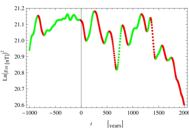
Figure 3.4: ln (g10)2 vs t. The red parts of this graphic represent temporal intervals longer

than 100 years when ln (g10)2 decreased approximately linearly with time; so we

have decided to estimate τiby the data of these intervals. The g10coefficients were

In the table below we report the results from the analysis of SHA.DIF.14k. Table 3.4: Relaxation times and apparent electrical conductivities estimated by SHA.DIF.14k

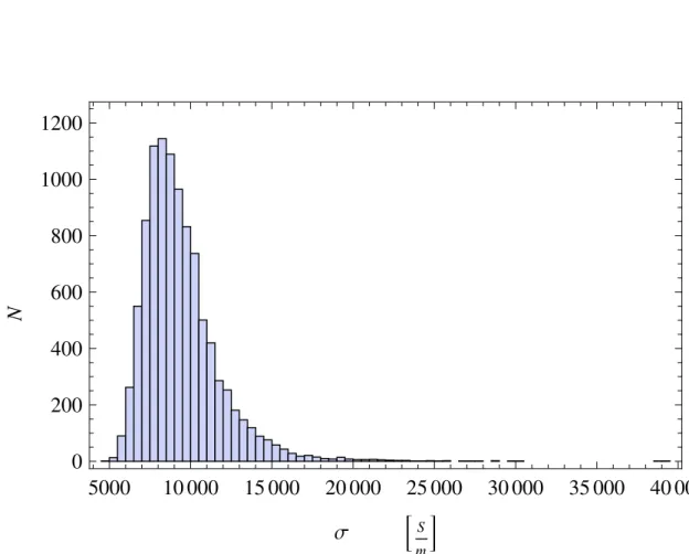
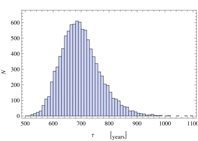
data. Relaxation times (and associated errors) and apparent conductivities (and as-sociated errors) are approximated at the closest hundred and thousand, respectively. temporal intervals [ years] τi [years] ∆τi[years] σi [S/m] ∆σi [S/m] 11200 B.C.-11080 B.C. (120) 500 100 9000 2000

6460 B.C.-6320 B.C. (140) 700 100 14000 1000 1750 A.D.-1875 A.D. (125) 2500 500 50000 10000

We estimated the errors in this table, by a gaussian bootstrap method with 10000 iterations. We used also this gaussian bootstrap method to estimate the errors, because it is a robust method widely used in geomagnetism (See e.g Korte et al., 2011 or Pavón-Carrasco et al., 2014) and there are several articles that highlight the importance of the fact that the statistics of the geophysical data is gaussian (see e.g Constable and Parker, 1988). In the next pages there are some histograms about the relaxation times and the "apparent conductivities" got by the bootstrap method.

3.2 Global models analysis 33

500

1000

1500

2000

2500

0

200

400

600

800

1000

Τ

!years"

N

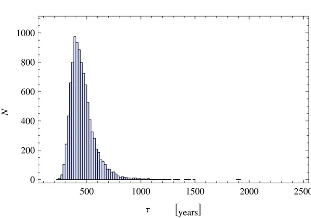
Figure 3.5: Histogram about the 10000 decay times got by a bootstrap method in the age between 11200 B.C and 11080 B.C.

5000

10 000

15 000

20 000

25 000

30 000

35 000

40 000

0

200

400

600

800

1000

1200

Σ

!

"

N

Figure 3.6: Histogram about the 10000 apparent conductivities got by a bootstrap method in the age between 11200 B.C and 11080 B.C.

3.2 Global models analysis 35

500

600

700

800

900

1000

1100

0

100

200

300

400

500

600

Τ

!years"

N

Figure 3.7: Histogram about the 10000 decay times got by a bootstrap method in the age be-tween 6460 B.C and 6320 B.C.

10 000

12 000

14 000

16 000

18 000

20 000

22 000

0

100

200

300

400

500

600

Σ

!

"

N

Figure 3.8: Histogram about the 10000 apparent conductivities got by a bootstrap method in the age between 6460 B.C and 6320 B.C.

3.2 Global models analysis 37

2000

3000

4000

5000

6000

7000

0

200

400

600

800

1000

Τ

!years"

N

Figure 3.9: Histogram about the 10000 decay times got by a bootstrap method in the age be-tween 1750 A.D. and 1875 A.D.

40 000

60 000

80 000

100 000

120 000

140 000

0

200

400

600

800

1000

Σ

!

"

N

Figure 3.10: Histogram about the 10000 apparent conductivities got by a bootstrap method in the age between 1750 A.D. and 1875 A.D.

3.2 Global models analysis 39

!12 000 !10 000

!8000

!6000

!4000

!2000

0

2000

19.5

20.0

20.5

21.0

t

!years"

Ln

#g

$nT

%&

Figure 3.11: Analysis of several Geomagnetic Axial dipoles vs t ; blue lines: g01by sha.dif.14k;

pink lines: strong decays of g01by sha.dif.14k; green lines: g01by cals10k; red

lines: strong decays of g01by cals10k; yellow lines: g01by pfm9k.1; black lines:

strong decays of g01by pfm9k.1; purple line: g01by IGRF12 . (Figure by Filippi et

al., 2015)

Finally we can state that the best value of the apparent core conductivity for the last 7000 years deduced by our study is the average of the σi± the ratio between their standard deviation and√6

σcore= (33000 ± 4000) S/m

By the analysis of the data synthesized by the other CALS model we found con-ductivities of the same order of the conductivity found by the data synthesized by CALS7k. More specifically the conductivity estimated by geomagnetic field synthe-sized by CALS10k is

σcore= (62000 ± 15000) S/m

and the conductivity estimated by the field synthesized by CALS3k is σcore= (30000 ± 3000) S/m

By analyzing the results in the Table 3.4 and the Figures 3.5, 3.7, 3.9, 3.6, 3.8 and 3.10, we can state that also the decay times and the correspondent apparent conductivities are one order of magnitude smaller than the commonly accepted values; in other words we found for the last 14000 years some values of the conductivities smaller than expected

So the found apparent core conductivities for the last 14000 years are, at least, one order of magnitude smaller than the commonly accepted values (see e.g. Gubbins and Roberts, 1987; Stacey and Loper, 2007; Pozzo et al., 2012 and the articles cited in those papers); this fact would have interesting implications as we will explain in Chapter 5 .

Chapter 4

Outer Core Dynamics and rapid

intensity changes

In this chapter we use an interesting large scale method in order to estimate the rapid changes of the dipolar geomagnetic field. This method was developped by P.W. Liv-ermore, A. Fournier and Yves Gallet and it is described in the paper Livermore et al., (2014). We describe this method and then we present the results got by an extension of this method.

4.1 Introduction

The work described in Livermore et al., (2014) gives an estimation of the maximum temporal variation of the Geomagnetic Field in some epochs by the Lagrange multi-pliers technique. The unique constraint assumed is that the root-mean-squared (rms) flow speed on the Core Mantle Boundary (CMB) is 13 km/yr (Holme, 2007). This constraint is a results of several simulations performed on some geomagnetic models. In these models there are two fundamental assumptions:

1. The Geomagnetic Field is in the frozen-flux condition, namely the first term of the R.H.S of the (1.10) vanishes.

2. The flow of the liquid core is tangentially geostrophic, namely ∇H· (v cos θ) = 0, where ∇His the "horizontal divergence" and v is the velocity field of the outer core.

If we consider only short-time intervals, the Frozen-Flux hypothesis is reasonable, be-cause the diffusive effects are more effective after long-time intervals. If the gravity is fully radial the condition about the tangentially geostrophic flow is satisfied. The Outer Core is more spherical than the Earth’s Surface, so it is quite correct to assume that the gravity is fully radial on the CMB. So, we can state that it is a good approximation to assume the constraint that the root-mean-squared flow speed on the Core Mantle Boundary (CMB) is 13 km/yr.

4.2 Methodology

The geomagnetic intensity at S site is given by F =_{|B| =}�B2 r+ Bθ2+ Bφ2 (4.1) so dF dt = 1 F � Br dBr dt + Bθ dBθ dt + Bφ dBφ dt � = 1 F � B ·dB dt � (4.2) If we ignore the diffusion and assume ∇ · v = 0 the radial component of the magnetic induction equation at the CMB (r = c, c = 3485 km) becomes

∂Br

∂t = −∇H· (vHBr) (4.3) where vHis the horizontal flow and ∇H = ∇ − ˆr_∂r∂ , with ˆr is the radial unit vector. Since the main sources of the Geomagnetic Field are in the core, we can represent the B and hencedB

dt as a conservative field for each r ≥ c; by bearing in mind the (3.10), we can formalize these concepts in the following way:

dB dt = −∇ � a ∞ � l=1 l � m=0 � a r �l+1

( ˙glmcos(mφ) + ˙hlmsin(mφ))Plm(cos θ) �

(4.4) We are interested on the temporal evolution of the B field at P site; so we wrote a derivative and not a partial derivative in the equation above. In the (4.4) a is the Earth’s radius, l are the degrees of a Spherical Harmonic expansion, m are the orders of a Spherical Harmonic expansion, ˙glmand ˙hlm are the Gauss coefficients of the secular variation; by the (4.3) and (4.4) we can deduce that these coefficients depend linearly on v, from it follows that all the components of dB

dt at r = a and indeed dF

dt depend linearly on v at r = c. In other words:

dF dt = G

T_{q (4.5)}

Where G is a suitable ad hoc column vector, and q is a vector verifying: v =�

k

qkvk (4.6)

Since the velocity field are divergence-free, the field v can be, in general, expressed as the following sum of the Spherical Harmonic Ym

l (θ, φ): v = ∇ × (tm

l Ylm(θ, φ)r) + ∇H(rsml Ylm(θ, φ)) (4.7) up to a fixed spherical harmonic degree LU, where vk is defined by the vector of coefficients (tm

l , sml ) of zeros except for a one in the k-th position.

For a given site location and prescribed magnetic field (to degree LB), the vector G is then straightforward to assemble, one element at a time. Each mode of flow was taken in sequence, so it is possible to calculate the spherical harmonic spectrum to degree LB+LUof ∂Br/∂tat r = c using a standard transform methodology based on Gauss-Legendre quadrature and fast-Fourier transform; then using (4.4) it is possible

4.2 Methodology 43 to obtain the the contribution to dF/dt at S; so it is possible to deduce the elements of G. The "mean-squared velocity" on a sphere can be written in this way:

qT_{Eq =} 1 4π � l,m (l + 1)�(tm l ) 2_{+ (s}m l ) 2� 4π 2l + 1 (4.8)

E is a diagonal matrix with elements l(l + 1)(2l + 1)−1_{. If we bear in mind the} important constraint on the rms on the CMB and the (4.8) we can evaluate the q (and so the v) that maximizes the dF/dt by the Lagrangian multipliers technique, namely

dF dt � � � �_max= maxq � GT_{q − λ(q}T_Eq − T2 0) � (4.9) where λ is the Lagrange multiplier and T0is the root-mean-squared (rms) velocity on the CMB: T0= � 1 4π � r=c|v| 2_{dΩ (4.10)}

dΩis the infinitesimal solid angle and the integral in the (4.10) is taken over the surface of the outer core.

At a local maximum, the gradient of the function GT_{q − λ(q}T_{Eq− T}2

0) with respect to each component of the vector q is zero, so we can define the "qmF v":

qmF v= 1

2λE−1GT (4.11)

where λ is found by scaling the flow to the target rms. The inclusion of magnetic diffusion is a simple extension of the above methodology, indeed we can write

∂Br

∂t = −∇H· (vHBr) + ηˆr · ∇

2_{B (4.12)}

where η is the magnetic diffusivity already defined in the previous chapters. Since Since B is assumed known, the second term of the R.H.S. of the (4.12) does not depend on v; so, it has no no bearing on the optimising flow.

This approach, maybe, could be useful for understanding whether some very rapid changes in the intensity of the Earth’s Magnetic Field are consistent with a model of the source region of the magnetic field, namely the fluid flow at the surface of Earth’s outer core. In this regard it is worth to remind that some recent works suggest that extremely rapid fluctuations in the Earth’s Magnetic Field have occurred in the past (see e.g. Ben-Yosef et al., 2009, Shaar et al., 2011 or Gómez-Paccard et al., 2012). The maximum variation of the instensity of the geomagnetic field estimated by Livermore et al., (2014) is consistent with the study performed by Gómez-Paccard et al., (2012), but not with the studies performed by Ben-Yosef et al., 2009 and Shaar et al., 2011. However this second case may be due to the fact

We modify the program used by Livermore et al., (2014), in order to get a program that estimates the maximu of the temporal derivative of the g01Gauss coefficient during several ages. In the next page there are some figures that summarize the results of our analysis. We analyzed a small temporal interval, because during these short ages it is reasonable assuming the constraint that the root-mean-squared (rms) flow speed on the Core Mantle Boundary (CMB) is 13 km/yr, but probably it is possible to extend the analysis, at least, for a time interval between 1900 A.D. to 2015 A.D

1980

1985

1990

1995

2000

2005

2010

2015

120.5

121.0

121.5

122.0

122.5

t

!years"

Max

#

dg

dt

$!

nT

%y

"

Figure 4.1: Maximum temporal variation of g01in the ages between 1980 A.D. and 2015 A.D.

4.2 Methodology 45

1980

1982

1984

1986

1988

1990

121.8

122.0

122.2

122.4

t

!years"

Max

#

dg

dt

$!

nT

%y

"

Figure 4.2: Maximum temporal variation of g01in the ages between 1980 A.D. and 1990 A.D.

1980

1982

1984

1986

1988

1990

121.8

122.0

122.2

122.4

t

!years"

Max

#

dg

dt

$!

nT

%y

"

Figure 4.3: Maximum temporal variation of g01in the ages between 1980 A.D. and 1990 A.D.

(these coefficients are by CALS3k model (For reference about this modelKorte and Constable, 2003 and Korte et al., 2009))

Chapter 5

Discussion and Conclusions

In this thesis we deal with some aspects of the Dynamo Theories. In the Chapter 3, we looked for a connection between the recent trend of the geomagnetic field and the turbulent dynamo theories. The models of the geomagnetic field of the last 3000, 7000, 10000 and 14000 years show a field that has intermittent decays so that the magnetic diffusivity would correspond to a value of conductivity much smaller than the most commonly accepted value. If we compare Figs. 3.1, 3.3 and 3.4, we can see that there is no contemporary turbulent diffusive behaviour in the different studied models; in fact the exponential decays of the dipole field occur in different epochs for different models. However, as we can check by the tables 3.1, 3.2 and 3.3, almost all apparent electrical conductivities are one order of magnitude smaller than the commonly accepted values, that are probably more correct than ours. In other words, all models show that when the geomagnetic dipolar field decays it does with a rate faster than the typical diffusive rate so we can speculate that this is a general feature of the geomagnetic field of the last millennia. This is due to the presence of an additional term β in the diffusion part (see eq.(3.8)), so we can call this process a "turbulent diffusive" regime of the recent geomagnetic field. This "turbulent diffusivity" is probably due to the turbulence effects in the core and accelerates the process of field decay (according to the (3.8)). This tur-bulent diffusivity would explain why our conductivity values, obtained neglecting the inductive term in (3.1), are one order of magnitude smaller than the expected values for the core. In this regard, we recall that 5 × 105_{S/m, a value we find quite often in the} literature (see e.g. Gubbins and Roberts, 1987 and also Stacey and Anderson, 2001) and 2.76 × 105_{S/m (that is a more recent estimate performed by Stacey and Loper,} 2007), are approximately one order of magnitude greater than our σi. This turbulent diffusivity, in turn, could eventually bring the planetary magnetic field toward a field reversal in a sort of avalanche process, typical of a turbulent, and occasionaly chaotic, regime. This turbulent diffusive effect, as we will see in the Appendix A, is greater in case of a isotropic, homogeneous and mirror-symmetric turbulence. This is coherent with some other papers (see for example De Santis, 2007 or Hulot et al., 2002, which are based on fully different approaches) that suggest that an imminent magnetic field reversal is possible (about 1000 or 2000 years from now). Also the article of Liu and Olson (2009) could support our hypothesis; in fact it reminds the very fast decrease of the geomagnetic dipole moment in the last 160 years (at least one order of magnitude faster than the free decay rate) and emphasizes that the process of advective mixing in the core can enhance the magnetic diffusion. There are also other articles that show that the geomagnetic dipole moment has recently decayed with a rate faster than the typical

diffusive rate (see e.g. Gubbins et al., 2006 and other references here cited). However most of this works speak about the last century or the last 4 centuries. Instead, our results show a turbulent diffusive regime regime which lasts for at least 14000 years. This, in our opinion, strengthens the hypothesis that the recent geomagnetic field is in a turbulent diffusive regime. Furthermore, there is a paleomagnetic study described in Nowaczyk et al. (2012) that shows that the Laschamp excursion occurred in a time much shorter than the time corresponding to the free decay rate due to the ohmic diffu-sion of the geomagnetic field. In fact the record relating to this excurdiffu-sion, shows a full polarity reversal, although temporary, that lasted for about 200 years; the whole pro-cess, namely from the beginning when there was the current geomagnetic polarity until the end, when there was again the current geomagnetic polarity, lasted for about 3600 years, a time comparable to the relaxation times estimated by us from the geomagnetic global models. Therefore, an excursion, and so probably also a polarity reversal, would occur in a time faster than the time corresponding the typical magnetic diffusivity. This experimental observation could suggest that before an excursion or reversal there is a turbulent diffusive regime. For some details about the Laschamp excursion see the ar-ticle of Nowaczyk et al. (2012). Of course, because of the limited number of cases here analysed, further studies will be necessary to establish if the hypothesis of the turbulent diffusivity for the recent geomagnetic field is correct or not. This could be verified in several ways. For instance, we could try to estimate some other important geophysical parameters such as, for example, the β coefficient in the eq. (3.8). In fact, as it is shown in the Appendix A, this coefficient is connected with |v|2_{. In other} words we could do some more accurate estimations of other important parameters, or use some values reported in other woks, to try to solve the magnetic induction equation under less restrictive assumptions and then compare the results with those of previous works (e.g. with the Glatzmaier-Roberts dynamo described in Glatzmaier and Roberts (1995a; 1995b)) and with experimental data. More specifically, it will be worth trying to solve the (3.9) or more simplified expressions (for example we can assume that |v|2 is uniform and constant or that c(00)_{� a}(00)_{and c}(00)_{� a}(01)_{). Furthermore we could} try to estimate the terms O(|v|3_{) or O(|v|}4_{) of ∆ (for more details see the Appendix} A). In this manner we may find a solution of the magnetic field less approximate than the solution of the diffusive part of the (3.1) and we can, by simple numerical simu-lations, compare these results with experimental data. Moreover we could repeat our analyses on some regional models; so we can verify if there are some turbulent diffu-sive behaviours limited to more restricted regions. This would be important because there are some regions where the geomagnetic field decays more quickly than in others and there also some regions where it seems that the magnetic field doesn’t decay at all (Gubbins, 1987). So we could try to understand if the turbulent diffusivity is also space dependent.

There are several arguments that suggest that the turbulent diffusivity may be an important component of any possible magnetic field reversal. In fact if the inductive term disappears, the decay times will be about 10000 years instead of about 1000-2000 years as it reported in several papers (see e.g. Liu and Olson, 2009 or Hulot et al., 2002). But if the inductive term vanishes, maybe the magnetic field will not regener-ate itself. So we think that a better understanding of the turbulence in the core can be useful to improve our knowledge about the generation, extinction and regeneration of the geomagnetic field. On the other hand, several authors believe that the geomagnetic polarity reversal might be connected with a magnetic flux of opposite sign in the south-ern hemisphere (see e.g. Gubbins, 1987); so we could try to compare these types of studies with our studies on the turbulent diffusivity of the geomagnetic field. Another

49 interesting aspect of the dynamo theories is the role of the symmetries as explained for example in Rädler (1968a) or in Merrill et al. (1996). We think that these studies could be useful to understand better some aspects of the dynamics of the Earth’s Magnetic Field, that has several features not well-understood yet.

It is interesting to note, by analyzing the Figures 4.1, 4.2 and 4.3 that when the dipolar geomagnetic field exponentially decay its temporal derivative linearly decrease. Maybe it could be interesting to do other analysis with simulations or during real situations, in order to check whether this feature is verified before a polarity reversal or excursion.

Appendix A

Calculation of the mean

electromotive force

In this appendix we will give some details on the calculation of the mean electromotive force within suitable approximations. We will perform some manipulations in a sim-ilar way as was already done by different authors (see Moffatt, 1978; Rädler, 1968a; 1968b).

To discuss the term ∆ in (3.6) and (3.7) we need, at least, a formal solution of the (3.7); so we assume that V = V0, v, B0= B and (for the moment) C are known and we rewrite the (3.7) in tensor notation1

η_∇2bi+ εimnεnpq ∂ ∂xm � Vpbq�− ∂bi ∂t = −εimn ∂ ∂xm � εnpqvpBq+ Cn) (A.1) We may solve (A.1) with a suitable boundary condition on b(r, t0) in the form

bi(r, t) = � Gil(r, t; r�, t0)bl(r�, t0)dr�+ +� � t t0 Gil(r, t; r�, t�)εlmn ∂ ∂x� m � εnpqvp(r�, t�)Bq(r�, t�) + Cn(r�, t�)�dr�dt� (A.2) where Gil(r, t; r�, t�) is a suitable function that satisfies the following properties

η_∇2rGil+ εimnεnpq ∂ ∂xm � VpGql � −∂G_∂til = −δilδ(t− t�)δ(r − r�) (A.3) Gil(r, t; r�, t�) → 0, for |r − r�| → +∞ (A.4) Gil(r, t; r�, t�) → δilδ(r− r�), for (t − t�) → 0 (A.5) the expression ∇2 rGil(r, t; r�, t�) means�_j ∂ 2 ∂x2jGil(r, t; r

�_{, t}�_{) and the integrals with} no end points of integration, like�dr�in the (A.2), are, of course, integrals that must

1_{In this appendix we adopt the Einstein summation convention everytime we write two repeated indices}