Molluscs of the marine protected area "Secche di Tor Paterno"

(1)

A

l

m

a

M

a

t

e

r

S

t

u

d

i

o

r

u

m

–

U

n

i

v

e

r

s

i

t

à

d

i

B

o

l

o

g

n

a

DOTTORATO DI RICERCA IN

BIODIVERSITA’ ED EVOLUZIONE

Ciclo XXIII

Settore scientifico-disciplinare di afferenza: BIO/05 ZOOLOGIA

MOLLUSCS

OF THE MARINE PROTECTED AREA “SECCHE DI TOR PATERNO”

Presentata da:

Dott. Paolo Giulio Albano

Coordinatore

Dottorato

Relatore

Prof.ssa Barbara Mantovani

Prof. Francesco Zaccanti

Co-relatore

Prof. Bruno Sabelli

(2)

(3)

to Ilaria and Chiara, my daughters

This PhD thesis is the completion of a long path from childhood amateur conchology to scientific research. Many people were involved in this journey, but key characters are three.

Luca Marini, director of “Secche di Tor Paterno” Marine Protected Area, shared the project idea of field research on molluscs and trusted me in accomplishing the task. Without his active support in finding funds for the field activities this project would have not started. It is no exaggeration saying I would not have even thought of entering the PhD without him.

Bruno Sabelli, my PhD advisor, is another person who trusted me above reasonable expectations. Witness of my childhood love for shells, he has become witness of my metamorphosis to a researcher.

Last, but not least, Manuela, my wife, shared my objectives and supported me every single day despite the family challenges we had to face.

Many more people helped profusely. I sincerely hope not to forget anyone.

Marco Oliverio, Sabrina Macchioni, Letizia Argenti and Roberto Maltini were great SCUBA diving buddies during field activities.

Betulla Morello, former researcher at ISMAR-CNR in Ancona, was my guide through the previously unexplored land of non-parametric multivariate statistics.

Philippe Bouchet and Philippe Maestrati, Muséum National d'Histoire Naturelle (Paris), were welcoming and helpful during my work with them. Navigating through 23.000 specimens of Indo-Pacific triphorids from their research campaigns has been an experience I will never forget. It is rare to have so much material of excellent quality to study. I have been able to touch biodiversity first hand.

Paolo Vestrucci and Roberto Colzani manage NIER Ingegneria Spa. Working with this company allowed the first contacts and activities with the Marine Protected Area which then developed into the survey that gave most of the data for this thesis.

Paolo Giuntarelli, former director of the public body RomaNatura which manages the Marine Protected Area, kept on the work done by Luca Marini in safe-guarding funds for the field activities during Luca’s absence.

Paolo & Marisa, Gabriella & Vincenzo were great in helping me combining work and family. Moreover, Gabriella was supportive and was one of the people who shared my objectives most.

Francesca Evangelisti, Eimi Ailen Font, Michela Kuan, Wanda Moshfegh, Linda Tragni, Francesca Orrù, Maria Teresa Greco helped sorting samples out in the field or in laboratory.

Anna Maria Candela, Department of Matematics, University of Bari, helped reviewing the English of some mathematical methodological parts.

Mirco Travaglini and Stefania Brunetti, Library of the Department of Experimental Evolutionary Biology, helped in locating and obtaining literature.

Further help during these three years has been given by Francesco Criscione, Carlo Froglia, Maria Cristina Gambi, Giuliana Gillone, Virginie Héros, Susan M. Kidwell, Constantine Mifsud, Stefano Palazzi, Paul Sammut, Cristiano Solustri, Helmut Zibrowius.

(4)

Key-words: Mollusca, ecology, biodiversity, conservation, Posidonia oceanica, coralligenous, detritic pools, Secche di Tor Paterno

(5)

1

1 Index

1 Index ... 1

2 Executive summary ... 5

2.1 The molluscan diversity... 5

2.2 Biocoenoses characterization ... 5

2.3 Analysis of the Posidonia leaves species assemblage ... 5

2.4 Analysis of the Posidonia rhizomes species assemblage ... 6

2.5 Analysis of the coralligenous species assemblage ... 6

2.6 Analysis of the detritic species assemblage ... 7

2.7 Agreement between death and living assemblages ... 7

3 Introduction ... 9

3.1 The studied area ... 9

3.2 Why sampling in a marine protected area?... 11

3.3 The molluscan fauna ... 11

3.4 Abbreviations ... 12

4 Materials and methods ... 13

4.1 Field activity ... 13

4.2 Laboratory sorting ... 15

4.3 Data analysis techniques ... 15

4.3.1 Standardisation ... 16

4.3.2 Transformation ... 16

4.3.3 Similarity matrix ... 16

4.3.4 One-way ANalysis Of VARiance (ANOVA) ... 17

4.3.5 Mann–Whitney U test ... 18

4.3.6 Cluster analysis ... 18

4.3.7 Non-metric Multi-Dimensional Scaling (MDS) ... 19

4.3.8 Multivariate ANalysis Of SIMilarities (ANOSIM) ... 19

4.3.9 SIMilarity PERcentage breakdown (SIMPER) ... 20

4.3.10 PERmutational Multivariate ANalysis Of VAriance (PERMANOVA) ... 21

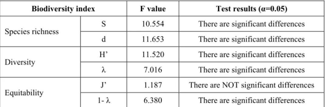
4.4 Biodiversity indices ... 21

4.4.1 Number of species (S) ... 21

4.4.2 Number of specimens (N) ... 22

4.4.3 Margalef’s species richness (d) ... 22

4.4.4 Shannon index (H’) ... 22

4.4.5 Equitability (J’) ... 22

4.4.6 Simpson index (λ) ... 22

4.5 Biodiversity estimators ... 23

4.6 Trophic groups and feeding guilds ... 23

4.7 The role of species in describing biocoenoses ... 24

5 Sampling results and efficacy ... 25

5.1 Results ... 25

5.2 Discussion ... 29

(6)

2

6.1 Results ... 30

6.1.1 Faunal list ... 30

6.1.2 Biocenotic preferences ... 34

6.2.1 Biodiversity of the malacofauna and its interest for conservation ... 39

6.2.2 Biocenotic preferences ... 43

7 Biocoenoses characterization ... 45

7.1 Results ... 45

7.1.1 Univariate approach ... 45

7.1.2 Multivariate approach ... 54

7.1.3 Analysis with other phyla ... 67

7.1.3.1 Errant Polychaeta ... 67

7.1.3.2 Crustacea: “crabs” (suborder Pleocyemata) ... 69

7.1.3.3 Brachiopoda ... 70

7.2.1 Molluscs ... 71

7.2.2 Other phyla ... 73

8 Analysis of the Posidonia leaves species assemblage ... 74

8.1 Results ... 74

8.1.1 Posidonia oceanica bed structure and morphometry ... 74

8.1.2 The molluscan community ... 76

8.1.3 Mollusca community structure ... 78

8.1.4 Comparison with other data sets ... 80

8.1.4.1 Secche della Meloria (Livorno) ... 82

8.1.4.2 Elba Isl. ... 84

8.1.4.3 Giglio Isl. ... 87

8.1.4.4 Ischia Isl. ... 90

8.1.4.5 Hvrgada Isl, Croatia ... 93

8.1.4.6 Comparison between localities ... 96

8.2.1 Secche di Tor Paterno community ... 100

9 Analysis of the Posidonia rhizomes species assemblage ... 104

9.1 Results ... 104

9.1.1 Posidonia oceanica bed structure and morphometry ... 104

9.1.4.1 Secche della Meloria (Livorno) ... 119

9.1.4.2 Elba Isl. ... 123

9.1.4.3 Giglio Isl. ... 130

9.1.4.4 Hvrgada Isl., Croatia ... 135

(7)

3

10 Analysis of the coralligenous species assemblage... 148

10.1 Results ... 149

10.1.1 Habitat description ... 149

10.1.4.1 Secche di Tor Paterno ... 172

10.1.4.2 Capo San Marco, Sciacca (Agrigento) ... 176

10.1.4.3 Riserva Orientata dello Zingaro, Scopello (Trapani) ... 182

11 Analysis of the detritic species assemblage ... 192

11.1 Results ... 192

11.1.1 Habitat description ... 192

11.1.4.1 Secche di Tor Paterno 2004 (Univ. Tor Vergata) ... 197

11.2.2 Comparison with othet data sets ... 206

12 Agreement between death and living molluscs assemblages ... 207

12.1 Materials and methods ... 208

12.1.1 Material studied ... 208

12.1.2 Sediment analysis ... 208

12.1.3 Biocoenoses data adjustments ... 209

12.1.4 Data analysis ... 210

12.1.5 Metrics to evaluate the fidelity between the death and living assemblages ... 210

12.2 Results ... 211

12.2.1 Experiment repeatability ... 211

12.2.2 Sediment minimum volume ... 211

12.2.3 Sediments species composition ... 212

12.2.4 Comparison between biocoenoses and thanatocoenoses ... 217

12.2.4.1 Qualitative biodiversity comparison ... 217

12.2.4.2 Fidelity with respect to species richness and taxonomic composition ... 218

12.2.4.3 Species assemblages comparison ... 220

12.2.4.4 Fidelity with respect to species dominance ... 226

12.3.1.1 Experiment repeatability ... 228

12.3.1.2 Sediment minimum volume ... 228

(8)

4

12.3.1.4 Comparison between biocoenosis and thanatocoenosis ... 228

12.3.1.5 Fidelity with respect to species richness and taxonomic composition ... 229

12.3.1.6 Species assemblages comparison ... 231

12.3.1.7 Fidelity with respect to species dominance ... 231

(9)

5

2 Executive summary

This thesis was aimed at describing the molluscan biodiversity of the infralittoral off-shore reefs in the “Secche di Tor Paterno” marine protected area. Off-shore reefs are a rather common feature of the Mediterranean Sea submarine landscape constituted by outcrops of hard substratum emerging from wide open soft substrata.

Four biocoenoses were sampled by SCUBA diving: Posidonia oceanica leaves and rhizomes, coralligenous concretions and detritic pools. The malacofauna of each biocoenosis was studied in detail. Moreover, comparison data sets from other localities and depths were used as comparison material to further understand the patterns of diversity. Polychaeta, Pleocyemata (Crustacea) and Brachiopoda were studied at different degrees of detail with the final aim to understand to which extent different taxonomic groups worked well as descriptors of biocoenoses and therefore if molluscs were a reasonable or optimal choice.

The thanatocoenoses near the biocoenoses were sampled too to assess the agreement between the death and life assemblages.

The main conclusions of this thesis are given in the following paragraphs.

2.1 The molluscan diversity

The high habitat heterogeneity of the reefs allows the establishment of a highly diverse mollusc assemblage: 162 species were found alive and a good number of them live exclusively in given biocoenoses. The sampled fauna is 9% of the Italian fauna and 15% of the fauna of the biogeographic sector 2. These numbers are very high considering the geographic restrictness of the area, the narrow depth interval which implies that several biocoenoses are not present (e.g. photophilous algae, deep water corals), the lack of true soft substrata, the single season and single year sampling and that a 1 mm sieve was used (so missing some tiny species like Pyramidellidae). Moreover, biodiversity estimators suggest that the total richness of species may reach 236 species (second order Jackknife 2 estimator).

The coralligenous proved to be the richest biocoenosis both in terms of total number of species (123) and species living exclusively there (53). The Posidonia rhizomes are the second richest biocoenosis (88 species). The Posidonia leaves were rather poor with just 14 species and the detritic pools host 22 species. However, these two biocoenoses contributed with a good share of species not found elsewhere. This is particularly remarkable for the detritic pools: 13 species (59.1%) were found in this biocoenosis only. The reefs host 4 species of conservation interest: Erosaria spurca and Luria lurida (Gastropoda: Cypraeidae),

Lithophaga lithophaga (Bivalvia: Mytilidae), Pinna nobilis (Bivalvia: Pinnidae). No alien species were

found on the reefs.

The high habitat and species diversity of these reefs, the presence of species of conservation interest and the lack of alien species, pooled with their distance from the coastline which implies less intense anthropogenic impacts suggest the need of a greater effort for the protection and conservation of this kind of submarine structures.

2.2 Biocoenoses characterization

The a priori choice of molluscs as descriptors of biocoenoses was confirmed by their good behaviour in discriminating even similar biocoenoses like the coralligenous and Posidonia rhizomes since the molluscan assemblages of the biocoenoses are significantly different (PERMANOVA, p<0.05). Errant Polychaeta, Pleocyemata (Crustacea) and Brachiopoda did not show significantly different communities in these two biocoenoses.

The power of molluscs may be in their high species diversity and low vagility. Despite this analysis has some limitations due to samples preservation and taxonomic challenges of polychaetes and crabs, this is the first attempt of such a comparison in Mediterranean complex hard substratum environments.

2.3 Analysis of the Posidonia leaves species assemblage

Despite the Posidonia leaves fauna has been studied several times, information about deep water meadows (below 15 m) is scarce.

(10)

6

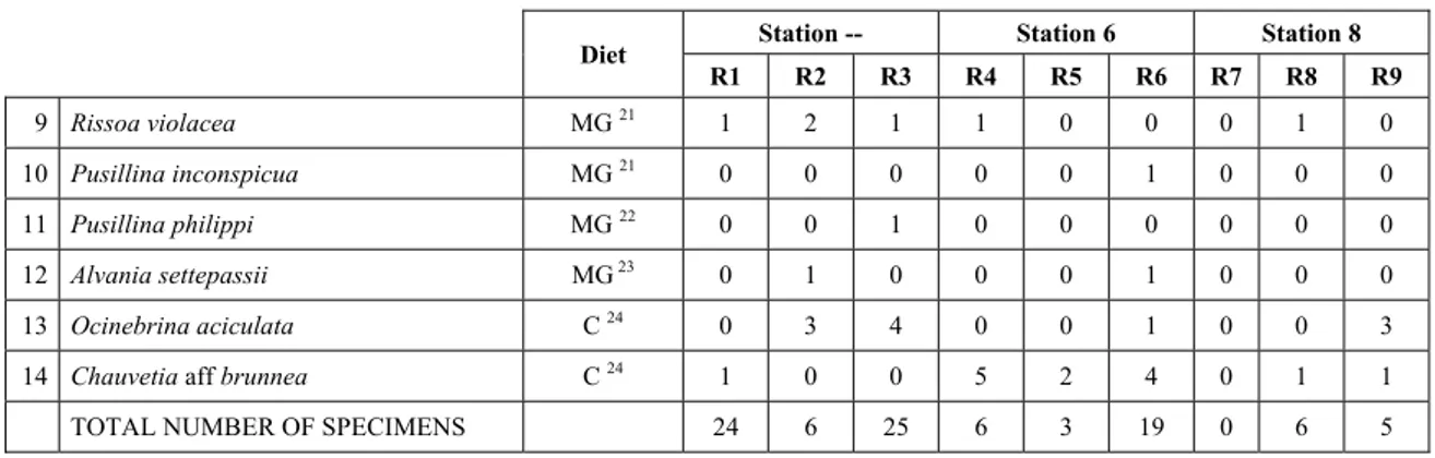
In “Secche di Tor Paterno” the Posidonia leaves species assemblage is characterized by its poorness. Only 14 species were collected. Moreover, species which usually thrive in this biocoenosis were found in very limited quantity (e.g. Bittium latreillii, Jujubinus exasperatus, Rissoa auriscalpium, the latter however prefers shallower meadows) or were absent (e.g. Smaragdia viridis, a few specimens were found in the rhizomes). The leaves stratum hosts however some interesting species due to their spotty distribution (Chauvetia aff brunnea) or restricted range (Alvania settepassii). No significant differences could be recognized between assemblages living on Posidonia settled on different substrata (soft vs hard) and this is consistent with the lack of significant differences of shoot density which is the main Posidonia bed structure parameter. Most of the characteristic species described by Pérès & Picard (1964) are present (e.g.: Jujubinus

exasperatus, Rissoa auriscalpium, Rissoa violacea, Pusillina philippi, Bittium latreillii, Ocinebrina aciculata

and Chauvetia aff. brunnea).

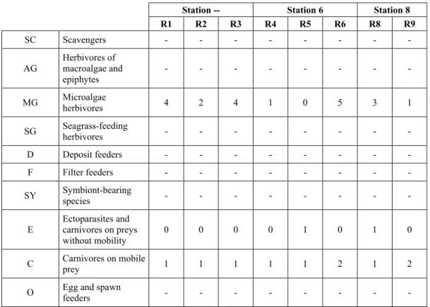
This community is dominated by microalgae herbivores both in terms of number of specimens and species. However, carnivores may be a very important component being present up to 83.3% of the total number of specimens within a single replicate as already described for other deep water .

Comparison with data sets from other localities suggest that deep water (below 15 m) communities are significantly different from shallower water ones in terms of species composition and abundance. Due to this issue, the variation of the community across geographic gradients couldn’t be investigated satisfactorily.

2.4 Analysis of the Posidonia rhizomes species assemblage

The malacocoenosis of the Posidonia rhizomes is rich and diversified. Eighty-eight species were collected. Several species are rare and of deep water affinity like Hanleya hanleyi, Obesula marisnostri, Mathilda

gemmulata. Almost a third of the community is composed by carnivores and 24.1% of the species are

specialized carnivores on preys without mobility (Fissurellidae, Triphoridae, Cerithiopsidae, Eulimidae, Pyramidellidae) and this enhances diversification and rarity. Microalgae herbivores are a fourth of the assemblage and another fourth is made by filter-feeders.

Posidonia oceanica settles in the Secche di Tor Paterno reefs on two different substrata: hard coralligenous

concretions and small sedimentary pools. The two assemblages are not significantly different, however those living on soft substratum have an high presence of infaunal species.

Comparison with other data-sets further supports the hypothesis that the rhizome layer of Posidonia hosts a rich molluscan community, much richer than the leaves stratum, and with reduced dominance phenomena. Despite the ubiquitous Bittium latreillii dominates 60% of studied samples, the other 40% show a wide array of dominant species.

To maximize the sampling success in this environment both defoliation and a wide area (1 m2_{) is suggested.}

2.5 Analysis of the coralligenous species assemblage

In terms of species diversity, the coralligenous hosts the richest species assemblage with 123 species, 77.4% of the whole Secche di Tor Paterno fauna. The richness of the coralligenous is due to the richness of niches and interactions. The mixture of hard substrata and soft enclaves, the richness of sessile species (sponges, gorgonians,…), the sciaphilous conditions help creating the most suitable conditions for boosting molluscan diversity. Several species are rare or of deep water affinity: Danilia tinei, Obesula marisnostri, Cerithiopsis

nofronii and Typhinellus labiatus. Lima lima and Manupecten pesfelis, both considered characteristic species

of the biocoenosis in the literature were found here too.

The coralligenous stations seem to host a rather homogeneous assemblage without significant differences between samples and stations. The biocoenosis is dominated by microalgae herbivores, but carnivorous are an important part of the community and one of the reasons for such a high diversity.

Comparison with other data sets is biased by the great difference in the sampling technique. However, right on this issue it is possible to draw some conclusions. The air-lift sampler performed very well when the number of species and specimens intercepted is concerned. However, it does not manage to sample cemented species (e.g.: Vermetidae, Chamidae, Spondylidae) and may undersample species firmly attached to the substratum (e.g. Striarca lactea, Hiatella arctica, Brachiopoda). Scraping allowed to sample these taxa, but its representation of the biodiversity is lower and the damage to the substratum much higher. Moreover, the air-lift sampler manages to sample better the sediment enclaves in the coralligenous.

(11)

7

2.6 Analysis of the detritic species assemblage

Detritic pools within the reefs may be ascribed to the coastal detritic biocoenosis (DC; Pérès & Picard, 1964). The detritic pools host a poor species assemblage, 22 species, however most of them are exclusive of these soft substrata and these samples have added several species to the knowledge of the malacofauna of the reefs. The only typical molluscan species cited by Pérès & Picard (1964) for this biocoenosis and sampled in the Secche di Tor Paterno pools is Crassopleura maravignae.

Specialized carnivores contribute to the biodiversity with a high number of species, up to 40%. Remarkably, bivalves and filter feeders are not dominant despite soft substrata are usually a suitable environment for them.

The comparison with data sets from the soft substrata around the reefs and within the boundaries of the Marine Protected Area show that the two assemblages are remarkably different. However, when the analysis is run to understand differences between biocoenoses, the coastal detritic station sampled by Università Tor Vergata is the only without statistically significant differences from the detritic pools confirming the hypothesis that this peculiar environments belong to this biocoenosis, despite it probably represents a different and still to be described facies.

2.7 Agreement between death and living assemblages

The analysis of the agreement between death and living assemblages is of interest both in paleoecological reconstruction and in biodiversity conservation, since it could allow the assessment of the biodiversity of an area with a reduced effort and with the advantage of analyzing a time-averaged assemblage which sums up the contribution of several seasons and years.

The study has been carried out by a qualitative comparison of samples from the death and living assemblages, with standard metrics and multivariate techniques. The minimum volume for a meaningful analysis has been evaluated in 1 liter of sediment. The analysis was carried out both with the complete data set and with a reduced one with only those species which contribute more than 1% to the overall abundance. The comparison between living and death assemblages showed that there is a high representativeness of sediments in respect of nearby biocoenoses as a result of low bottom transport. It is important to specify that the spatial scale is in the meters or a few tens of meters. This is supported by:

‐ the neat differentiation of the death assemblages nearby different biocoenoses both by a taxonomic and quali-quantitative point of view, despite being spatially close to other biocoenoses

‐ the taxonomic composition of sediments which is strongly influenced by the living communities (e.g. reduced presence of species of the coralligenous endobenthos in the Posidonia assemblage) ‐ The decrease in the values of some fidelity metrics if the full biocoenoses data set is considered

instead of only data from the stations nearest to the sediment collection sites

Sediments contain some allochthonous species which thrive in the soft substrata around the reefs (mainly bivalves) and some species which couldn’t be intercepted in the biocoenoses survey due to the little destructive sampling techniques used (e.g. endobenthos species, cementing species). When evaluating the biodiversity of the area, the former should be put apart while the latter are an important addition to the knowledge of the area.

Fidelity metrics suggest a good agreement between the living and death assemblages when species richness and taxonomic composition are considered. However, metrics values have to be evaluated in the context of highly diverse molluscan assemblages with little dominance phenomena quite different from those proper of soft substrata which were studied in a number of cases in literature and also different from the few hard substratum cases in literature which focus on a small number of species due to the choice to select only species above 1 or 2 cm in size.

The study suggests that fidelity is lower when considering the species dominance where important differences are described between the living and death assemblages. These differences could be associated to the trophism of species and possibly to the species life span.

(12)

8

The interpretation of recent and fossil thanatocoenoses is seriously affected by the lack of appropriate knowledge on molluscs life histories. Detailed in formation on diets, seasonality, pluriennial variability of populations and information on life spans of species are keys for a full comprehension of biocoenoses dynamics and their contribution to death assemblages. Reversely, fossil death assemblages need this information for their interpretation in a paleoecological perspective.

The study results will help in a better interpretation of paleontological data and foresee good potentialities for the monitoring of biocoenoses using nearby death assemblages. When the latter is considered, the limited diving bottom time required to sample sediments in respect to biocoenoses and the limited field time for treating samples after collection and before laboratory would allow faster surveys and/or greater spatial resolution of sampling. Moreover, the time-averaging effect allows a better description of the fauna, which can be surrogated only by multi-season, pluriennal biocoenoses surveys. However, dead specimens tend to loose important diagnostic characters and may require more skilled personnel for sorting and identification. Another evident drawback of this technique is the limitation to taxa leaving post-mortem remains. Mollusca, however, is the most diverse benthic phylum and therefore allows a good description of the biocoenoses.

(13)

9

3 Introduction

3.1 The studied area

The Marine Protected Area “Secche di Tor Paterno” lies in the Central Tyrrhenian Sea, off the coasts of Lazio (Fig. 1). It is an off-shore reef 12 miles off the coast. The top of the reef is at -18 m, its maximum depth is around -70 m where muddy substratum is found.

It is part of a wider set of off-shore reefs (Fig. 2), made of three main reefs. The “Secche di Terra” are the nearest to the coast and the most shallow, ranging in depth from a few metres to 18-20 metres. The “Secche di Mezzo” are those within the borders of the Marine Protected Area. The “Secche di Fuori” lie on a bottom of a hundred meters deep.

Fig. 1 – Location of the Marine Protected Area “Secche di Tor Paterno” in the Central Tyrrhenian Sea. Lido di Ostia is just south of the river Tevere estuary, which flows through Rome.

(14)

10

Fig. 2 – Bathimetry of the area. The “Secche di Fuori” are too off-shore to be illustrated here. The image is orientated northwards, different shades of colour represent different depths. (courtesy Nautilus Società Cooperativa)

This area is of great conservation interest for several reasons.

First, it is the only Italian marine protected area totally off-shore, without any coastal zone. It is therefore a peculiar conservation experiment and its fauna and biology may be representatives of other off-shore reefs which do not enjoy any kind of protection.

Secondly, it hosts two important benthic biocoenoses: the coralligenous and Posidonia meadows.

The former are calcareous formations of biogenic origin typical of Mediterranean benthic environments, produced by the accumulation of encrusting algae growing in dim light conditions which host several associations and facies. This habitat is considered important for conservation by the Protocol Concerning Specially Protected Areas and Biological Diversity in the Mediterranean of the Barcelona Convention. Relini (2002) considers most of the associations and facies of the coralligenous remarkable or extremely important for conservation purposes.

The latter consists in meadows of the endemic Mediterranean seagrass Posidonia oceanica ((L.) Delile, 1813). It is an habitat enlisted in Annex I of the Council Directive 92/43/EEC “on the conservation of natural habitats and of wild fauna and flora” of the European Union. Annex I lists the “natural habitat types of Community interest whose conservation requires the designation of special areas of conservation”. Moreover, Posidonia beds (Posidonion oceanicae) (code 1120) are marked as priority habitats for conservation. Due to this presence, the Marine Protected Area “Secche di Tor Paterno” is a site of Community importance of the Natura 2000 network (code IT6000010). The site is 27 hectares, with a maximum depth of –25 m (lower depth at which Posidonia patches are found) and its Posidonia cover is extimated at 5% (Ministero dell'Ambiente e della Tutela del Territorio, 2002). Posidonia is rarely present as

(15)

11

a meadow sensu stricto: it is more often present as patches in the coralligenous substratum. Small meadows are present where a large enough sedimentary area is present.

3.2 Why sampling in a marine protected area?

Reasons for such a work in a marine protected area lies in the field of conservation, ecology and biodiversity. I stronlgy agree with Giangrande’s view (2003) that inventories of the biodiversity of protected areas are essential. They allow the production of taxonomic lists for the characterization of the different biotopes inside the area and the production of a data set for future comparison. Giangrande discusses this topic about areas proposed for protection, but it applies to already established protected areas too if the basic information is lacking. The main objective of this work was exactly to be a starting point for the study of the biodiversity of the “Secche di Tor Paterno” Marine Protected Area. Despite it is mostly limited to molluscs, its level of detail is far above previous studies. Not only faunistic lists are provided, but different biotopes are characterized and studied on their own and some ecological issues are treated too.

The results of this work will be useful for the management of the area especially if further study will be funded in order to have a comparable set of data in a few years. A marine protected area is expected to protect a pristine habitat. Off-shore reefs are a common feature of the Italian coast-line and the results of the analysis of Tor Paterno reefs can be a bench-mark for the analysis of further reefs elsewhere in Italy and in the whole Mediterranean Sea.

Last, monitoring of European Union priority habitats like the Posidonia fields is required by law and this can be a contribution towards the fulfillment of these duties.

3.3 The molluscan fauna

This study has been focused on the phylum Mollusca.

Mollusca is one of the most diverse marine phyla. The number of estimated described marine species is roughly 53,000 with a yearly increment of 350 new species (Bouchet, 2006). The Mediterranean Sea alone hosts almost 2,000 species (Chiarelli in his 1999 annotated check-list recorded 1,792 species, new species have been described and new lessepsian migrants and aliens have been reported since then). The Mediterranean fauna is one of the best known in the world since it has been studied since the 19th_{century by}

many scholars. Despite difficult groups still exist and the taxonomy is often complicated by a pletora of unclear taxa and poor comparison with paleontological material, we can assess that most species can be identified to the genus level and a very good percentage to the species level.

Molluscs are recognized as excellent descriptors of benthic biocoenoses (Gambi et al., 1982). Moreover they are worldwide recognized as good descriptors of biodiversity (Wells 1998; Mikkelsen & Cracraft 2001; Gladstone 2002; Smith 2005).

Most molluscs have a calcareous shell which does not easily dissolve after the death of the animal. Therefore, shells represent an important part of thanatocoenoses and the study of recent biocoenoses allows comparisons with recent and fossil thanatocoenoses.

Most Molluscs retain in the adult shell the larval one, allowing inference about the their type of development (planktotrophic vs non-planktotrophic). This has important consequences on the study of the dispersal of species, colonization phenomena and biogeography.

The malacofauna of the Secche di Tor Paterno was poorly studied in the past.

The most relevant study was carried out by the La Sapienza University in Rome in early ‘90s (1993). The study was aimed at describing the environmental characteristics and fishery resources of the area and covers different biocoenoses and animal and vegetal groups. Molluscs are covered in good detail and a check-list of 445 species is provided. This list is the result of several years of study by University scholars and other researchers from all biocoenoses of the area: from shallow water (a few meters deep) “Secche di Terra” to the deep water (more than a hundred meters) “Secche di Fuori”. The material which allowed to compile this list was obtained in several ways from fishermen’s nets to divers’ samplings, from thanatocoenoses analysis to net sampling on Posidonia leaves. This check-list reports many species from these shallow and deep water environments which nowadays are not within the Marine Protected Area. This study has also been based on benthic samplings by brushing hard substrata on 20×20 centimeters squares from 21 to 37 meters deep,

(16)

12

collecting 449 specimens and 40 species. This technical report is poorly known and had little distribution while its synthesis was published a few years later (Ardizzone et al., 1998).

The University Tor Vergata in Rome carried out two surveys of the area (Ministero dell’Ambiente, 1998; Cataudella, 2005). Both these surveys have a wider environmental point of view and information on molluscs is limited to the most common species. However, data on coralligenous and Posidonia meadows are given and help to have a better view of these habitats in this area.

A few publications have taxonomical interest. In 1984 Amati & Nofroni described a new species of gastropod from the Secche di Tor Paterno (locus typicus): Alvania settepassii (Gastropoda, Rissoidae). In 1987 Amati described two new species from the Mediterranean Sea: Cerithiopsis nofronii (Gastropoda, Cerithiopsidae) and Chrysallida moolenbeeki (Gastropoda, Pyramidellidae). Both these species have a wider Tyrrhenian Sea distribution, however paratypes were selected from the Secche di Tor Paterno.

Smaller contributions were made by Oliverio & Villa (1981, 1983). These two papers do not deal specifically with the fauna of the Secche di Tor Paterno, but with the fishermen’s nets samples from boats harboured in Fiumicino (Rome). However, vessels from this town went to the Secche di Tor Paterno area so can indirectly give information on the fauna, especially of the deeper water soft substrata around the rocky reefs.

Last, Nicolay & Angioy (1993) illustrate a couple of gastropods: Clathromangelia quadrillum (Gastropoda, Conidae) and Typhinellus sowerbyi (Gastropoda, Muricidae). Despite these are well known Mediterranean species, this paper is one of the very few which illustrates specimens from the area.

Despite the survey by La Sapienza University yelds a lot of information and a rich check-list is provided, the malacofauna of the protected area has never been studied in the detail presented here. As better described in chapter 4, most samplings have been made by SCUBA diving with efficient techniques. The huge number of living specimens found has allowed to have a clearer idea of the living malacofauna in the protected reefs and to analyse in detail many local ecological issues. Moreover, the great amount of data allowed to draw general conclusions on the ecology of these biocoenoses.

The samplings were so effective that many other phyla were sampled. Research is going on and Brachiopoda has been studied in detail (Evangelisti et al., in print). Brachiopoda were not treated in any other study on this area.

3.4 Abbreviations

In graphs and tables the sampled biocoenoses are often indicated by the following abbreviations: COR: coralligenous;

FOP: foliar layer of Posidonia oceanica; RIP: rhizome layer of Posidonia oceanica; DET: detritic substratum.

(17)

13

4 Materials and methods

4.1 Field activity

Sampling took place from late May to late June 2007 and was carried out by a SCUBA diving team composed by 4 people from a diving boat.

Three different sampling techniques were used:

1. The most used was suction sampling by way of two diver-operated air-lift suction samplers. The airlift consisted of a PVC tube of a minimum length of 120 cm and of 6.5 cm diameter, with a scuba cylinder supplying air, fitted at 10 cm above the mouth of the tube. The other end of the tube was affixed to a 0.5 mm mesh nylon bag that could be removed, closed and replaced underwater.

2. On Posidonia leaves a net was used. The net had a rectangular metal frame, 20 × 40 cm in size. A 0.5 mm plastic bag was attached to the frame and the nets were tightly closed after sampling before being taken to the surface to avoid losing specimens.

3. Last, sediment samples were collected by hand with cloth bags.

Sampling took place in four different habitats which represent all biocoenoses at the infralittoral depths of the reefs:

1. The coralligenous. This was the most sampled environment because it covers most of the reefs and because it is less studied than soft-substrata and Posidonia.

Sampling was carried out on a 1 m × 1 m square frame. Particular care was placed in sampling crevices, pools and underside of rocks which were present in the sampling area. Three replicates per each station were carried out.

2. The Posidonia oceanica patches at the foliar layer.

This habitat was sampled with the rectangular net. Three replicates were carried out at each station and 20 strokes were given at each replicate along a path which was later sampled at the rhizome layer. Since Posidonia is mostly present in small patches, it was not possible to sample the 60 strokes per replicate as usually done (Buia et al., 2003). However, a total of 60 strokes per each station was.

3. The Posidonia oceanica patches at the rhizome layer.

The area sampled at the foliar layer was then defoliated (taking care about cutting leaves and not rhizomes) to maximize sampling efficacy (Bonfitto et al., 1998). Then suction sampling was carried out on a 1 m × 1 m square frame. At each station 3 replicates were carried out.

4. The detritic pools in the reefs.

The pools were sampled on a 1 m × 1 m square frame. At each station 3 replicates were carried out. Hand-collected sediments from the detritic pools were collected without replicates.

In the Posidonia oceanica stations the rhizome density was evaluated on a 25 × 25 cm frames as leaves length, width and number per each rhizome.

Station Samples Buoy1 Latitude Longitude Biocoenoses Habitat details Depth Sampling _method _[dd/mm/yy]Date

1 S1 S2 S3 7 41° 36' 21" N 12° 20' 28" E Coralligenous Horizontal hard substratum with

Eunicella spp.

-25 m Suction _sampler 21/05/2007

2 S4 S5 S6 8 41° 36' 18" N 12° 20' 30" E Coralligenous

Vertical wall with

Eunicella spp. and Paramuricea clavata

-27 m Suction _sampler 25/05/2007

(18)

14

Station Samples Buoy1 Latitude Longitude Biocoenoses Habitat details Depth Sampling _method _[dd/mm/yy]Date

3 S7 S8 S9 8 41° 36' 18" N 12° 20' 30" E Coralligenous Horizontal hard substratum with Eunicella spp. -25 m Suction sampler 25/05/2007 4 S10 S11 S12 6 41° 36' 15" N 12° 20' 29" E Coralligenous Horizontal hard substratum with Eunicella spp. -26 m Suction _sampler 07/06/2007 5 S13 S14 S15 6 41° 36' 15" N 12° 20' 29" E Detritic Detritic pools in coralligenous substratum -28 m Suction _sampler 07/06/2007 10 S16 S17 S22 1 41° 36' 13" N 12° 20' 30" E Coralligenous Horizontal hard substratum with rare Eunicella spp. -20 m Suction sampler 20/06/2007 11 S18_S212 S19 S20 4 41° 36' 07" N 12° 20' 20" E Coralligenous Horizontal hard substratum with Eunicella spp. -25 m Suction _sampler 21/06/2007 - R1 R2 R33 ₁ _{41° 36' 13" N} _{12° 20' 30" E} Posidonia oceanica Posidonia patches on hard substratum – foliar layer -24m Net 21/05/2007 6 R4 R5 R6 7 41° 36' 21" N 12° 20' 28" E Posidonia _oceanica Posidonia patches on hard substratum – foliar layer -26 m Net 08/06/2007 8 R7 R8 R9 1 41° 36' 13" N 12° 20' 30" E Posidonia _oceanica Posidonia field on soft substratum –

foliar layer -26 m Net 20/06/2007

7 SP1 SP2 SP3 7 41° 36' 21" N 12° 20' 28" E Posidonia _oceanica Posidonia patches on hard substratum – rhizome layer -26 m Suction _sampler 08/06/2007 9 SP4 SP5 SP6 1 41° 36' 13" N 12° 20' 30" E Posidonia _oceanica Posidonia field on soft substratum – rhizome layer -26 m Suction _sampler 20/06/2007 - D1 Substratum sediment 1 41° 36' 13" N 12° 20' 30" E Posidonia _oceanica Thanatocoenoses nearby small Posidonia meadow -25 m _collectedHand 20/06/2007 - D2 Substratum sediment 8 41° 36' 18" N 12° 20' 30" E Coralligenous Thanatocoenoses at the base of a wall with Eunicella spp. and Paramuricea clavata -27m _collectedHand 25/05/2007

Tab. 1 - Station list, Marine Protected Area “Secche di Tor Paterno”, Central Tyrrhenian Sea, Italy

2_{Replicate S18 was excessively poor because a suction sampler got stucked with rocks. This replicate was not used for} the following studies, except for the qualitative information on collected species. Another sampling was done in the same station, S21, to maintain the three replicates per station rule.

3_{Replicates R1, R2 and R3 were originally sampled as a test of the sampling equipment and not intended for further} analysis. However, since the fauna of the foliar layer of Posidonia oceanica proved to be very poor, these replicates were retained in order to use all the information available.

(19)

15

Fig. 3 – Location of stations on the reefs

Sampling was difficult because of occasional poor visibility, depth and strong currents.

Samples were sieved and the coarsest part was discarded in the field. Live collected specimens were hand-picked and placed in sea water for photography of the living animal. Some small specimens were taken to the labs in the University of Bologna for photography of the living animal under stereomicroscope.

All hand-picked specimens were then placed in ethanol 95% as it was done with bulk samples after further sieving with meshes 1 mm, 3 mm and 5 mm wide.

4.2 Laboratory sorting

Samples were analyzed in the lab, picking live collected specimens up. These were counted and identified at the species level whenever possible. Dead specimens were also picked up and identified. Non-shelled Mollusca were retained but not counted and identified.

All live collected specimens are preserved in ethanol 95%. Specimens belonging to other Phyla than Mollusca are preserved in ethanol 95% for further study.

4.3 Data analysis techniques

Several statistical techniques were used to treat data. Multivariate data are represented by input matrices of p rows (usually species) and n columns (usually samples). Most computing was done with the software PRIMER-E versions 5 and 6 (Clarke & Gorley, 2006). Accumulation curves and biodiversity estimations were carried out with EstimateS (Colwell, 2006). Most other computing was done with Microsoft Excel.

(20)

16

The description below is taken from a few statistical manuals (e.g.: Clarke & Warwick, 2001; Soliani, 2005) and has the aim to shortly describe the data analysis techniques. A short comment about the technique results or parameters choices is usually included so that choices in the analysis can be fully understood.

4.3.1 Standardisation

Prior to subsequent analysis, multivariate data were sometimes standardised.

This means that instead of using the absolute quantities, e.g. of specimens found for each species, relative numbers were used and each data input matrix entry is divided by its column total and multiplied by 100.

∑ · 100

where:

is the data matrix entry

is the standardised matrix entry

p is the total number of rows of the data matrix entry

Standardisation was used whenever the volume of samples differed much which was often evidenced by great variation in the total number of specimens for each sample.

In this way, the percentage composition of the sample is considered.

4.3.2 Transformation

Another treatment of raw data before further computing was transformation.

Transformation of data applies a mathematical formula to each data matrix entry. Depending on the formula used the effect on data differs as follows:

- No transformation. This will imply that only the common species contribute to the similarity.

- The less severe transformation is the root transform (√ ). It has the effect of down-weighting the importance of the highly abundant species, so that similarities between samples depend not only on their values but also those of less common (“mid-range”) species.

- A more severe transformation is the 4th root transform (√√ ). This transformation takes the down-weighting of highly abundant species further, allowing not only the mid-range but also the rarer species to exert some influence on the calculation of similarity between samples.

- An alternative severe transformation with very similar effect to the 4th_{root is the log transform. To}

avoid the occurrences of log 0 computing, the formula used is: log 1

where:

y is the data matrix entry

y is the transformed matrix entry

In this way transformed values are always greater than 0 when y is greater than zero too and 0 when y is 0.

- The most severe transformation is a reduction of the quantitative data to presence/absence. This can be thought of the ultimate transformation in down-weighting the effects of common species.

4.3.3 Similarity matrix

Most multivariate data analysis techniques use the concept of similarity (S) between any pair of samples (or more generally of arrays in an input matrix). This brings to the construction of a similarity lower triangular matrix.

(21)

17

To compute the similarity between arrays many methods have been suggested over the years. The Bray-Curtis coefficient (Bray & Bray-Curtis, 1957) was mostly used in this work.

The similarity between the jth and kth samples, , has the following definition:

100 · 1 ∑ y y

∑ y y

where:

is the similarity between the jth_{and k}th_samples

y represents the entry in the ith_{row and j}th_{column of the data matrix}

y represents the entry in the ith_{row and k}th_{column of the data matrix}

is 0 if the two samples have no species in common while is 100 if two samples are identical.

A property of this coefficient is that similarity depends on species which are present in one or other (or both) samples, and not on species which are absent from both.

4.3.4 One-way ANalysis Of VARiance (ANOVA)

The univariate analysis of variance was computed by the F-test using the following formula:

or, more accurately:

where:

is the variance between groups, computed with:

is the sum of squares of the mean of each group and the mean of the whole mean value of all groups:

with:

is the number of data of the ith_group

is the mean of each group

is the whole mean value of all groups is the degrees of freedom between groups

1 with p the number of groups

and:

is the variance within groups, computed by:

is the sum of squares of differences between each element of a group and the group mean:

with:

(22)

18 is the element of the group

is the mean of each group

is the degrees of freedom between groups

with n the total number of elements of all groups and p the number of groups.

Statistical significance is tested for by comparing the F test statistic to the F-distribution. The null hypothesis is rejected when the test statistic is greater than the tabled value. Significance level was usually fixed at α=0.05.

The F-test can be used as a global test and as a pairwise test between the different types of samples. However, in this case the risk of type I errors (detecting a difference when it does not exist) will cumulate. Therefore the Bonferroni correction may be applied and the significance level is reduced to

where n is the number of pairwise comparisons, despite the increase of risk of type II errors (not detecting a difference when one exists).

Please note that the meaning of indices (i, j) and other simbols (n, p, etc) used here is different from those used when treating data matrices for multivariate analysis.

4.3.5 Mann–Whitney U test

The Mann–Whitney U test is a non-parametric test for assessing whether two independent samples of observations come from the same distribution. It is virtually identical to performing an ordinary parametric two-sample t-test on the data after ranking over the combined samples.

This test has been used every time the hypothesis of normality needed for a t-test was not supported.

4.3.6 Cluster analysis

Cluster analysis aims to find natural groupings of samples such that samples within a group are more similar to each other, generally, than samples in different groups. It may be useful to see whether replicate samples within a site form a cluster that is distinct from replicates within other sites and can be an overview of differences between type of sites. It is a method that can be used in cases where the samples are expected to divide into well-defined groups, while it is not appropriate when samples are expected to respond to a more continuous gradient of variation.

The clustering technique used here is the hierarchical agglomerative method which takes the similarity matrix as its starting point and successively fuse the samples into groups and the groups into larger clusters creating a dendrogram.

The process involves the iterative construction of similarity matrices by successive fusing of samples. The combination of similarity values may follow three methods:

- Single linkage, - Complete linkage, - Group-average link.

Single link clustering has a tendency to produce chains of linked samples, with each successive stage just adding another single sample onto a large group. Complete linkage will tend to have the opposite effect, with an emphasis on small clusters at the early stages. Group-average link tends to stay in the middle between these two extremes.

(23)

19

4.3.7 Non-metric Multi-Dimensional Scaling (MDS)

This is an ordination procedure first introduced by Shepard (1962) and Kruskal (1964). It constructs a map of the samples in a specified number of dimensions. Its starting point is a similarity or dissimilarity matrix. Its interpretation is in terms of the relative values of similarity to each other and the ranks of the similarities are the only information used by a successful non-metric MDS ordination.

However, there will be some distortion between the similarity rankings and the corresponding distance rankings in the ordination plot and the degree of this distortion is called stress. Stress can be thought of the as measuring the difficulty involved in compressing the sample relationships into (usually) two dimensions. Stress values can be evaluated in this way:

- Stress <0.05 gives an excellent representation; - Stress <0.1 corresponds to a good ordination;

- Stress <0.2 still gives a potentially useful 2-dimensional picture;

- Stress >0.3 indicates that the points are close to being arbitraly placed in the 2-dimensional ordination space.

To ascertain whether the final result is reliable, the procedure is repeated several times from a different starting point. If the same (lowest stress) solution re-appears from a number of different starts then there is a strong assurance, though never a total guarantee, that this is indeed the best solution. So the number of restarts is a measure of the strength of the final plot.

4.3.8 Multivariate ANalysis Of SIMilarities (ANOSIM)

ANOSIM is a simple non-parametric permutation procedure applied to the similarity matrix underlying the ordination of samples. It tests whether there are statistically significant differences among different multi-variate samples. It was described by Clarke et al (1988).

The starting point of its procedure is computing a test statistic reflecting the observed differences between sites contrasted with differences among replicates within sites. The test is based on the rank similarities between samples in the underlying triangular similarity matrix.

The test statistic R is computed by:

1 2 where:

is the average of rank similarities arising from all pairs of replicates between different sites is the average of rank similarities among replicates within sites

and

1 2 with n the total number of samples under consideration.

R has the following properties:

- It belongs to the range (-1,1) and usually fall between 0 and 1;

- It is equal to 1 only if all replicates within sites are more similar to each other than any replicates from different sites;

- It is approximately zero if the null hypothesis is true, so that similarities between and within sites will be the same on average (differences are due to casuality and not to sites properties);

- It is below zero when similarities across different sites are higher than those within sites and it is highly unlikely.

The second step of the procedure is recomputing the statistic under permutations. If the null hypothesis is true that there are no differences across sites, then there will be little effect on the value of R if the labels identifying which replicates belong to which sites are arbitraly rearranged. Since the number of possible

(24)

20

permutations grows quickly with the increase in the number of samples, the full set of permutations is randomly sampled (usually with replacement) to give the null distribution of R.

The last step of the procedure is to calculate the significance level by referring the observed R value to its permutation distribution. If the null hypothesis is true, the likely spread of values of R is given by the random rearrangements, so that if the true value of R looks unlikely to have come from this distribution there is evidence to reject the null hypothesis. The level of significance can be computed by:

1 1 where:

t is the number of simulated R values as large or greater than the observed R; T is the total number of simulated values.

It is therefore important to highlight that the interpretation of the value of R is strongly related to its distribution and that the possibility of having a significant permutation depends on the number of replicates which has not to be too low.

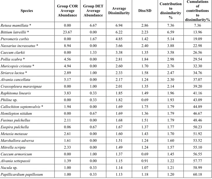
4.3.9 SIMilarity PERcentage breakdown (SIMPER)

The SIMPER routine was first described by Clarke (1993). It is an exploratory analysis to locate which species are the greatest contributors to differences between sites or, on the other hand, which species contribute most to similarities within replicates from the same sites.

The average dissimilarity between all pairs of inter-group samples is broken down into separate contributions from each species δi. The average contribution of the ith species to the dissimilarities is usually contributed

by many pairs of samples. Therefore its standard deviation SD(δi) is informative too.

If is large and SD(δi) small the ratio /SD(δi) is large too, then the ith species not only contributes much to

the dissimilarity between groups 1 and 2 but it also does so consistently in inter-comparisons of all samples in the two groups. It is thus a good discriminating species.

The results of the SIMPER routine are placed in a table like the following:

Species Group COR Average Abundance Group FOP Average Abundance Average Dissimilarity Diss/SD Contribution to dissimilarity % Cumulations of contributions to dissimilarity %

Chauvetia aff brunnea 0.44 1.75 6.27 1.17* 6.94 6.94

Bittium latreillii 23.67 6.00 6.02 1.67* 6.66 13.60

Nassarius incrassatus 8.94 0.00 4.27 2.39* 4.72 18.33

Tab. 2 – Example of the results of a dissimilarity analysis between groups with the SIMPER routine

The columns contain the following data:

- “Group X Average Abundance”: average relative abundance of the species in the X biocoenosis; - “Average Dissimilarity”: average contribution of the species to dissimilarity;

- “Diss/SD”: ratio between the average contribution of the species to dissimilarity and the standard deviation of the contribution of the species to dissimilarity, if this ratio is high the species is likely to be a good discriminating one;

- “Contribution to dissimilarity %”: percentage contribution of the species to dissimilarity;

- “Cumulations of contributions to dissimilarity%”: cumulation of the percentage contribution of the species to dissimilarity.

(25)

21

In much the same way, the contribution each species makes to the average similarity within a group can be examined. The more abundant a species is within a group, the more it will contribute to the intra-group similarities. It typifies that group if it is found at a consistent abundance throughout so that the standard eviation SD(Si) is low and the ratio /SD(Si) high.

The results of the similarity analysis by the SIMPER routine are placed in a table like the following:

Species Group COR Average Abundance Average Similarity Sim/SD Contribution to similarity % Cumulations of contributions to similarity% Bittium latreillii 23.67 7.88 2.13* 16.95 16.95 Nassarius incrassatus 8.94 4.61 2.26* 9.93 26.88 Pollia scabra 4.56 3.31 2.23* 7.11 33.99

Tab. 3 – Example of the results of a similarity analysis within a group with the SIMPER routine

The columns contain the following data:

‐ “Group COR Average Abundance”: average relative abundance of the species in the X biocoenosis; ‐ “Average Similarity”: average contribution of the species to similarity within the biocenosis;

‐ “Sim/SD”: ratio between the average contribution of the species to similarity and the standard deviation of the average contribution of the species to similarity; the higher it is, the more the species is typical to the biocoenosis; however, this does not mean the species is typical only of one biocoenosis, but it can typify more than one;

‐ “Contribution to similarity”: percentage contribution of the species to similarity;

‐ Cumulations of contributions to similarity%”: cumulation of the percentage contribution of the species to similarity.

4.3.10 PERmutational Multivariate ANalysis Of VAriance (PERMANOVA)

PERMANOVA is a computer program for testing the simultaneous response of one or more variables to one or more factors in an ANOVA experimental design on the basis of any distance measure using permutation methods (Anderson, 2005). The method is described in detail in Anderson (2001) and McArdle & Anderson (2001).

PERMANOVA can be applied to the values of similarity matrices or to their ranks alike, this being a difference from ANOSIM (pag. 19) in the one-way case.

When the number of possible permutations is too low, the program uses Monte Carlo sampling to construct the asymptotic permutation distribution for the entire F statistic (Anderson et al., 2003). This helps resolving problems of level of significance higher than desired because of the small number of samples.

4.4 Biodiversity indices

Biodiversity indices were used to synthetize the information hidden in samples both using them without further computing or using them in statistical tests (e.g. analysis of variance).

The following biodiversity indices were used.

4.4.1 Number of species (S)

This index is just the total number of species present. The more species there are, the more diverse the sample.

However, this index has to be used with care since its use in non comparable samples may mislead the analysis. For example, it strictly depends on the sampling effort (the bigger the sample, the more species are likely to be).

For this reason, in this thesis it has been mainly used to compute more complex indexes, like Margalef species richness.

(26)

22

4.4.2 Number of specimens (N)

This index is not a true diversity index, but it is an abundance index.

It gives information on the quantity of specimens per sample and when used in relation to the area sampled can describe the density of living specimens in the different samples.

4.4.3 Margalef’s species richness (d)

Since the number of species is sample dependent, it is not suitable when different sampling techniques are used or when there are doubts that sampling has been carried out with the same efficacy.

Margalef’s species richness index is based on the number of species, but incorporates the total number of individuals too:

1 log Where:

S is the number of species; N is the number of specimens.

4.4.4 Shannon index (H’)

This is the most commonly used diversity index and is computed by: · log where:

is the proportion of the total count arising from the ith_species:

The higher the value of the index, the more diverse is the sample. Note that the natural logarithm is used.

The Shannon index can be sensitive to the degree of sampling effort and should be compared across equivalent sampling desings.

4.4.5 Equitability (J’)

This index expresses how evenly the individuals are distributed among the different species. It is referred as Pielou’s evenness index too. It is computed by:

log

This index is close to 1 when all species are equally abundant. It is close to 0 when the sample is highly dominated by a few species.

4.4.6 Simpson index (λ)

This is another commonly used index which has a number of forms. Here two forms are used:

1 1

where:

(27)

23

The index λ has a natural interpretation as the probability that any two individuals from the sample, chosen at random, are from the same species. λ is always ≤1.

It is a dominance index, in the sense that its largest values correspond to assemblages whose total abundance is dominated by one, or a very few, of the species present. Its complement 1- λ is thus an equitability or evennes index, taking its largest value when all species have the same abundance.

4.5 Biodiversity estimators

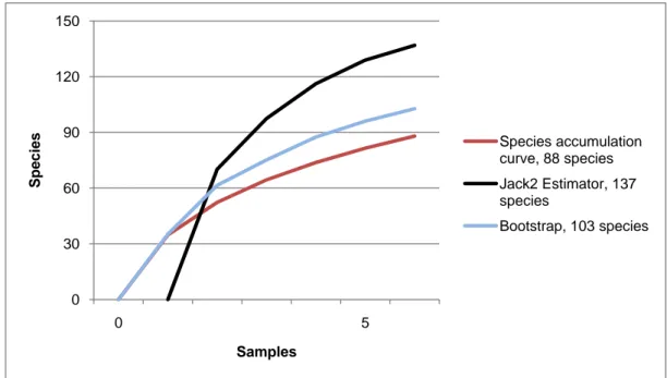
Accumulation curves were drawn with EstimateS 8 (Colwell, 2006) with 50 randomizations. Biodiversity estimations were done using the Bootstrap non-parametric first order estimator (Smith et al., 1984) and the Jackknife non-parametric second order estimator (Burnham et al., 1979). The first order estimators take into consideration singletons only, while the second order estimators take into consideration doubletons too. Singletons are defined by Novotny & Basset (2000) as species represented by a single specimen in the sample. Doubletons are those represented by two specimens in the sample. Species found as a single individual in component communities are called “local singletons”, those found as a single individual in the combined data set are called “unique singletons”.

4.6 Trophic groups and feeding guilds

Trophic information for all species was mined from the literature. A great effort in citations was placed for every species, the reference is given as a foot note. The following priorities were followed:

1. Specific literature about the species;

2. Specific literature about species of the same genus within the same biogeographic province;

3. Specific literature about species of the same genus or systematically closely related outside the biogeographic province;

4. General references on the supra-specific group.

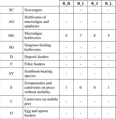
It has been decided (arbitrarily) to use the same classification of feeding modes and guilds used by Rueda et

al. (2009) (Tab. 4) for the sole reason that it allows comparison with a work with a similar approach but on a

different biocoenosis (Zostera marina beds) in a different geographical area (Alboran Sea).

Code Feeding guild description Examples

SC Scavengers Nassariidae

AG Herbivores of macroalgae and epiphytes Williamia

MG Microalgae herbivores Most Trochidae, Cerithiidae, Rissoidae SG Seagrass-feeding herbivores Smaragdia

D Deposit feeders Nucula, Nuculana, Tellinidae, Semelidae

F Filter feeders Most bivalves, with the exception of _{deposit feeders} SY Symbiont-bearing species A few bivalves (Solemya, Lucinidae, _{Thyasiridae, Xylophaga)}

E Ectoparasites and carnivores on preys without _mobility

Triphoridae, Cerithiopsidae, Eulimidae, Epitoniidae, Coralliophilinae,

Pyramidellidae, some opisthobranchs C Carnivores on mobile prey Turridae, most Muricidae, some _{opisthobranchs} O Egg and spawn feeders Mitrella minor

(28)

24

4.7 The role of species in describing biocoenoses

When describing the fauna of biocoenoses, species can be ascribed to three different categories:

‐ Characteristic species: these species are typical of a biocenosis, meaning that they are usually found in it notwithstanding their abundance which can be high (constant species) or low (sporadical species). This group can be divided in two further groups: the exclusive species which can be found only in a given biotope or the species which prefer the biocoenosis, meaning that in that biotope they are significantly more abundant than in others.

‐ Accompanying species: these species are normally present in the given biocoenosis as in others. These species may appear at the given depth level, or can be indicators of edaphic conditions or may have wide ecological tolerance and are usually ubiquitarian.

‐ Accidental species: these are species characteristic of other biocoenoses but occasionally found in the given biotope where they experience limited success (reduced life span, increased predation, inability to reproduce,…).

Particular attention should be given in classifying species which are parasites, symbiontic, commensals or are species-specific epibiontic. Their attitude towards biocoenoses will depend by their host and not by themselves, of course.

Another issue to be considered in general, but which is probably of low interest in benthic molluscs, is that some species may have a different affiliation to biocoenoses in different stages of their development.