Distance to default and the ability of KMV model to forecast default

U

NIVERSITY

OF

P

ISA

"

D

EPARTMENT

OF

E

CONOMICS

AND

M

ANAGEMENT

M

ASTER

IN

C

ORPORATE

F

INANCE

AND

F

INANCIAL

M

"

"

Distance to Default and the ability of

KMV model to forecast default

"

"

"

"

SUPERVISOR

!

Prof.ssa Sara Biagini

CANDIDATE

Agnese Bonadio

"

"

Acknowledgments

"

"

First, I would like to express my gratitude to my supervisor for her support, patience and guidance.

I do appreciate her professional instructions, recommendations and useful comments. Thanks to the University of Pisa who allowed me to spend a period of study abroad, in UK. So far, that one was the most incredible, exciting, challenging experience of my life. I would go back to study just for that reason. No joke…

Thanks to all my friends, those I see only few weeks a year, those I see every day, those who suffer and struggle with me while riding a bike.

Thanks to all my family. Each of them, in some way, make me feel like I am not alone. A special word of thanks to my brother, who helped and supported me writing the Matlab codes and needless to say supported and “stand me” during these years.

Thanks to my boyfriend, who has the hard ”job” of making me happy every day.

"

Finally, no words would be enough to express deep gratitude and infinite respect to my parents: they have supported, trusted and loved me every single day and always they will.

"

"

"

"

All errors are the responsibility of the author.

"

"

""

"

Contents

"

Introduction

9

Credit risk and default event ...10

1. Merton Model

13

1.1 Default forecasting model ...13

1.1.1 Structural approach ...13

1.1.2 Reduced-form approach ...16

1.1.3 Incomplete information approach ...17

1.2 Literature review ...18

1.3 Merton Model ...20

1.3.1 The theoretical framework ...20

1.3.2 Assumptions ...20

1.3.3 Basic idea of Merton ...23

1.3.4 Calculation of Distance to Default measure ...27

1.3.5 Limits of Merton’s model ...31

1.3.6 Beyond the Merton model ...32

2. MKMV Model

35

2.1 General background ...35

2.2 MKMV model assumptions ...37

2.3 Characteristics of MKMV model ...39

2.4 Main steps ...39

2.4.1 Identification of the default point ...39

2.4.2 Estimation of asset value and volatility of asset ...40

2.4.3 Calculation of Distance-to-Default measure ...43

2.4.3.1 General considerations on DD

...

43

2.4.4 Calculation of the Expected Default Frequency ...45

2.4.4.1 EDF vs. agency rating

...

49

2.6 Financial and economic factors that influence DD ...53

2.7 Strength ...55

2.8 Weaknesses ...56

2.9 Merton-MKMV comparison ...56

2.10 Final remarks on MKMV model ...57

3. Methodology

59

3.1 Parameters setting ...59

3.1.1 Observable parameters ...59

3.1.2 Unobservable parameters ...63

3.2 Distance to default calculation ...64

3.2.1 Distance to capital for financial firms ...65

3.3 Probability of Default calculation ...65

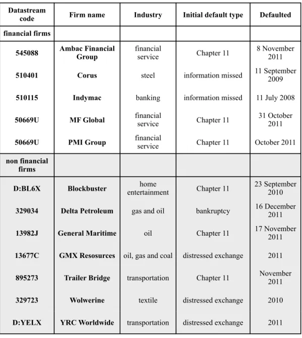
3.4 Sample selection ...65

4. Results and analysis

71

4.1 USA defaulted firms ...71

4.2 EU defaulted firms ...75

4.3 USA not defaulted firms ...78

4.4 EU not defaulted firms ...81

4.5 Further considerations ...84

Conclusion

91

List of tables: summary statistics

95

Appendix A: Volatility Estimation

121

Appendix B: Matlab codes

123

Introduction

"

The latest financial crisis has traumatized the global financial markets.

The causes of the crisis are complex and multiple and credit risk management has played a decisive role in the events that triggered this crisis. Therefore, in the recent years, new techniques and new methods for measuring credit risk have been developed.

In order to stay competitive, to raise capital for growth opportunities, “to reduce the chance of default and the cost of financial distress” (Smith and Stulz, 1985), agencies banks and firms are trying to apply and enforce these methods in innovative ways. Besides, the crisis has shown how having a good credit rating is not a guarantee of good financial health of a firm. It is therefore questionable how effectively ratings are formulated and if credit models are truly reliable.

The need to develop new systems for the risk measurement is then due to:

-

-

-

-

-

-

"

Nevertheless several models have been developed for hedging out the default risk, these models are not sufficiently adequate to deal with the complex and confused uncertain randomness of financial markets. For example, most approaches rely on the market efficient hypothesis (EMH), according to which all information should be incorporated into the prices. But it has been repeatedly demonstrated that the strong

form of EMH does not hold in the real world: markets are not efficient neither well informed . 1

The full understanding of credit risk models, such as Merton’s and MKMV’s, preliminarily requires both the definition of insolvency and then a quick analysis of the theoretical context in which the model itself was developed.

Let’s start giving a definition of credit risk (also named default risk) and then move within this to examine the Merton approach on the determination of the probability of default according to the principle of contingent claim analysis from which the model is inspired.

"

Credit risk and default event

Risk, by definition, is a situation involving exposure to danger, possibility of financial loss.

Credit risk refers to the risk that a firm does not meet its debts on time. Basel Committee defines credit risk as “the risk that a borrower will default on any type of debt by failing to make required payments ”. 2

Usually, default of a firm is associated with its bankruptcy, a legal term that exhibits inability to pay own debts. However, default is different from bankruptcy: the latter is when the firm is liquidated, the former is an event in which the firm cannot meet its financial obligation. For example, a firm could have a financial situation that makes it insolvent at a particular time, but may not be at the time in which it is declared insolvent from rating agencies.

This variety of notions above described is in agreement with Moody’s definition: they assert that corporate default is triggered by one of these three events:

1. a bankruptcy filing

“The market does not reflect accurately all the information in the financial statements”, Sloan, 1996.

1

Principles for the Management of Credit Risk, Final document, Basel Committee on Banking

2

2. a distressed exchange where old debt is exchanged for new debt that represents smaller obligation for the borrower

3. a missed or delayed interest or principal payment

Finally, there is another “empirical” definition, according to structural models: straightforwardly, default occurs when the value of the assets is smaller than a barrier, identified as the default point. The crucial matter is the estimation of this barrier, which may be deterministic or stochastic.

From now on, we identify default as described just above: when the value of assets is smaller than the default point, a firm will default.

"

Once it is clear what we mean by default event, it can be easily understood the impossibility of establishing a priori whether a company will default or not at a certain date in the future, since we not may know in advance whether it will be able to meet its debt or not.

Forecasting is predicting future using the information we have today, at present day. The decisions we make today, will affect the future events. Ultimately, default events are unpredictable and costly and the best we can do it is to calculate the probability these events will happen.

"

In this thesis, structural models are described, with particular attention to Merton model and its implementations and a new indicator, the distance to default ratio, is illustrated. The main purpose of this work is then to investigate if this new measure of default risk is a good indicator of financial distress as well as if it has any forecasting power.

"

The structure of this thesis is organized as follows: Chapter 1 describes the Merton model and the notion of the distance to default ratio, after a quick introduction to default forecasting models; Chapter 2 focuses on the MKMV model, one of the modern credit risk qualitative measuring models, its methodology and the expected

default frequency (EDF); Chapter 3 describes the methodology we used in our analysis, the parameters estimation as well as a description of the data sample; in Chapter 4 we present and discuss our results.

The last part contains summary statistics of the most important inputs/outputs of the models, followed by conclusions.

Besides, two appendices concerning volatility calculation and the Matlab codes are provided at the end of this work.


1. Merton Model

1. Merton Model

"

"

1.1 Default forecasting model

"

At present, in the finance literature, there are three different approaches for estimating credit risk: the structural approach, the reduced-form approach and the incomplete information approach. Each approach uses different methods and relies on different assumptions.

Despite of the existence of several and different methods of managing credit risk, measuring credit risk is not an easy task since data used by agencies and credit risk modelers are confidential and not available publicly.

Below in details the different approaches above mentioned.

"

"

1.1.1 Structural approach

"

Also known as contingent claim approach or option pricing approach, the structural model is so called because the default probability is based on the liability structure of a firm and credit risk is driven by the firm value process. For this reason, these models are also known as “firm-value” models.

“Structural model means it has the characteristics of describing the internal debt

structure of a company where default is a consequence of an internal event”. 3

The main purpose of these approaches is to provide a relationship between default risk and the capital structure of the firm.

The structural model is very simple in its idea. If the firm’s asset value (V) is below the default point (DP), we can predict the firm default. However, prior the default event,

Saunders, A. & Allen, L., 2002, Credit Risk Measurement: New Approaches to Value at Risk and

3

1. Merton Model there is no way to discriminate between risky firms and stable firms. Indeed the complexity comes up when trying to predict default into the future, at the end of the period considered. A good predicting model would avoid additional costs and gain a better portfolio performance. For example, banks usually use default prediction models for loans applications and capital allocation purposes.

In structural models, default is seen as an exogenous event, which depends on the behavior of the firm’s value during a specified period of time. The idea of applying the option pricing theory to the problem of bond valuation and other credit risk exposures goes back to the intuition of Merton in 1974: the firm’s equity value is simply a European call option on the asset value V and default can only happen at maturity T. Examples of structural models are: Merton model, Black and Cox model (1976), KMV model.

"

In the Merton model, assumptions are made on the dynamics of the firm’s assets value, on its capital structure and on its debt. The firm’s asset value V is assumed to follow a Geometric Brownian Motion, the capital structure is relatively simple and it supposes the firm has just one zero coupon debt issue.

Simply, a firm defaults when V is below some threshold (the default boundary), interpreted as a liability.

However, these assumptions given above, imply many important consequences and also represent at the same time the two most obvious limitations of the study conducted by Merton. Firstly and perhaps most importantly, considering the debt structure of the firm as a zero coupon bond implies that a firm’s default may occur only at maturity (when the face value of the debt F is higher than the asset value V). Secondly, the assumption on the dynamic of V leads to the fact that the probability of default is predictable in relation to the given time horizon, since it is predictable the evolution of V (advantages and disadvantages of Merton’s model are described in the next paragraph).

1. Merton Model Such limits are the main reason that led to the subsequent generalizations of the Merton model. Among them, we first recall Black and Cox (1976).

Their study is important mainly due to the fact that considers the possibility that default can occur even before T, if the assets value drops below a certain level: in other words, default can occur at any time.

However, the assumptions on V are the same as Merton’s.

A similar approach to those just stated is the Credit Monitor Model developed by KMV Corporation. Default occurs when the assets value is below the default point, which is somewhere between short-term liabilities and long-term liabilities.

"

The main advantage of the structural approaches is that they are simple to understand and they provide a very intuitive picture as well as an endogenous explanation of the default event (this means that the default event is derived from the model).

Disadvantages can be identified in its difficulty of implementation analytically and computationally . Furthermore, since structural models depend on the firm’s asset 4 value (V) and on the volatility of the firm (! ) and neither is directly observable, a clear difficulty is their calibration. Another shortcoming is that the basic assumptions are unrealistic, they do not reflect the reality of financial markets. In the end, if the capital structure of the firm is complicated (and asset prices are not easily observable as they assume), these questionable assumptions fail and these models cannot be used. Lastly, most structural models assume complete information in order to give a better explanation of a firm performance (but this is a very oversimplified hypothesis).

Structural approaches assume that practitioners have the same information of firm’s manager whereas reduced-form models assume they only have the information incorporated into the market, regardless of the knowledge of liabilities value and asset value of the firm.

"

"

σ

“Structural models are also computationally burdensome”, Bo Liu, A. E. Kocagil, G. M. Gupton,

4

1. Merton Model

1.1.2 Reduced-form approach

"

The reduced-form approach is a relatively recent method of estimating credit risk, where default is considered as an exogenous “unexpected” event, not linked to the capital structure of the firm.

This kind of perspective is more general. Unlikely the structural approach, it does not assume any particular model of the firm’s liability structure. This method considers default as an exogenous event (refers to assumptions specified outside the model) and considers default as a random variable driven by a stochastic process (typically assumes a Poisson’s process). Default may happen at any point in time, there is no explanation in terms of fundamental quantities and firm’s default time is unpredictable.

The reduced-form models are characterized by flexibility: this is a strength and a weakness at the same time. They are entirely data driven and generally produce better results for credit risk pricing than structural models.

Example of reduced-form models are CreditMetrics (also known as RiskMetrics) and ! . The former, based on an insurance approach, models default as a continuous variable with an underlying probability distribution. The main disadvantage of this approach is that all firms within the same rating class have the same default rate which is equal to the historical average default rate (since probabilities are calculated on the average historical frequency of defaults).

In the latter, default happens as a surprise (at any point in time), since the default event is exogenous. ! is easy to implement and very attractive from a computational point of view but it ignores the migration risk (the probability and value impact of changes in default probability ) and the market risk since interest rates are 5 assumed to be deterministic.

In these kind of approaches default time is modeled so as to be independent from the underlying securities or from interest rates.

CreditRisk+

CreditRisk+

Definition from Modeling Default Risk, P. Crosbie and J. Bohn, Moody’s KMV, December 2003.

1. Merton Model

1.1.3 Incomplete information approach

"

It is a combination of the two above mentioned approaches, it is a kind of hybrid model.

An example of incomplete information approach is CreditRatings: rating agencies collect information from the market and from financial statements in order to “evaluate” companies and assign them a rating class (credit quality) from AAA to D. After that, default probabilities are estimated for each group and all firms with the same rating category have the same probability of default. This methodology allows the efficient use of information and allows financial institution to estimate the default probabilities of all their clients. However, there are some aspects of this method that investors do not like, such as the fact that agencies do not change so often the ratings of a company (ratings are adjusted in a discrete fashion whereas default rates evolve continuously) and these judgments are not always reliable (the recent financial crisis is such a proof ). 6

"

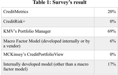
Clearly, all modeling framework have their own set of advantages and disadvantages. In a survey , conducted in 2002, a number of firms were asked whether they were 7

using a portfolio model and which model. About 85% of the respondents indicated that they were using a credit portfolio model.

The table below summarizes the responses : 8

"

"

Emblematic was the case of Lehman Brothers, a global financial service firm: in 2007 it was ranked

6

the #1 “Most Admired Security Firm” by Fortune Magazine; in 2008, on the 18th of July its stocks seemed to have high reliability as confirmed by the most famous rating’s agencies: A by

Standard&Poor’s, A2 by Moody’s, A+ by FitchRatings. Two months later, on the September 15, the company declared bankruptcy.

Smithson, Survey of Credit Portfolio Management Practices, 2002.

7

These responses sum to more than 100%, because some respondents checked more than one model.

1. Merton Model

"

"

1.2 Literature review

"

Lots of researchers have examined the contribution of the Merton model over the past years. A question still open for discussion among academics is which modeling approach has a better forecast power.

There is not an absolute answer to that questions. Many factors should be taken into account and an empirical evaluation is strictly necessary in order to test each model and identify strength and weakness of each method in measuring credit risk.

Arora, Boh, Zhu (2005) tested structural models (Merton and Vasicek-Kealhofer model) and reduced-form model (Hull-White model) to understand if they have any predictive power and which approach is better in discriminating defaulting firms from non-defaulting firms. They found that VK and HW models outperform the Merton model. Moreover, they point out that Merton’s is not good enough to discriminate defaulting and non-defaulting firms.

Jarrow, Lando and Turnbull (1995) and Hull and White (2000) presented detailed explanations of several reduced-form approaches.

Table 1: Survey’s result

CreditMetrics 20%

CreditRisk+ 0%

KMV’s Portfolio Manager 69%

Macro Factor Model (developed internally or by

a vendor) 6%

MCKinsey’s CreditPortfolioView 0% Internally developed model (other than a macro

1. Merton Model Hilscher, Jarrow and van Deventer said that “the reduced-form approach can never be 9 less accurate then the Merton approach”. Indeed they believe the reduced-form approach has a better predictive power as well as a better forecasting ability.

Bharath and Shumway (2005) showed that the reduced-form approach has a better predictive power in the U.S. corporate defaults. In particular, they examined the accuracy of default forecasting and how realistic its assumptions are. In order to exceed the limits of Merton’s, they suggested a model with a näive alternative, with better predictive power (as they stated). They concluded saying that the Merton DD probability has some predictive power; however they asserted that “[…] most of the marginal benefit comes from its functional form rather than from the solution of the Merton model ”. 10

Crosbie and Bohn (2003) described the KMV model as an implementation of the Vasicek-Kealhofer model and pointed out the effectiveness of KMV models in dealing with credit default (after making some modifications on the assumptions).

Black and Cox (1976) modeled the default point as an absorbing barrier and support the reduced-form models.

Duffie, Saita and Wang (2007) said that the Merton DD ratio has a “significant predictive power”.

Duan (1994) proposed another method of estimating asset value and asset volatility, based on maximum likelihood estimation using equity prices.

In 2004, the new Basel Capital Accord also recommended the IRB (Internal Rating Based Approach) to control credit risk.

"

It is clear that there is a lot of uncertainty to which is the best model for estimating credit risk; however it is important to realize that the need to have this kind of

J. Hilsher, R. A. Jarrow, D.R. van Deventer, Measuring the Risk: A Modern Approach, July-August

9

2008, The RMA Journal.

S. T. Bharath, T. Shumway, Forecasting Default with the Merton Distance to Default Model, Oxford

10

1. Merton Model instruments, in order to measure manage and narrow credit risk, is becoming crucial in the financial markets.

"

"

1.3 Merton Model

"

1.3.1 The theoretical framework

"

The Merton model is an extension of Black & Scholes model (1973) on option pricing theory. It is a structural model and it looks at the evolution of the capital structure of the firm to evaluate its credit risk.

Merton gives a powerful intuition about corporate default and helps understand which factors affect the default probability. Moreover he provides important understanding in the valuation of equity and debt, when the probability of default is not trivial to calculate.

This approach requires perfect observability of the balance sheets (asset value and debt value in particular), however the last financial crisis showed that balance sheets are terribly opaque and not all data are publicly available.

"

"

1.3.2 Assumptions

"

The model’s assumptions are:

"

frictionless market


there are no transaction costs, no taxes, no bankruptcy costs, continuos time trading, unrestricted borrowing and lending at a constant interest risk-free rate, complete information, infinite divisibility of assets, short-selling is allowed;

1. Merton Model market perfection


operators are price takers, agents prefer more wealth to less wealth, perfectly competitive market;

"

debt


the model does not distinguish between different types of debts, it supposes the firm has just one zero coupon debt issue D, with face value F, maturing in T periods. The 11 firm agrees/settles to pay the bond to the bondholder at maturity.


It is clear that this is a critical assumption: here the default can occur only at the maturity of the bond.


"

capital structure


the balance sheet of the company is in a particularly simple form and it looks like:

(source: Moody’s )

"

From the accounting identity we have:

! (1) where V is the firm’s total asset value, E is the equity (pays no dividend) and D is the market value of debt . 12

"

Table 2: Merton’s balance sheet

Assets Liabilities firm value: V(T) debt: D(V,T)

equity: E(V,T)

total V(T) V(T)

V(T)= E(V,T)+ D(V,T)

“Face value is commonly referred to the amount paid to a bondholder at the maturity date, given the

11

issuer does not default”, Investopedia.

The market value of the debt is the price at which buyers and sellers negoziate debt-purchase

12

agreements. Estimating the market value of debt is not simple since very few firms have all their debt in the form of bonds. One way to estimate it is by converting this debt into a hypothetical coupon bond with face value F.

1. Merton Model The intuition is simple and straightforward: the value V(T) of a company is seen as the market value of all assets (tangible and intangible). Assets are purchased with the money of shareholders through the capitalization of the equity E or through the debt D (in other words, the firm is financed with debt and equity, all debt expires at time T, the debt is fixed and the future asset value V(T) is uncertain). Firm's assets are first used to pay debtholders and, whatever is left, it is distributed to shareholders.

"

dynamic on V(T)


For simplicity, this method considers V as a stochastic process, in particular it assumes

V is log normally distributed with constant volatility.


The model assumes that V(T) follows a Geometric Brownian Motion (GBM) . That 13 means:

! (2) where ! is the instantaneous constant expected rate of return, ! is the constant volatility of the asset’s return on the underlying asset (it is assumed to be constant) and ! is a Wiener process.

"

Parameters relevant to the model are:

"

V is the market value of the assets of a company which is the present value of all

future cash flows produced by the company;

F is the amount of the liabilities of a company based on the value at which they are

recorded in the financial statements; in practice it is the amount that the firm is required to pay its creditors;

! is the asset risk, the results in the return volatility of the market value of the assets; it measures the level of uncertainty.

dV_T V_T =µVdT +σVdWT µ_V σV WT

σ

This assumption is very important, since it implies that the instantaneous log returns are normally

13

distributed with constant variance and they are independent. The GBM model is a reasonable model of stock price movements.

1. Merton Model It is easy to see how the variables listed above actually enclose all the elements necessary for the determination of the probability of default of a company: V includes the future expansion and evolution of a company as well as the economic sector to which it belongs; ! (the ratio between the total liabilities and the total asset) expresses the financial risk; eventually, the degree of business risk of the company is implicitly considered in ! .

Among these three variables, only F is known. V and ! are not directly observable.

"

Under these assumptions, default happens when asset value is below the face value of the debt F: default is not allowed before maturity time.

"

"

1.3.3 Basic idea of Merton

"

The basic idea of Merton is about the option nature of the equity: the model considers the firm’s equity as a call option on its assets. Conceptually, we have a firm that is continuously borrowing and retiring debt and we have two types of agents: equityholders (those holding shares of the firm’s equity) and debtholders (those owning bonds); generally, equityholders has the right to receive a portion of the firm’s profit in the form of dividends and may have the control of the firm; debtholders have the right to receive principal and interest on the debt and, in the event of bankruptcy, they have the priority over equityholders in the liquidation of assets. Bondholders could be viewed as holding a short put position on the firm’s assets. On the other hand equityholders can be seen as holding a call option on the asset value of the firm. At maturity time T, when the debt matures, debtholders are repaid the face value F of their bonds.

At this point, there are two possibilities: the value of assets exceeds the value of the debt or not. In other words, if V(T)>F, then debtholders receive F and shareholders

F V

σV

1. Merton Model receive the residual value V(T)-F=S(T) and there is no default. Otherwise, if V(T)<F, then the firm cannot meet its financial obligations and shareholders hand over control to the bondholders, who liquidate the firm. So, default occurs, debtholders only receive the value of assets V(T) and equityholders have 0. For that reason, at time T, debtholders have the right to receive min(F, V(T)), whereas equityholders have

max(V(T)-F;0): that is the payoff of a call option on V with strike price F.

This is the intuition behind the model: the value of equity is equivalent to a European call option on the underlying asset value V with strike price F maturing at T.

"

The payoff of a European call option with these characteristics is shown in the figure below:

The result of the Merton model is summed up in the following equation, according with the option pricing theory:

! (3) where ! (4) ! (5) E₀=V₀N(d₁)- Fe-rT N(d₂) d 1= lnV0 F + r + σ_V2 2 ⎛ ⎝ ⎜ ⎜ ⎞ ⎠ ⎟ ⎟T σ_V T d₂= d₁-σV T M arke t va lue of e qui ty E

Face value of debt F

0 10 20 30

1. Merton Model and ! is the cumulative standard normal distribution function and r is the risk-free rate.

The formula (3) holds for every successive time t<T.

"

Thereby, bearing in mind that the price of an option is a function of five variables (exercise price, the market value of the underlying asset, time to maturity, interest rate, volatility of the underlying asset), it can be set the following relation:

!

It expresses the value of a firm’s equity as a function of the value of the firm.

Further, by Ito’s lemma, the stochastic differential equation defining the dynamic of E is given as:

! (6) Since V follows a GBM, we can subsisted the following expression in (6):

!

and obtain:

!

We then have the following terms:

"

"

( )

( )

(

)

(

)

1. Merton Model

!

The volatility of the firms asset value ! is then related to the volatility of the firm’s equity ! as shown below:

! (7) Under the B&S formula it can be shown that ! is the equity delta of a call:

!

We can now write down the theoretical link between the volatility of the market value of the equity (which in turn can be represented by the volatility of the stock price ! ) and the volatility of the firm:

! (7-bis)

"

In most application of B&S, strike price (F), time-to-maturity (T), underlying asset price (V), risk-free rate (r) are easily observable and only volatility (! ) need to be estimated. In Merton, conversely, the value of the underlying asset (V) is not observable whereas the value of an option is observed as being the total value of the firm’s equity (E). Therefore ! can be estimated but ! must be inferred.

"

From the above results, a system of two nonlinear equations must be solved:

! (8)

All the variables are known (E, F, r, T are observable, ! is estimated). µEE = 1 2EσVV 2 + E + EVµV ⎛ ⎝⎜ ⎞⎠⎟ σEE =

(

)

σ

σ

σ

σ

σ

σ

σ

1. Merton Model However, as we have already said, the firm value V is not observable, which makes assigning values to it and its volatility ! problematic.

"

Before calculating the probability of default of a firm, once V and ! are inferred by solving the system, the distance to default is defined as:

! (9) The distance to default (from now on DD) is the amount of standard deviations the asset value is far from default. The term µ that appears in the formula given above is the drift rate. Drift estimation is quite difficult (see next paragraph for more details).

"

"

1.3.4 Calculation of Distance to Default measure

"

The distance to default is expressed as the number of standard deviations the firm’s asset value has to drop before default occurs. The large the number of standard deviations, the smaller is the default probability of a company.

Statistically it can be interpreted as by how many standard deviations move in the asset’s value will the firm default.

The DD formula (assuming a lognormal distribution for V) is as defined in (9).

"

Let’s explain the formula:

the numerator is giving an expected continuous return above the threshold by combining two pieces:

! is the implied return already in the capital structure (can be seen as the distance to default at present time); it is the actual continuously compounded return on the assets that is necessary to lead to default;

σ

σ

( )

1. Merton Model the expected (geometric) return (the expected growth), µ, is the expected value of the continuously compounded return (usually positive);


! is the expected return over the whole period covered by the data measured with continuos compounding (or daily compounding, which is almost the same).

The numerator is the “surprise” or the unexpected component of the rate of return necessary for default.

The denominator is the volatility, the standard deviation of the rate of return.

We divide the numerator by the denominator just to standardize, to convert the DD ratio into normal standard units.

"

Once DD is calculated, we need to estimate the default probability (PD).

The probability of default is the probability that the asset value will be lower than the default point . In other words, 14

! (10) The value of the firm’s asset value can be expressed as (since V follows a GBM):

! (11) with µ the expected return on firm’s asset and 15 the random component of the firm’s return.

Crosbie and Bohn, by combining the equation (10) e (11), obtain:

!

"

"

[

]

[

]

From now on, the default point (DP)is identified as the face value of the debt F.

14

As in B&S assumptions, epsilon is normal distributed with an expected return equal to zero and a

15

1. Merton Model

"

!

! is normally distributed with mean zero ad variance equals to 1, so that we can express the probability of default in terms of the cumulative normal distribution:

! (12)

The probability (under the P-measure ) that a European call option at maturity is out 16 of the money is then given by the formula just described above. We therefore need to estimate µ (this is not an easy task).

Smithson says: “Credit manager does not make any assumptions about asset growth. 17 As we will see, this approach calibrates the default and migration threshold to the default and migration probabilities; so, the rate of growth is irrelevant”.

Crouhy, Galai and Mark define µ as the expected return on assets, net of out cash 18 flows.

Hurd suggests that “one possibility is to use a unique µ per sector or industry (which 19 would be easier to estimate)”.

Duffie et al. (2007), Vassalou and Xing (2004), Crosbie and Bohn (2003), Harada and Ito (2008) estimate µ and use the value in the calculation of the DD.

PD = P -ln V0 DP_T + µ -σV2 2 ⎛ ⎝⎜ ⎞ ⎠⎟T σV T ≥ε ⎡ ⎣ ⎢ ⎢ ⎢ ⎢ ⎤ ⎦ ⎥ ⎥ ⎥ ⎥ ε PD = N -ln V0 DP_T+ µ -σ_V2 2 ⎛ ⎝⎜ ⎞ ⎠⎟T σ_V T ⎡ ⎣ ⎢ ⎢ ⎢ ⎢ ⎢ ⎤ ⎦ ⎥ ⎥ ⎥ ⎥ ⎥ = N(-DD_µ)

P is the actual/real world probability, the historical or physical probability measure. When we try to

16

make a prediction, we use P.

C. W. Smithson, Credit Portfolio Management, John Wiley & Sons Inc., 2003, pag. 162.

17

M. Crouhy, D. Galai and R. Mark, Risk Management, McGraw-Hill, 2001, pag. 364.

18

M. R. Grasselli and T. R. Hurd, Credit Risk Modeling, Dep. of Mathematics and Statistics,

19

1. Merton Model Gropp. Vesala and Vulpes (2006), Nakashima and Soma (2008) use the risk free rate r instead of µ. This methodology obviously needs less data but it amounts to computing the risk neutral DD.

"

Regarding equity as a call option, present value pricing of the derivative instrument justifies the use of risk free rate. But ! is not pricing, it is future distribution estimation, requiring “real world” asset drift: this justifies the using of µ in the formula. The formula (12) gives us the risk neutral default probability (under the P-measure).

Therefore, the probability (under the Q-measure ) that a European call at maturity is 20 out of the money is obtained by replacing the drift µ with r and is given by:

! (13)

Empirically ! that means that the true physical default probability (! ) is lower than the risk neutral probability (! ).

So the Gropp. Vesala and Vulpes approach overestimates PD.

"

In the picture below, it is possible understand better this risk measure:

PD = N(-DD) PDQ_{= N} -ln V0 DPT + r -σV2 2 ⎛ ⎝⎜ ⎞ ⎠⎟T σV T ⎡ ⎣ ⎢ ⎢ ⎢ ⎢ ⎤ ⎦ ⎥ ⎥ ⎥ ⎥ = N(-DDrf ) r <µ DD_µ DDrf

Q is the risk neutral probability. It is used only for pricing.

20

1. Merton Model

!

(source: Crosbie and Bohn, 2007)

"

In the red circle, we simply ask: what’s the probability we could end up here, in this tail? This is the EDF, the expected default probability (see paragraph 2.4.4).

If V follows a normal distribution (as we assume), as a consequence the cumulative distribution is a function that tells that the probability of ending up in this tail is DD standard deviations. It’s then just a statistic.

"

However, in reality, the distribution of assets return is leptokurtic and the actual tail may be fatter than that one that appears in the figure. By assuming the log normality of

V (this hypothesis is crucial for calculating DD), the Merton model under predicts

default by a large margin. More details in the paragraph .

"

"

1.3.5 Limits of Merton’s model

"

V and ! are not even directly observable;

default occurs only at maturity T and not before, that means default is never a surprise: may happen that the firm’s value collapses to minimal levels before the

1. Merton Model maturity of the debt “but the firm is still able to recover and meet the debt’s payment at the maturity ”; in other word, in reality may happen that a firm 21 defaults when V<F for the first time, not necessary at T;

it does not apply very well when the capital structure is not simple (in reality capital structures are more complex);

risk-free rate and volatility are constant (as in Black & Scholes model, these assumptions are questionable);

the firm has just a single issue of zero coupon bond: that is not realistic;

asymmetric information problem: equity prices may not efficiently incorporate all publicly-available information about default probability; Sloan (1996) points out that the market does not accurately reflect all of the information in the financial statements;

the model applies only on firm listed on the stock exchange; if not, how can be estimated the default probability?

it assumes all liabilities are constant: but in reality firms tend to change liabilities as they approach distress, then it turns out that the Merton PD will be less than the realized PD;

asset return distribution is normal, whereas in reality asset return distribution is fat tailed;

default point is assumed to be constant, fixed at the the face value of the debt F.
 In practice, the default point is a random variable. As a firm approach default, it tends to adjust its liabilities.

"

"

1.3.6 Beyond the Merton model

"

The strength of the Merton model is that it relies on the stock price, that maybe it is the best market data for a company.

A. Kulkarni, A. K. Mishra, J. Thakker, How good is Merton Model at Assessing Credit Risk?

21

1. Merton Model “The Merton DD model is a clever application of classic finance theory, but how well it performs in forecasting depends on how realistic its assumptions are ”. 22

Moreover “ […] if the assumptions of Merton model really hold, the Merton DD model should give very accurate default forecast”.

Empirical studies have demonstrated that this approach under predicts defaults by a large margin. In particular, the hypothesis on the normality of asset returns does not reflect what happens in reality, where the value distribution is fat-tailed and extreme events are far more likely, as highlighted in the main drawbacks of the model (paragraph 1.3.5).

Given that, it would be reasonable to ask whether the Merton model is far from realistic.

It is clear that the model requires strong assumptions on the dynamics of the firm’s asset, its debt and how its capital is structured, but at the same time its background, even if quite stylized, it is enough to understand the effects of the credit risk on a firm’s governance.

The model also help understand which factors affect the default probability. Simply, Merton asserts that the probability of default can be obtained directly applying the cumulative normal distribution transformation of -DD, or PD=N(-DD) with an important assumption: normal distribution of asset returns. However, as already mentioned, in reality this assumption is almost never fulfilled and therefore it could lead to biased estimates.

For example, to make it clear, a research from Moody’s has showed how firms with 23

DD=4 are predicted to have default rate of 0,003% under the normal distribution

assumption. Empirically, firms with DD = 4 are found to have default rate of 0,6%: it is 200 times than predicted by normality assumption.

"

S. T. Bharath and T. Shumway, Forecasting Default with the Merton Distance to Default Model, The

22

Review of Financial Studies, 2008.

Moody’s EDF™ 8.0 Model Enhancements, January 29, 2007, Moody’s KMV.

1. Merton model In order to overcome these limitations, other models have been developed and practical implementations of the Merton model are today used by financial institutions. Beyond question we can say that Merton has given the structural framework on which two of the most important credit risk models are now based: Moody’s-KMV model and Credit Risk Models (CreditMetrics). Credit Ratings agencies use the Merton model for assessing the default probability and Moody’s manage some of the above drawbacks by empirical modifications, relying upon a very large proprietary database (that improves the default prediction).

Let’s see now in details the structural KMV model.

"

"

2. MKMV Model

2. MKMV Model

"

"

2.1 General background

"

The implementation of the Merton model has received considerable commercial attention in the recent years.

In the late 1980s, the Merton model was revisited by Kealhofer and Vasicek. They extended the Black & Scholes framework to produce a default forecasting model, first known as Vasicek-Kealhofer (VK) model, later named Moody’s KMV by the three company founder Kealhofer, McQuow and Vasicek (when the KMV model was acquired in 2002 by Moody’s, one of the major rating agencies, for $210 million). Today we refer to it as Moody’s KMV or MKMV model (hereafter MKMV model). Currently MKMV is the most popular commercial model for assessing credit risk ( Table 1).

Over the years, KMV Corporation has developed a credit risk methodology, as well as an extensive database (the most relevant contribution of this model is the 24 construction of an extensive database that shows the relationship between DD and

EDF, the expected default frequency).

In the MKMV approach, each company is analyzed individually without using the rating class. Indeed, MKMV has criticized the use of such methods (i.e. CreditMetrics) underlying the fact that rating are not updated so often, whereas default probabilities changes continuously (they empirically showed that some bonds rated BBB and AA may in fact have the same probability of default ). 25

The database includes over 250.000 company years data and over 4.700 incidents of default or

24

bankruptcy.

“A firm with a BBB rating could have an EDF that was also in the AAA range, or in the B range!

25

This is an astonishing amount of confusion. Could this possibly be the case? And, if so,how?”, Uses

2. MKMV Model As said above, this model is a proprietary model and therefore not all information is publicly available. Only the MKMV’s customers have full access to the database. Bharath and Shumway said: “it would be great to have MKMV data to perform similar

test, for us is too expensive ”. 26

In order to overcome this problem (the lack of information), in this thesis, the hypothesis of normal distribution of assets return is assumed.

Similar to the Merton model, a default event happens when the value of assets falls below a certain value (the default threshold). However, the default in MKMV’s is not the same as in Merton’s: default is allowed at any time ! if the asset value V crosses the barrier DP. In addition, the former considers a firm’s capital structure more complex than the latter and it estimates more deeply the default threshold on the basis of all liabilities.

Under these assumptions, the value of the firm’s assets is assumed to be log normally distributed, i.e. the log returns on the assets are normally distributed.

"

Deserve some consideration issues regarding the following questions:

why new models have been developed? what is the contribution of MKMV? how does the MKMV model improve the Merton model?

By highlighting the Merton’s limitations, we emphasized that its assumptions are unrealistic. MKMV solves some of these limitations.

Firstly, whereas in Merton the default point was constant and equal to F (the face value redeemed at maturity), in MKMV the default point is determined empirically (therefore DP is a variable and it is not constant). Since firms adjust their liabilities, the closer they are to default, the more DP varies.

Secondly, MKMV does not use a normal distribution of assets. Instead, it assumes a proprietary algorithm based on historical default rates. In other words, it implements the Merton model using a proprietary database.

t <T

S. T. Bharath, T. Shumway, Forecasting Default with the Merton Distance to Default Model, Oxford

26

2. MKMV Model The success of the MKMV approach than other credit risk models is mainly due to two reasons:

1. Moody's has a very large database of historical DD (having a large database is crucial, since the empirical measures are reliable only in the presence of large sample);

2. it uses market data for the estimation of PD, according to its large database, obtaining better results than Merton’s.

"

In order to get it clear, let’s make an example: to extend to default, default rates change continuously with current economic and financial conditions, while rating are adjusted in a discrete fashion; firms within the same rating class have the same default rate and last but not least default is only defined in a statistical sense without explicit reference to the process which leads to default (MKMV proposed a model which relates default to the balance sheet dynamics).

However, as we have already stated, since it is a proprietary model, not all information is available publicly. Analysts consider this model a “black box” because no one, expect whose work there, can’t access the database.

"

"

2.2 MKMV model assumptions

"

debt


it is supposed to be homogeneous with time of maturity T; market perfection


same conditions as assumed in the Merton approach;

dynamic of V


V is the asset value of a firm. There can be little doubt that the asset value coincides

2. MKMV Model measure to describe “the firm’s ongoing business” and varies as market participants 27 change the balance sheets and the firm’s prospects. It is more like the value that the firm can be sold. In addition, the distribution of asset returns is stable over time and the volatility of asset returns (! ) remains relatively constant.


As in Merton, the model assumes that V follows a Geometric Brownian Motion. That means:

!

with ! constant drift rate, ! and ! Wiener process.


Given this, log asset returns follows a Normal distribution function with mean and variance described as follows:

! (14)

! (15) where:

! = mean rate of return on the assets! ! = asset volatility

liabilities


the model considers short-term liabilities, long-term liabilities, convertible debt, common equity and preferred equity;

the volatility of asset returns


the volatility of asset returns remains relatively constant;

capital structure of the firm


the capital structure is relatively simple: a firm derives value from the cash flows it is expected to generate (from the assets), liabilities are paid first (however claims are

σ

dV

=

µ

V

dt +

σ

V

dW

σ

V

=V

e

σ

“The market value is different from the book value. Financial models uses market value of assets

27

because is a good measure of the value of firm’s ongoing business and it changes as market participants revise the firm’s future prospects”, M. Crouhy, D. Galai, R. Mark.

2. MKMV Model limited to principal and interest) and equity is paid second, but it has unlimited claims on the cash flow.

"

"

2.3 Characteristics of MKMV model

"

dynamics of EDF comes mostly from the dynamics of the equity values; distance to default ratio determines the level of default risk;

ability to adjust to the credit cycle and ability to quickly reflect any deterioration/ change in credit quality;

it works best in highly efficient liquid market conditions;

this pricing model is based upon the risk neutral valuation model then the expectation is calculated using the risk neutral probabilities and not the actual probabilities. Under the risk-neutral probabilities, the expected instantaneous return on all securities is the risk-free rate r, for any horizon T.

"

"

2.4 Main steps

"

The model identifies four main steps and they are the following:

"

1. identification of the default point 2. estimation of V and !

3. calculation of DD

4. use of Moody’s database to identify the expected default frequency (EDF)

"

2.4.1 Identification of the default point

"

The default point is set equal to short-term liabilities plus half of long-term liabilities.

2. MKMV Model Using a sample of hundreds companies, Moody’s empirically found that firms generally default when V reaches a level somewhere between short-term liabilities and long-term liabilities or in other word a firm survives when the value of assets is less than the liabilities that cannot be repaid in the short-term. Thus, they set the default point as short-term liabilities plus half of long-term liabilities (it is a good approximation), calculated on the basis of short-term liabilities, long-term liabilities, convertible debt, common equity and preferred equity. Given this information:

DP=STD + 0.5LTD (16) 28

where STD = short term liabilities

LTD = long term liabilities

"

In Merton, we have seen that default event happens when the value of firm’s asset is below the default point (V<DP). The key insight of MKMV’s contribution is the fact that it is possibile not to have default even if the value of the assets has fallen to less than the total debt. This is natural: generally the current cash (short-term debt) causes default (the firm may have not enough cash to keep paying all liabilities as they come due though the total liabilities may be greater than the total assets). Therefore, default occurs when V reaches some value between short-term and long-term debt liabilities. Vassalou & Xing (2004) argue that “the interest payments of the long-term debt are parts of short-term liability. In addition, the size of the long-term debt affects the firm’s ability to roll over its short-term debt, and therefore reduce the default risk.”

"

2.4.2 Estimation of asset value and volatility of asset

"

If all liabilities were listed and marked to market daily, then the estimation of the asset value of the company would be very simple, it may be inferred by simply adding the

This is purely empirical, does not rest on any theoretical foundation. The total debt is inadequate

28

when not all of it is due to one year, as the firm may remain solvent even when the asset value of assets falls below its total liabilities. On the other side, using only the short-term debt would be wrong because, for example, there are covenants that force the firm to serve other debts when its financial situation deteriorates.

2. MKMV Model value of total equity E with the value of total debts D. On the other side, the volatility of asset would be easy to calculate as well; in fact it would be sufficient to estimate the volatility of return’s ratesfrom the time series of asset values.

However, in practice, not all debt is traded, as corporate bonds, only E is marked to market daily and hence we cannot directly observe V.

By assuming a relatively simple capital structure, composed of equity, short-term debt, long-term debt and convertible preferred shares , MKMV tries to infer V taking as 29 starting point the option pricing formula of B&S, following the identical approach of Merton.

We have already said that the probability that a firm will be default is a function of two elements: the firm’s asset value (V) and the volatility of asset returns (! ).

The equity is treated as a call option written on V, exercise price is equal to the nominal amount of debt F and the expiry time is T.

In this way it is possible to express the value of equity as a function of the assets and 30 its volatility:

!

where F is set as the default point.

Similarly, it is also possible to define the link between equity volatility (! ) and the volatility of asset returns (! ):

!

! is then a function of the firm’s asset value, the asset’s volatility, the default point, the risk-free interest rate r and T.

This relationship “holds only instantaneously. In practice the market leverage moves around far too much for that equation to provide reasonable results. Worse yet, the

σ

σ

σ

σ

Vasicek (1997), Crouhy and Galai (1994) have extended the study to more complex capital

29

structure.

Since we assume T=1, we write the system in a simplified form omitting T.

2. MKMV Model model biases the probabilities in precisely the wrong direction. Default probabilities calculated in this manner provide little discriminatory power ”. 31

On this basis, all these consideration are reflected in the following system of two equations in two unknowns that we have already had the chance to introduce earlier:

!

Solving simultaneously the system is not an easy task since the solution is not straightforward ( and depend on and 32).

The MKMV method is to solve iteratively for ! . They start with an initial ! (a first guess) equals to ! , then they solve the first equation for V given E, using their first guess of ! . Then, V is introduced in the asset volatility relationship (the second equation of the system), to infer ! , with ! computed from historical equity returns. Finally, ! is then reintroduced in the first equation and so on, until ! converges. Thus E and ! are used jointly to back out V and ! .

"

These two unknown parameters, V and ! , are influenced by many factors.

Also Crosbie and Bohn (2003) observed that ! (asset volatility) is related to the size and the nature of the firm’s business. They proved that industries with low ! tend to have large DP, industries with high ! tend to have small DP.

Once V and ! are inferred, it is possible to discover the safety margin that separates a company from its failure threshold, which is the Distance to Default ratio.

"

"

σ

σ

σ

σ

E

E + DP

σ

σ

σ

σ

σ

σ

σ

σ

σ

σ

σ

σ

P. Crosbie, J. Bohn, Modeling Default Risk, Moody’s KMV, December 2003.

31

Remember the expressions (4) and (5).

2. MKMV Model

2.4.3 Calculation of Distance-to-Default measure

"

In order to avoid complexity due to µ estimation, MKMV works on its large proprietary database and uses an alternative formula to calculate DD:

! (17) where ! is the expected future asset value and (V-DP) is the so called net market worth.

The DD is the distance between the future asset value in T years and the default 33 point; it is expressed in standard deviations of future asset returns. When the distance to default decreases, the company becomes more likely to default.

"

In outline, MKMV applies the Merton model, but abandons the PD=N(-DD) in favor of PD=historical default rate. Since DD is empirical, having a database of considerable size is highly appreciable.

"

2.4.3.1 General considerations on DD

"

It is now time to make some important observations about this new quantity.

First it is immediate to conclude that the distance to default of a company is greater the lower the volatility of the return on assets and the greater the difference between the asset value and the default point.

This measure is nothing but than a ratio, increasing in V, decreasing in DP and increasing in ! . Moreover, the longer the maturity the smaller the DD, the higher the volatility the smaller the DD.

Different levels of liabilities correspond to different business risk, hence to different default probabilities. DDKMV = V_T - DP_T V_Tσ_V VT σV

Note that this DD is calculated at a time T, not at the current time T=0.

2. MKMV Model Moody’s: “the difference in their default probabilities is thus driven by the difference

in the risks of their business, not their respective asset values or leverages”.

Secondly, it is necessary to emphasize the importance of having divided the numerator (the market net worth) for the volatility changes (! ). The net market value, by itself, does not constitute a valid indicator of the risk of insolvency as it does not take into account the effects (in terms of risk) related to factors such as size, sector, industries and geographical location of the company that are rather well reflected in the asset volatility.

Then, as we said before, the distance to default represent a universal measure of risk of default able to make homogeneous (and thus comparable to each other) companies with very different characteristics (which may belong to different countries, different industries, sizes, etc.).

“The DD measure combines three key credit issues: V, its business and industry risk

and its leverage. Moreover, the DD also incorporates, via the asset value and

volatility, the effects of industry, geography and firm size ”. 34

In short, DD is a measure of company’s financial situation: as DD increases , the company becomes less likely to default; conversely, as DD decreases, the company becomes more likely to default.

"

However DD has two major limitations:

1) computationally it is not trivial; a solution to this problem would be to use a naïve

DD measure, as in Bharath and Shumway (2008), which is much easier to

calculate and “ensures, at the same time, equivalent results in terms of default prediction accuracy ”; 35

2) it is possible to calculate the DD only for publicly traded firms (balance sheet data are available with flags and on a quarterly basis only, whereas securities prices are available on a real time basis).

V

⋅

σ

Moody’s KMV Corporation.

34

G. Bottazzi, M. Grazzi, A. Secchi, F. Tamagni, Financial and Economic Determinants of Firm

35