DOTTORATO DI RICERCA IN
Ingegneria elettronica
Ciclo XXV
Settore Concorsuale di afferenza: 09/E3 Elettronica Settore Scientifico disciplinare: ING-INF/01 Elettronica
TITOLO TESI
Ultra-low power WSNs: distributed signal processing and
dynamic resource management
Carlo Caione
Presentata da: ___________________________________________
Coordinatore Dottorato
Relatore
Contents ii
List of Figures v
List of Tables xi
1 Introduction 1
2 Wireless Sensor Networks 6
2.1 Applications of wireless sensor networks . . . 6
2.1.1 Data collection . . . 7
2.1.2 Events detection . . . 8
2.1.3 Location-tracking . . . 9
2.1.4 Hybrid networks . . . 9
2.2 The energy problem . . . 9
2.3 Battery and power supply . . . 12
2.4 Radio and communication network . . . 17
2.4.1 WSN architecture . . . 18
2.4.2 Energy consumption in radio subsystem . . . 19
2.4.3 Energy saving in wireless communications . . . 21
2.4.3.1 Low-power MAC protocols for WSNs . . . 22
2.4.3.2 Duty cycling on top of MAC protocols . . . 26
2.4.3.3 Case study: Conservative Power Scheduling . . . 28
2.5 The processing subsystem . . . 34
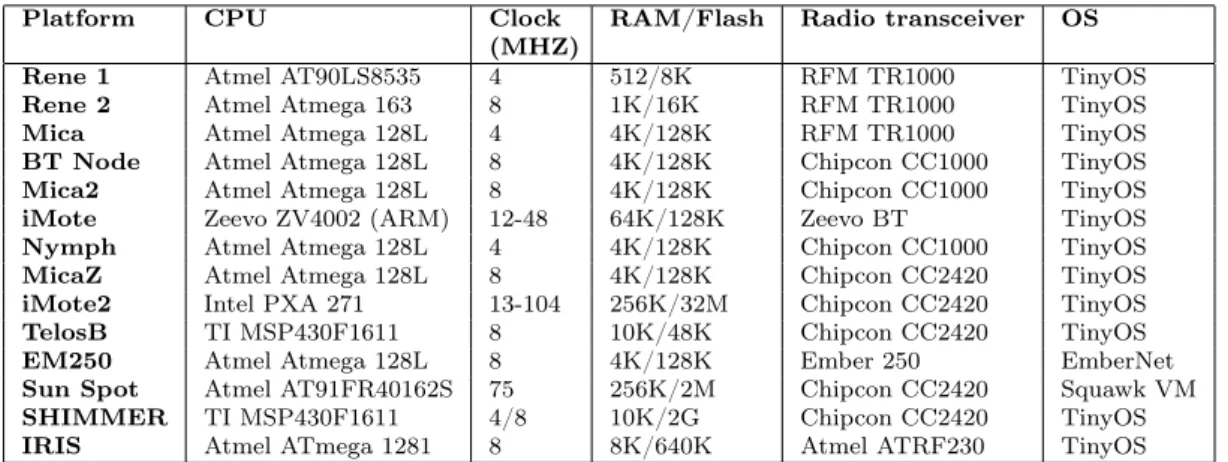
2.5.2 Sensor nodes for wireless sensor networks . . . 37
2.5.3 High-performance 32-bit micro-controllers for wireless sen-sor networks . . . 38
2.5.4 Case study: ultra-low power device for aircraft structural health monitoring . . . 40
2.5.4.1 SHM design . . . 42
2.5.4.2 Experimental verification . . . 44
3 Data reduction in WSNs 47 3.1 Middlewares . . . 48
3.1.1 Case study: SPINE2 . . . 50
3.1.1.1 SPINE2 on Ember EM250 platform . . . 52
3.1.1.2 Application scenarios . . . 56 3.2 In-network aggregation . . . 63 3.3 Compressive Sensing (CS) . . . 64 3.3.1 CS: a mathematical background . . . 65 3.3.2 Incoherent projections . . . 66 3.3.3 Signal recovery . . . 67 3.3.4 Random measurements . . . 68
3.4 Data aggregation using CS in WSNs . . . 69
3.4.1 Practical case study . . . 69
3.4.2 Data gathering and compression . . . 74
3.4.2.1 Pack and Forward (PF) . . . 74
3.4.2.2 Compressed Sensing (CS) . . . 76
3.4.2.3 Mixed algorithm: between PF and CS . . . 77
3.4.3 Mixed algorithm simulation results . . . 80
3.4.4 Energy consumption optimization . . . 84
4 Compressive Sensing for signal ensembles 92 4.1 Techniques for signal ensemble compression and reconstruction . . 93
4.1.1 Distributed Compressed Sensing (DCS) . . . 93
4.1.1.1 JSM-1 . . . 94
4.1.1.3 JSM-3 . . . 96
4.1.2 Kronecker Compressive Sensing (KCS) . . . 97
4.1.2.1 KCS for distributed sensing in WSN . . . 97
4.2 A comparison between KCS and DCS . . . 99
4.2.1 Compressibility of signal ensembles . . . 99
4.2.2 JSM-2 model for real signal ensembles . . . 103
4.2.3 Efficient DCS implementation . . . 106
4.2.4 DCS with sparse random matrices . . . 110
4.3 CS with sub-Nyquist sampling rate . . . 113
4.4 CS in embedded systems . . . 114
4.4.1 Hardware and compression . . . 114
4.4.2 Power consumption model . . . 116
4.4.3 Low-Rate CS . . . 119
4.4.4 WSN data reconstruction for Low-Rate CS . . . 121
4.4.4.1 Training data for GPSR . . . 127
4.4.4.2 Energetically optimal reconstruction . . . 128
5 Sub-sampling frameworks comparison 131 5.1 Group sparsity with CS . . . 132
5.1.1 Joint sparsity and MMV problem . . . 133
5.2 Latent variables and tensor factorization . . . 133
5.2.1 Learning process . . . 135
5.2.2 Exploiting correlations in LV . . . 135
5.2.3 Parameter learning . . . 136
5.3 Comparison between GC-CS and LV . . . 137
5.3.1 Reconstruction quality / lifetime trade-off analysis . . . 138
6 Conclusions 146
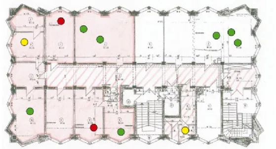
1.1 Possible deployment of ac-hoc wireless embedded network for smart-building monitoring. Sensors detect temperature, humidity and human presence at hundreds of points across the building and
com-municate their data over a multi-hop network for analysis . . . 2
2.1 Typical sensor network architecture . . . 10
2.2 Wireless sensor node power model. For each subsystem some of the major techniques for power consumption reduction are listed . 11 2.3 Ragone plot power density / power energy plot for typical energy storage technologies . . . 14
2.4 Complete power supply architecture for wireless sensor nodes . . . 15
2.5 Different WSN architectures. (a) There is no sink and the nodes communicate directly with the destination node after query. (b) Sink collects data from the sensors via multi-hop communication and forwards collected data to a remote destination . . . 18
2.6 Different collisions in WSNs. (a) Two nodes are in the transmis-sion range and send data at the same time colliding at node G. (b) Two nodes are not in transmission range but they send data approximately at the same time and again there is collision at node G . . . 21
2.7 Comparison between S-MAC and T-MAC . . . 24
2.8 A data gathering tree using D-MAC protocol . . . 24
2.9 Superframe structure for IEEE 802.15.4 protocol . . . 27
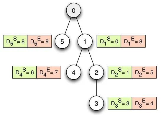
2.11 Tree-based network with associated IDs, starting and ending time slots for CPS protocol . . . 33
2.12 Scheduled network using CPS protocol . . . 34
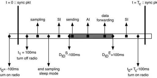
2.13 Detailed view of a communication period for practical implemen-tation of CPS protocol . . . 35
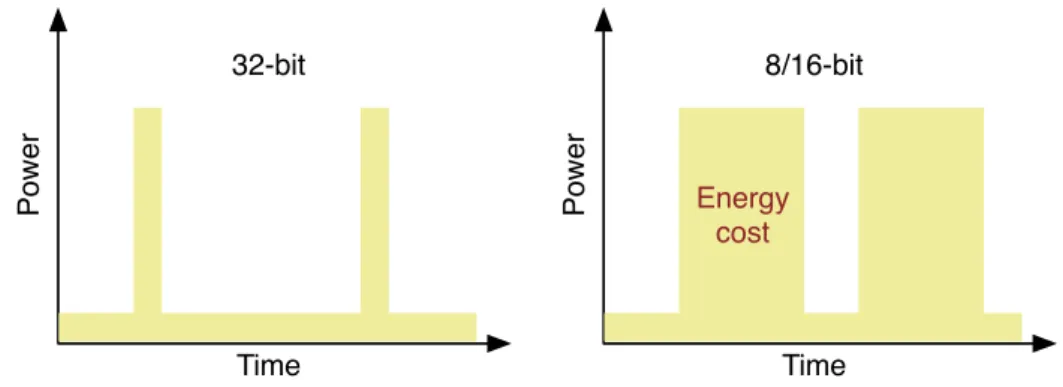
2.14 32-bit faster micro-controllers achieve tasks with less energy in comparison to old 8/16-bit micro-controllers . . . 40
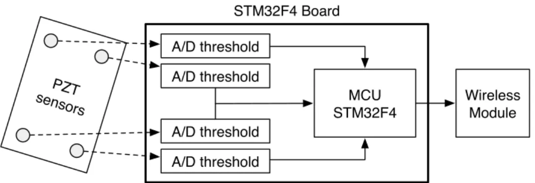
2.15 Structure of the embedded SHM device for impact detection . . . 42
2.16 Current consumption and localization error vs (a) the error itself and (b) the sampling frequency . . . 45
3.1 SPINE2 stack. The spine core separates and connects hardware and application level. The link between the core and the hardware goes through general interfaces to adapt to the specific node . . . 50
3.2 Comparison of delay in reading sensor data between SPINE2 and native Ember routines . . . 54
3.3 Delay for sending data in function of data size. Delays are mea-sured considering the time elapsed between the call of the sending routine and the callback function indicating the successful dispatch of the data packet . . . 55
3.4 SPINE2 in fall detection applications reduces energy consumption of the node. The coordinator can choose and change the evaluation function and value of thresholds . . . 58
3.5 MPC scheme using SPINE2 as underlying framework. Data elabo-ration is not performed on-node but an external controller process data coming from WSN to extract an optimal solution . . . 61
3.6 Transmission delay vs number of hops in a multi-hop ZigBee net-work when varying the traffic traversing each intermediate hops . 62
3.7 Temperature field reconstruction from LUCE deployment (March 28, 2007, 12.00AM) . . . 70
3.8 (a) Sparsity rate S function of the time of the day averaged on 10 days (NMSE=10 5) (b) NMSE for 10 reconstructed temperature
3.9 9 ⇥ 9 sensor network example adopting geographical routing . . . 74
3.10 PF and CS data aggregation techniques. Dashed rectangle is the IEEE 802.15.4 packet . . . 78
3.11 Comparison among PF, DCS, and mixed algorithm . . . 81
3.12 For network with size N > Ncrit it is clearly visible the inner zone
performing CS (black circles) and the external one composed by nodes performing PF (white circles) . . . 82
3.13 Network lifetime using Ember EM250 nodes (BID = 8bytes Bdata=
1 byte) . . . 83 3.14 (a) Lifetime of the network: comparison between PF and Mixed
Algorithm (MA) . . . 85
3.15 Lifetime extension of the modified algorithm with respect to the standard mixed algorithm vs. Bof f using network size N as
pa-rameter . . . 87
3.16 Ratio between the energy spent in compression Ecomp and energy
for data transmission and reception ET XRX for the first dead node
in the network vs. network size (Bdata= 1 byte) . . . 88
4.1 Joint reconstruction quality comparison among DCS (JSM-1), KCS and separate decoding. The considered J = 16 signals of length N = 50 have common sparsity KC and innovation with sparsity K 100
4.2 Comparison of joint reconstruction for DCS (JSM-2), KCS and separate decoding. All J = 16 signals of length N = 64 have the same sparsity K = 10 . . . 102
4.3 Number of wavelet vectors required to include the K largest wavelet coefficients for each signal . . . 104
4.4 Reconstruction quality for DCS and separate decoding varying the span of the lowpass filter (N = 1024, M = 120) . . . 105
4.5 Comparison between the energy spent in compression and trans-mission for CS and the energy for transtrans-mission when no compres-sion is performed. On the second axis is also reported the number of cycles required to compress data using a random orthogonal matrix generated on the node (N = 512) . . . 107
4.6 Number of CPU cycles required to compress a sample using dif-ferent random matrices varying the compression factor. (T1) Matrix with random 16bit fixed-point values. (T2) Gaussian ma-trix generated using a Box-Muller transformation with mean zero and variance 1/M. (T3) Matrix with random floating point values. (T4) Same as T2 but the matrix is generated with the Ziggurat method. (T5) Entries of the matrix are generated from the sym-metric Bernoulli distribution with P ( jk =±1
p
M ) = 1/2. (T6) Same as T5 with P ( jk =±1) = 1/2. (T7) Binary sparse matrix
with d = 1. (T8) Binary sparse matrix with d = 10 . . . 108
4.7 Average SNR varying the sparsity d of the binary sensing matrix. Signals of length N = 1024 are compressed using a 8-level db8 wavelet matrix with a compressed vector length of M = 50, M = 100 and M = 150 . . . 110 4.8 Comparison between reconstruction performance of Gaussian
ma-trix and binary sparse mama-trix (d = 1) for temperature, humidity and light signals. DCS and independent reconstruction using CS are compared. The original signals of length N = 1024 are sparsi-fied using an 8-level db8 wavelet matrix . . . 111
4.9 Signals recovery using DCS and independent reconstruction when a binary sparse matrix (d = 1) is used as measurement matrix. The number J of the nodes involved in reconstruction is changed for each signal considered and the reconstruction quality of the reconstruction is evaluated . . . 113
4.10 Energy consumption for data transmission when no compression (NC) is applied and energy for compression and transmission when Gaussian or sparse binary matrices are used in DCS versus the av-erage reconstruction quality of the signals. (TG) Temperature (Gaussian). (TB) Temperature (Binary sparse). (HG) Humidity (Gaussian). (HB) Humidity (Binary sparse). (LG) Light (Gaus-sian). (LB) Light (Binary sparse). The length of the signals is N = 1024 . . . 114
4.11 Energy spent in one sampling cycle when CS is used to compress the sample compared to the energy consumed when the sample is sent without compression. The first bar refers to CS when measure-ment matrix is obtained from a Bernoulli distribution (T6) while for the second bar the compression is performed using a Gaussian matrix (T2). (Simulation parameters: Nacc = 512, M = 100,
Tsleep = 10s) . . . 119
4.12 Energy comparison between digital and low-rate CS. (Simulation parameters: Nacc= 512, M = 100, Tsleep= 10s) . . . 121
4.13 Energy comparison between digital and low-rate CS varying the compressed vector size for digital CS and the number of samples gathered for the low-rate CS . . . 122
4.14 Signals ensembles for (a) relative humidity (RH), (b) solar radi-ation (SR) and (c) wind speed (WS) for seven different weather stations near Monterey (CA). Each different line in each sensor plot is referred to a different node: each kind of sensor presents a different level of correlation among different nodes. . . 123
4.15 Quality of reconstruction vs the under sampling ratio for the three kind of signals taken into consideration. Each signal is recon-structed using all the algorithms investigated in the paper, varying also the under-sampling pattern . . . 126
4.16 Quality of reconstruction varying the training data used in GPSR algorithm . . . 128
4.17 With the same nomenclature previously introduced this plot high-lights the different choices for measurement and reconstruction phase that permit to achieve the better reconstruction with the minimum energy expenditure. . . 129
4.18 Trade-off between reconstruction and energy consumption for com-pression. (SR: Solar radiation. RH: Relative humidity. WS: Wind speed. LR-CS: low rate CS. DCS: digital CS.) . . . 130
5.1 Recovery comparison between CS and latent variable (LV) method when reconstructing the original signals from sub-sampled version averaging the reconstruction quality over all the nodes (N = 512) 139
5.2 Recovery comparison between GC-CS and MAP. The recovery is obtained exploiting the correlations among sensors and nodes. (N = 512) . . . 141
5.3 Number of DCT coefficients necessary to include the K largest coefficients for each signal. (N = 512) . . . 142
5.4 From top to bottom: temperature, humidity, light. GS-CS and LV reconstruction quality for the different signals varying the sub-sampling factor ⇢ and using the signal length N as parameter.) . . 143
5.5 Reconstruction quality vs. averaged per cycle energy consump-tion varying the parameter N for the signals of interest for the considered techniques: (a) GS-CS and (b) LV . . . 144
5.6 Ratio between the recovery quality and energy spent in compres-sion varying the sub-sampling factor ⇢ for the two approaches . . 145
2.1 Energy and power density for the most common battery technolo-gies for WSNs . . . 13
2.2 Power density for different energy harvesting sources . . . 16
2.3 Selection of sensor network nodes commercially available and their hardware characteristics . . . 37
2.4 Selection of 32-bit sensor network nodes commercially available . . 40
2.5 Current consumption for different sampling frequencies in the SHM device . . . 44
Introduction
The emerging field of wireless sensor networks (WSNs) combines sensing, com-putation, and communication into a single tiny device and while the capabilities of any single device are minimal, the composition of hundreds or thousands of these devices offers radical new technological possibilities.
The real power behind wireless sensor networks is the possibility to deploy large numbers of tiny nodes that assemble and configure themselves in such a way that, usually through advanced mesh networking protocols, they can communi-cate each other by hopping data from node to node in search of their destination. These devices can be used for a lot of usage scenarios: from the monitor-ing of environmental conditions to the monitormonitor-ing of the health of structures or equipment. Even though we usually refer to these networks as wireless sensor networks, emphasizing the presence of the sensors, the nodes can also be used to pilot actuators extending control from cyberspace into the physical world.
The most common and straightforward application for wireless sensor network technology is to monitor a large and remote environment, sensing and reporting low-frequency data towards a central collector. For example a large building could be easily monitored for temperature, humidity or human presence by hundreds of sensors interconnected by a wireless connection able to trigger in real time the HVAC system for maximizing the comfort of the people inside the building. Unlike traditional wired systems, the deployment costs would be minimal and definitely less intrusive. Using WSNs for monitoring there is no need to wire long cables through walls and conduits but nodes can be easily placed inside
pre-Figure 1.1: Possible deployment of ac-hoc wireless embedded network for smart-building monitoring. Sensors detect temperature, humidity and human presence at hundreds of points across the building and communicate their data over a multi-hop network for analysis
existing buildings without any structural modification. Moreover the network could be incrementally extended by simply adding few more devices without requiring the network reconfiguration.
Another clear advantage in using WSNs for data monitoring and reporting, in addition to saving on installation costs, is the capability of the network to self heal and self adapt to changing environmental conditions. In WSNs, mechanisms do usually exist that can quickly respond to changes in network topology. For example in case of failure of one or few nodes (or in case one node is moved from its original position) the network can reconfigure itself continuing to ensure connection and a reliable data reporting. This behavior is still not feasible with wired networks where the network topology is fixed and not adaptable to changing conditions.
Even though WSNs deal with wireless connection (such as cell phones, tablet, notebooks, ...) they do not rely on expensive network infrastructures. WSNs use small and low-cost embedded devices for a wide range of applications and do not rely on pre-existing infrastructures for their installation and use. In fact, unlike
traditional devices, wireless sensor nodes do not directly communicate with a near high-power central control point but they only communicate with their local close peers. A real fixed network infrastructure does not exist, but each node becomes part of the network infrastructure itself. This peculiar network structure requires new protocols to manage the communication among nodes, to shuttle data between the thousands of tiny embedded devices in a multi-hop fashion and eventually self-repair and self-reorganize in the eventuality of a network or point failure.
Another difference with respect to the classical wireless networks is that the real strength of WSNs is in the large number of potential nodes in the network. While for centralized network structures (such as the cell phone network) the number of devices connected to same cell could be a problem when too many devices are active in a small area, at the opposite the interconnection of a WSN just becomes stronger as nodes are added.
Nowadays there is an increasing interest in WSNs and a lot of ongoing research on data aggregation [Nie and Li,2011][Younis et al.,2006], ad hoc routing [Kassim et al., 2011][Saleem and Farooq, 2007][Lambrou and Panayiotou, 2009][Gajurel and Heiferling, 2010] and especially distributed signal processing within WSNs [Banitalebi et al., 2011][Bal et al., 2009][Conti et al., 2004].
In all the papers in literature it is clear as the main challenge in wireless sensor network deployment is to cope with the resource constraints of the devices. There are several constraints that we have to deal with when working with WSNs and wireless nodes: small memory availability and computational power in embedded processors used for wireless nodes, constraints derived from the vision that these devices have to be small and inexpensive, etc...
Nevertheless it is well known the most difficult resource constrain to meet is the power consumption. This is a straightforward consequence of the reduction of the nodes size: with decreasing in physical dimensions there is a proportional decreasing in the energy capacity of the device. These problems related to energy capacity have also a direct impact on the architectural choices, creating in turn new computational and storage limitations.
While many devices try to reduce their power consumption through the use of specialized communication hardware in ASICs providing low-power
implemen-tation of the communication protocols, this is not feasible for WSNs that have to be as general and flexible as possible.
Therefore, while traditional networks and devices aim to achieve high qual-ity of service (QoS) provisions and low power consumption through specialized hardware and always increasing the energy capacity, sensor network protocols must focus primarily on power conservation maintaining small sizes and low-cost design. They must have built-in trade-off mechanisms that give the end user the option of prolonging network lifetime at the cost of lower throughput or higher transmission delay.
In fact, power saving is generally achieved by reducing radio communication through mainly three approaches: (1) using power-aware network protocols [Li et al., 2011]; (2) duty cycling [Wang et al., 2009]; and (3) in-network/in-node processing and compression [Fasolo et al.,2007];
Duty cycling schemes define coordinated sleep / wakeup schedules among nodes in the network. On the other hand, in-network / in-node processing consists in reducing the amount of data to be transmitted by means of compression and / or aggregation techniques. Due to limited processing and storage resources of sensor nodes, data compression in sensor nodes requires the use of ad-hoc algorithms and tools.
With the increasing in network size and number of nodes, direct consequence of having small and low-cost devices, compression and aggregation have become a need in WSNs. The traditional approach to sense and measure environmental informations, e.g. temperature and humidity, through uniform sampling and then reporting data to a fusion center is not energetically sustainable anymore due to the enormous quantitative of data generated by sensor nodes. Fortunately not all the information is really needed since a lot of redundant information is present in data acquired from sensor nodes in a WSN, especially if we are able to transform these signals to some suitable basis.
Among all the frameworks and techniques for data compression and aggrega-tion, in this thesis we deal with Compressive sensing (CS), also called compressed sensing and Sub-Nyquist sampling, that has a surprising property that one can recover sparse signals from far fewer samples than it is predicted by the Nyquist-Shannon sampling theorem [Donoho, 2006][Haupt et al., 2008].
Samples obtained with CS contain a little redundancy in the information level, and the sampling process can accomplish two functions, aggregation and compres-sion, sometimes simultaneously. CS trades off an increase in the computational complexity of post-processing against the convenience of a smaller quantity of data acquisition and definitely a lower demands on the computational capabil-ity of the sensor node. This is due to the fact that CS directly acquires the compressed version at sampling time so that no explicit compression is really required.
In this context the main contributions of this work are: (1) an investigation of CS as data aggregation technique in WSNs; (2) the extension of CS to ensemble of nodes in sensor networks; (3) an analysis of trade-offs between power consumption and reconstruction quality for CS and Distributed CS (DCS) when COTS devices are used as hardware for compression; (4) an exploration of the reconstruction performance of CS for highly sub-sampled signals in WSNs; and (5) a comparison between CS and another special technique used for data compression in sensor networks.
This thesis is organized in 5 Chapters. In Chapter 2 is an introduction on wireless sensor networks with particular focus on the energy problem related to the usage of resource-constrained devices. An overview of different kind of power supplies and batteries for wireless nodes is given and then the techniques for reducing energy consumption, saving on radio and communications, are in-troduced. Finally the processing subsystem is addressed and high-performance 32-bit micro-controllers are investigated when used for WSNs. Chapter 3 opens with middlewares and their usage in WSNs. Afterwards in-network aggregation and CS are introduced providing the mathematical background needed to under-stand the remaining part of the thesis. In the final part of the chapter, a real case of the usage of CS for data aggregation in WSNs is presented. In Chapter 4 CS is extended to signal ensembles and the two major techniques for CS exploit-ing multi-dimensionality and multi-signals correlation are introduced, namely: distributed CS (DCS) and Kronecker CS (KCS). These two techniques are then compared against a common data-set. Finally the usage of CS is investigated when signals are sampled at sub-Nyquist frequency and the reconstruction issues are addressed. In Chapter 5 a comparison between CS and an other promising
technique when dealing with sub-Nyquist sampling rate is given. In the chapter, Chapter 6, are the conclusions.
Wireless Sensor Networks
A Wireless Sensor Network (WSN) is a computer network formed by a large number of little and inexpensive wireless devices (the sensors or sensor nodes) that cooperate to monitor the environment using transducers and, in special cases, operate on the environment by means of actuators [Zhao, 2004][Al-Karaki and Kamal, 2004][Goyal and Tripathy, 2012].
Recent technology advances have enabled the possibility to have highly inte-grated devices with processors and radio systems that can be easily embedded in little multi-purpose and easily programmable devices. In general these devices have on-board also one or more sensing units and an embedded battery or special harvesters to gather energy from the environment. The sensor nodes are usually spread in harsh environments without any predetermined infrastructure with the aim to create a cooperative network of sensors to achieve a common task, usually sensing and reporting environmental data. As a result of the harsh conditions which the nodes are exposed and since the nodes are subject to failures and bat-tery exhaustion, sensor networks must be fault-tolerant and the network must be able to self-heal and self-adjust to configuration changes.
2.1 Applications of wireless sensor networks
As seen in the literature on sensor network architectures, unlike general purpose networks, sensor networks have to make efficient use of limited resources in
ac-complishing their single goal [Pereira et al., 2011]. Since each network aims at a particular focused objective, it is expected that sensor networks with differ-ent goals will be designed differdiffer-ently, with features designed specifically for one application.
2.1.1 Data collection
In this scenario researchers want to collect data and sensor readings from a set of sensors spread in the environment over a period of time in order to detect trends and interdependencies, to control their status and position or to send commands. Data is collected at regular intervals and the nodes have a fixed position in the measurement field. Usually data collection is performed over a long period (months or years) to look for long-term and seasonal trends.
For environmental data collection it is usually not important to sample data at high frequency since the variables to be measured have slow variation in time (the typical environment parameters being monitored, such as temperature, light intensity and humidity, do not change quickly enough to require higher reporting rates) thus these networks generally require very low data rates and extremely long lifetimes [Tovar et al., 2010][Pendock et al., 2007].
The network is characterized by having a large number of nodes continually sensing and transmitting back to a base station where data is permanently stored. Environmental monitoring applications do not have strict latency requirements since in general the data is collected for future analysis, not for real-time opera-tions [Cheng et al., 2011].
In this context in which the topology and the nodes distribution is relatively constant in the environment, it is not needed to develop complex or optimal routing strategy, instead it is more convenient to calculate the optimal routing topology outside the network and then communicate the necessary information to the nodes as required. For this reason, environmental applications typically use tree-based routing topologies where each routing tree is rooted at high-capability nodes. Each node is responsible for forwarding data to its own parent node up the tree-structure until it reaches the sink. In order to permit the flowing of the data from each node toward the collector sink, each communication event must
be precisely scheduled. This could be a problem when network is subject to duty cycling to save energy since the sensors remain dormant the majority of the time and they have to wake to transmit or receive data synchronously with children and parent nodes. If the precise schedule is not met, the communication events will fail.
Thus the most important characteristics of the environmental monitoring re-quirements are long lifetime, precise synchronization, low data rates and relatively static topologies. In this work our focus in mainly on this type of applications.
2.1.2 Events detection
Detect an event is important for security monitoring (IDS) or military appli-cations where network is composed by nodes, placed at fixed loappli-cations, that continually monitor the environment to detect an anomaly or report a sporadic event. Differently from sensor nodes used in data collection, for events detection the nodes are not required to gather any data but each node has to frequently check the status of its sensors for anomalies or specific patterns defining an event, reporting back to the collector only in case something suspicious or the event of interest is detected [Bahrepour et al., 2009][Shu and Liang,2006].
Data collection and event detection are two classes of applications that are very different. While for wireless multi-hop data collection an operational life-times on the order of a year or more is required, for the wireless multi-hop event detection sensor networks few days or weeks could be enough. This is because whereas data collection may allow sensor nodes to sleep most of the time, event detection requires that sensors are vigilant most of the time.
In networks for events detection reducing the latency of an alarm transmission is significantly more important than reducing the energy cost of the transmissions. Once detected, a security violation or an event must be communicated to the base station immediately. The latency of the data communication across the network to the base station has a critical impact on application performance and this means that network nodes must be able to respond quickly to requests from their neighbors to forward data. Obviously reducing the transmission latency leads to higher energy consumption because routing nodes must monitor the radio channel
more frequently.
2.1.3 Location-tracking
The goal is to trace the roaming paths of moving objects in the network area. Using wireless sensor networks, objects can be tracked by simply tagging them with a small sensor node. The sensor node will be tracked as it moves through a field of sensor nodes that are deployed in the environment at known locations.
Differently from the previous cases, the topology of the network is composed by a stable network formed by nodes at fixed locations and the connectivity of the mobile nodes continually changing. Being known the geographical locations of the monitoring fixed nodes, it is straightforward to track the object moving inside the network [Chen and Feng, 2009][Caceres et al., 2009].
Since the network has to be able to efficiently detect the presence of new nodes that enter the network and to track the existing ones moving within, ener-getically these sensor networks resemble more the networks for events detection than the networks for data collection. Even in this network the latency and the synchronization among nodes have a critical impact on the performance of the application.
2.1.4 Hybrid networks
In general there are scenarios involving all the aspects of all three categories. This is the case of a network that is able to switch from events detection to data collection when a specific event is detected. In case of smart building monitoring we can have a monitoring network that is able to gather information about the comfort in a specific room only if the human presence is detected inside the monitored environment.
2.2 The energy problem
Each sensor node is basically a tiny device composed of three basic units: a processing unit with very limited memory and computational power, a sensing
unit for data acquisition from the surrounding environment and a communica-tion unit, that is usually a radio transceiver to transmit data to the collecting sink. Typically, nodes are powered by small batteries which cannot be generally changed or recharged. Although there have been significant improvements in pro-cessor design and computing, the battery technology still struggles to keep the pace, making the energy the most critical resource in WSNs. As a consequence of the energy constraint, a new performance metric, namely, the network lifetime, has become a vitally important benchmark for wireless sensor networks [Dong,
2005][Wang and Xiao,2005][Rhee et al., 2004].
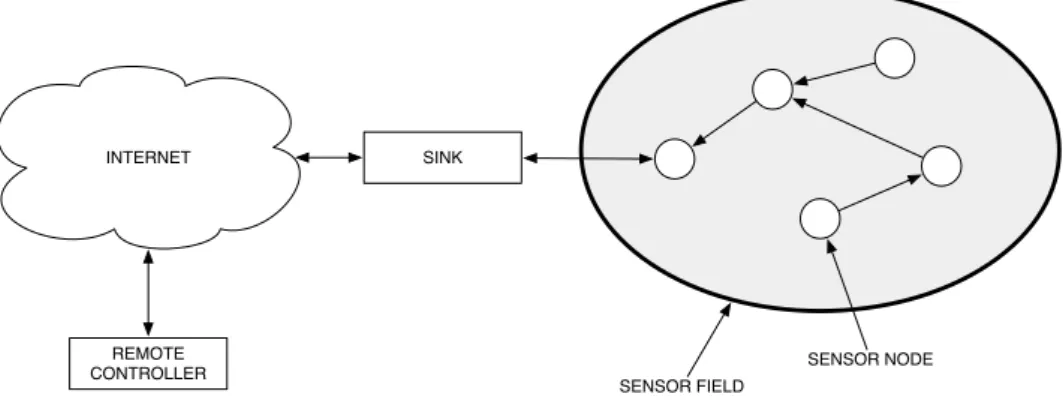
INTERNET SINK
SENSOR FIELD
SENSOR NODE REMOTE
CONTROLLER
Figure 2.1: Typical sensor network architecture
For all the scenarios seen in Section 2.1 we ideally aim to have nodes active and monitoring, unattended, for months or years. It is important to notice how the nodes are all interconnected each other and, especially for tree-based routing topologies, the correct delivery of data depends on all the nodes on the path toward the sink. Thus in many deployment it is not really important the average node lifetime but rather the minimum node lifetime, since the failure of a single node can determine the failure of the whole network.
In the analysis for energy consumption we will refer to a well-defined network model for a data collection network. The network consists of one sink and a large number of deployed sensor nodes. Data are transferred from the nodes to to the sink through a multi-hop transmission. As seen in Section 2.1.1 the network is intended to be static with a tree-based routing protocols whose routes
are calculated off-line. On the other side we can think to the typical sensor node as composed of four main components:
1. power supply subsystem to power the whole system
2. sensing subsystem including one or more sensor (with associated ADCs) for data acquisition and digitalization
3. processing subsystem composed by a micro-controller with memory for data storage
4. radio subsystem for wireless data communications
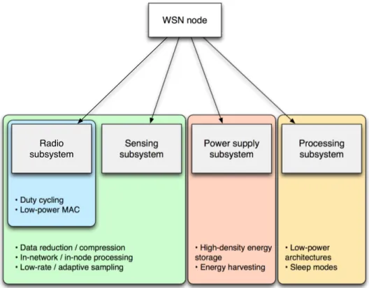
• Data reduction / compression • In-network / in-node processing • Low-rate / adaptive sampling
• High-density energy storage • Energy harvesting • Low-power architectures • Sleep modes WSN node Sensing subsystem Power supply subsystem • Duty cycling • Low-power MAC Processing subsystem Radio subsystem
Figure 2.2: Wireless sensor node power model. For each subsystem some of the major techniques for power consumption reduction are listed
Depending on the specific applications, the sensor nodes may also include additional components such as actuators or GPS. However, as these components
are optional, they are occasionally used and are not taken into consideration in this thesis.
Several approaches have to be exploited, even simultaneously, to reduce power consumption or increase lifetime in wireless sensor networks as better depicted in Figure 2.2. Some techniques are just related to one specific subsystem like energy harvesters for power supply or the low-power architectures for the processing subsystem. The sensing subsystem and the radio subsystem are strictly inter-related: the first one provides data to be sent using radio transmissions thus a reduction in the data size reflects in a reduction of power spent in transmission. Specific techniques, however, are specific for the radio subsystem such as duty cycling or the usage of low-power MAC protocols.
In the next paragraphs and chapters we are going to focus on each subsystem and on the major techniques related to that subsystem for energy consumption reduction.
2.3 Battery and power supply
Overall battery capacity is measured in milli-Amp-hours (mAh) or Amp-hours (Ah). In theory a rating of 3 Ah means the battery can supply 3 A for 1 hour or 1 A for 3 hours. In practice this in not always true. Due to battery chemistry, voltage and current levels vary depending on how the energy is extracted from a battery. Sometimes the battery is not quite empty, but there is insufficient potential energy in the battery to get the remaining charge out, for this reason a battery is said to be empty when the potential or voltage drops below a certain level. Typically, for a 1.5 V cell such as a AA-sized cell, the battery is considered empty when the voltage drops to around 0.9 V.
Even thought the technology is trying to scale down size and weight of the batteries used in sensor networks, with the actual technology batteries still are a significant fraction of the total size and weight of the nodes. Due to this strict relation between size and energy storage capacity we can characterize the batteries namely by energy density. The energy density is a term used for the amount of energy stored in a given system or region of space per unit of volume. On the other hand the power density is the amount of power per unit of volume.
Battery Type Wh/Kg J/Kg Wh/L Lead-acid 41 146000 100 Alkaline long-life 110 400000 320 Carbon-zinc 36 130000 92 NiMH 95 340000 300 NiCad 39 140000 140 Lithium-ion 128 460000 230
Table 2.1: Energy and power density for the most common battery technologies for WSNs
While an ideal energy reservoir should offer both a high energy and a high power density, the typical battery usually features high energy density but a limited power density.
The three main technologies traditionally used in WSNs are Alkaline Batteries, Lithium Batteries and Nickel Metal Hydride (NiMH) Batteries [McDowall,2000]. In Table 2.1 are reported the energy and power density for the most common battery technologies.
The Alkaline batteries are far the most common type of household battery, and they are very good for a variety of electronics applications. Alkaline batteries are low cost, widely available, and are ideal for low current applications at room temperature. However, they have two major shortcomings: the energy capacity is highly dependent on temperature and they don’t tend to work as well under high current draws.
For the Lithium batteries there are many varieties. Although it is difficult to put them all in the same class or use the same model to describe their behavior, there are some common characteristics. For the sake of this discussion, we will focus on the iron-disulfide formula in particular because it is the most common Lithium battery available in AA sizes. This type of battery is regularly used as a replacement for alkaline batteries where longer life, higher current draw, or improved temperature performance is needed. Even thought Lithium iron-disulfide batteries are not rechargeable, the big benefit to Lithium disposable batteries is that they do much better under low temperature and high current rate conditions.
maintain its characteristics through many recharges. Its biggest shortcomings are that it is relatively heavy and that it has a lower energy density, meaning that a typical AA-sized NiMH battery will start at 1.2 V instead of the conventional 1.5 V for an alkaline AA battery.
Recently new technologies have been proposed to try to further shrink down size and at the same time to increase the energy density of the batteries commonly used in very small size portable devices such as wearable and sensor nodes. These new batteries are based on new technologies like thin-film ion or Lithium-polymer cells [Owen, 1996]. They are similar to lithium-ion batteries, but they are consisting of thin materials, some only nanometers or micrometers thick, which allows the finished battery to achieve millimeters thickness. The problem with the thin-film batteries is that these batteries are too small for long lasting operations in sensor networks.
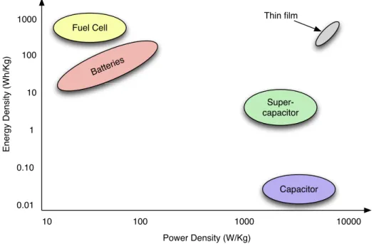
1000 0.01 10 10000 Energy Density (Wh/Kg) Power Density (W/Kg) Fuel Cell Batteries Capacitor Super-capacitor 100 1000 0.10 1 10 100 Thin film
Figure 2.3: Ragone plot power density / power energy plot for typical energy storage technologies
One of the most promising alternatives is the fuel cell [Chraim and Karaki,
Hydro-gen) to generate electrical power. FC has a very high energy density if compared to batteries, however the FC cannot respond to sudden changes in the load, thus a system powered solely by the FC is not enough. For this reason a hybrid system where the FC is used to recharge conventional batteries or a super-capacitor is a better solution. The gravimetric energy density of fuel cells is expected to be three to five times larger than Li-ion cells and more than ten times better than Ni-Cd or Ni-MH batteries whereas the volumetric energy density is six to seven times larger than Li-ion. Figure2.3shows the Ragone plot for the aforementioned storage systems that helps in understanding the relationship between batteries and capacitors.
In practice no single type of storage element can simultaneously fulfills all of the desired characteristics of an ideal storage system, thus a hybrid solution could overcome the limit of single reservoir and prove to be very much more efficient [Porcarelli et al., 2012].
Nowadays another solution begins to take hold in WSNs to extend the life-time of node and recharge the batteries: the usage of renewable energy to generate electricity [Morais et al., 2008][Thomas et al., 2006]. The big variety of energy sources in the environment potentially suitable for energy harvesting has driven increased interest in research community. The main sources used for harvesting include solar energy (as well as artificial lightning), vibrations (harvested using piezoelectric, electro-magnetic and capacitive converters), kinetic energy (avail-able in moving water in rivers, pipes and wind flow), magnetic fields (surrounding AC power lines), pressure and heat differentials (harvested using thermoelectric elements). However, due to practical constraints or challenges raised by the low energy density, target power requirements and, in some cases, feasibility of the energy harvesting method, many of these sources could not be considered for energy harvesting [Zhang et al., 2011].
How we can infer from Table 2.2 solar energy is the most efficient natural energy source available for sensor networks in outdoor applications [Brunelli et al.,
2009].
All the considerations on battery, harvesting and power supply brings to a power supply unit architecture as depicted in Figure2.4. This exemplified power unit is composed by the following blocks:
Platform Power Sources Converters Power Management Interface Output Buck-Boost Converter Batteries Supercaps Recharger MCU Fuel Cell
Figure 2.4: Complete power supply architecture for wireless sensor nodes
• Energy storage: the output and storage stage implements a double func-tion: it receives the energy from the conversions circuits and stores this energy in specific storage elements (batteries, super-capacitors, etc...). • Energy transduction: to adapt the system to different scenarios,
envi-ronments, energy sources and different sensor nodes.
• Fuel cell: this stage is used to recharge the storage elements when the energy can not be harvester and the storage elements are almost empty. • Power unit monitor: the interactions among the various stages are
Harvesting technology Power density Solar cells (outdoors at noon) 15 mW/cm2
Piezoelectric (shoe inserts) 330 µW/cm3
Vibration (small microwave oven) 116 µW/cm3
Thermoelectric (10 C gradient) 40 µW/cm3
Wind 10W/m2 at 2.5 m/s
Table 2.2: Power density for different energy harvesting sources
such as measuring the charge status of the storage elements, measuring the voltage levels given by the transducers and the conversion electronics. • Interfaces: the goal of the interface is to provide adequate information for
power management and power policies implementation.
2.4 Radio and communication network
In general, wireless networks can be divided in two main categories: infrastruc-tured and ad-hoc networks. Wireless sensor networks are a special case of ad-hoc networks.
Infrastructured networks The principal characteristic of this type of net-works is that they always have one or more central coordination points. The most famous example for this type of networks is the cellular network where each node, to communicate each other, needs to negotiate with the infrastructure hardware of the cell it belongs to [Rahnema, 1993]. Once this communication has taken place the infrastructure takes care of setting up a channel between the peers. In cellular networks the communication between two peers must pass throughout the network infrastructure also if the two devices could be able to communicate to each other because they are in the transmission range of each other.
Ad-hoc networks Differently from infrastructured networks, ad-hoc networks are totally self-organizing and do not relay on a stable infrastructure to enable the communication. Any activity promoted by peers inside the network is carried on
(a) WSN without sink (b) WSN with one sink
Figure 2.5: Different WSN architectures. (a) There is no sink and the nodes communicate directly with the destination node after query. (b) Sink collects data from the sensors via multi-hop communication and forwards collected data to a remote destination
without a central point for coordination. All the peers of an ad-hoc network can play two different roles: (1) the end-point of an active communication (sender or receiver) and (2) the intermediate routing point along the path of an active com-munication, performing the routing of data for the other peers’ communications. In this type of network we can identify three types of communication pattern: broadcast, convergecast and local gossiping. Broadcast is generally used by a base station (sink) to transmit some information to all the sensor nodes of the net-work (broadcasted information may include queries of sensor, program updates, etc...). In some scenarios, as introduced in Section 2.1.2, the sensors that detect an intruder communicate with each other locally. This type of communication pattern is called local gossiping where a sensor sends a message to its neighboring nodes within a range. Lastly convergecast is the communication pattern where a group of sensors communicate to a specific sensor or sink.
2.4.1 WSN architecture
Besides the two kind of networks seen in Section2.4, the WSNs can be considered as a special kind of ad-hoc networks [Akyildiz et al.,2002]. In fact in WSNs each sensor has too little available power to be useful if used alone. Actual WSNs are made up of hundreds (or maybe thousands) of sensors. All sensors cooperate to provide sensing, communication and reliability to all the system.
In WSNs for data collection each node is able to acquire data from the envi-ronment, eventually perform some kind of transformation on the acquired data and send out data toward the external world. This can happen in two ways: either every node can communicate to the user or only few nodes can do that. In Figure 2.5 a graphical explanation oh the two cases.
In the first case we can think that each node has enough power to directly communicate the result to the destination point (i.e. using a satellite up-link or GSM connection) or each node can wait to be directly in communication with the destination peer before sending out the data (i.e. a mobile device can directly query the nodes in the network). This case where the communication takes place directly between the sender and the receiver is called single-hop communication and it is fairly rare in WSNs.
Nevertheless the most common is the second case: in the network there are one or more special nodes, namely the sink nodes, which aim is to collect and communicate data to the end user. Usually these nodes are structurally different from the nodes of the network having more computational power and battery. They act like gateways between the user and the WSN and they have usually two interfaces: one toward the WSN for data gathering and the second one used by user to interrogate the network and to extract the needed information. Since the data has to be delivered to the sink that could be physically away for the sensing node, data is routed through all the intermediate nodes on the path toward the sink, in a multi-hop communication.
2.4.2 Energy consumption in radio subsystem
The radio subsystem is the most important system in a wireless sensor node since it is the primary energy consumer in all the application scenarios [Raghunathan
et al., 2002]. In general the communication subsystem has a much higher energy consumption than the computation and sensing subsystems. Transmitting one single bit of data consumes as much energy as executing thousands instructions [Shih et al.,2001]. Moreover the radio energy consumption is of the same order in the reception, transmission, and idle states, while the power consumption reduces a lot when the node (and the transceiver) is put in sleep mode. It is clear that the radio has to be managed wisely in order to extend the lifetime of the sensor node and the whole network.
Not all the energy spent by the communication subsystem is wasted and it is possible to identify at least five different cases in which the energy is wasted by radio communications [Demirkol et al., 2006]:
• Idle listening. A node is said to be in idle listening when it listens on an idle channel in order to receive possible traffic.
• Collisions. A collision occurs whenever a node receives more than one packet at the same time. Each time there is a collision, the packet has to be discarded and the packet retransmitted, increasing the energy consumption. In general it is possible to identify two types of collisions: (1) direct collisions and (2) indirect collisions.
Direct collisions occur when two or more nodes sending data are in the transmission range of each other and send their data at approximately the same time towards a common receiver as in Figure 2.6a.
Indirect collisionsoccur when two or more nodes cannot hear each other but have overlapped transmission ranges and send data at approximately the same time as depicted in Figure2.6b. In this case there is the so called hidden terminal problem where the nodes in both the transmission ranges of the two sending nodes receive only junk transmission.
• Overhearing. A node receives packets that are destined to other nodes. This problem usually arises when a large number of devices try to commu-nicate in the same area. In this case the communications collide frequently and a channel contention problem may rise when many nodes share the same sub-area and all the nodes are able to communicate each-other.
R B G
(a) Direct collision
R G B
(b) Indirect collision (hidden terminal problem) Figure 2.6: Different collisions in WSNs. (a) Two nodes are in the transmission range and send data at the same time colliding at node G. (b) Two nodes are not in transmission range but they send data approximately at the same time and again there is collision at node G
• Control-packet overhead. This is due to protocol implementations since a minimum number of control packets are required to make the communi-cation feasible.
• Over-emitting. It is caused by the transmission of a message when the destination node is not ready. This problem arises when the network syn-chronization is lost and the nodes are not able to exchange packets.
2.4.3 Energy saving in wireless communications
Duty cycling is the major technique for energy saving in wireless communications [Sadler, 2005]. Normally, a sensor radio has 4 operating modes: transmission, reception, idle listening and sleep. Measurements showed that the most power consumption is due to transmission and in most cases, the power consumption in the idle mode is approximately similar to receiving mode. On the contrary, the energy consumption in sleep mode is much lower. That is the most energy-conserving operation is putting the transceiver in this state whenever the com-munication is not required. Ideally we could turn on the radio as soon as a new data packet becomes available for sending and switch off it again when the data
is sent. This behavior is namely referred to as duty cycling and the duty cycle is defined as the time that the radio spends in an active state as a fraction of the total time under consideration.
The problem with this technique is that in collaborative networks such as WSNs, a coordination among nodes is required to enable data exchanging and forwarding. Thus a sleep / wakeup scheduling algorithm is required to permit the correct functioning of the network. The scheduling can be implemented in two different fashions: (1) on top of an existing MAC protocol (at network or application layer) or (2) strictly integrated within the MAC protocol itself.
In the next section we want to investigate this second case. 2.4.3.1 Low-power MAC protocols for WSNs
The MAC protocol is extremely important in WSN since it creates the network infrastructure by defining the communication channels and shares available com-munication among nodes. As seen before the radio comcom-munications are the most energy expensive actions so the MAC protocol should be properly designed to offer energy saving opportunities by cutting down energy inefficient access to medium.
Besides the energy efficiency other important attributes for MAC protocols are scalability and adaptability to changes. This is because changes in network size or topology are common in WSNs, especially considered the limited node lifetime of the wireless nodes. Moreover the addition of new nodes to the network should be handled rapidly and effectively for a successful adaptation [Wan et al., 2008]. A good MAC protocol should gracefully accommodate such network changes. Other typical important attributes such as latency, throughput and bandwidth utilization may be secondary in sensor networks. Contrary to other wireless networks, fairness among sensor nodes is not usually a design goal, since all sensor nodes share a common task.
The MAC protocols designed to integrate scheduling policies and power man-agement techniques can be categorized in three different categories: (1) contention-based, (2) TDMA-based and (3) hybrid.
Access (CSMA) or better on Carrier Sense Multiple Access / Collision Avoidance (CSMA/CA). Nodes using contention-based MAC do not require coordination among nodes in accessing the communication channel. When a node needs to send data, it verifies the absence of other traffic before transmitting. If the channel is sensed busy before transmission then the transmission is deferred for a random interval. This reduces the probability of collisions on the channel. Colliding nodes will back off for a random duration of time before attempting to access the channel again.
In TDMA-based (Time Division Multiple Access) protocols there is an ex-plicit synchronization among the nodes in the network. The scheduling offers a collision-free scheme by assigning each node a well defined time slot in which communication is permitted. This synchronization avoids interferences between adjacent nodes and, consequently, the energy waste coming from packet collision [Arisha,2002]. Moreover TDMA-based MAC protocol are immune to the hidden terminal problem seen in Section 2.4.2 since the time slot of each node is unique among its neighbors.
Hybrid MAC protocols have the advantages of both contention-based MAC and TDMA-based MAC protocols. While control packet are transmitted in the random access channel, data packets are transmitted in the scheduled access channel, in this way hybrid protocols can obtain higher energy saving and offer better scalability and flexibility.
In the following paragraphs are few of the most common low-power MAC protocols opportunely designed for wireless sensor networks.
Sensor-MAC (S-MAC) To solve the energy wasting problem the S-MAC [Song et al., 2008] alternates two different states: active state and sleep state, that is periodically listening and sleeping. S-MAC actually reduces the listening time by letting the node go to sleep into periodic sleep mode. Nodes exchange sync packets to coordinate their sleep / wakeup periods and neighboring nodes form virtual clusters to set up a common sleep schedule. If two neighboring nodes reside in two different virtual clusters, they wake up at listen periods of both clusters. The channel access time is split in two parts. In the listen period nodes exchange sync packets and special control packets for collision avoidance
while in the remaining period the actual data transfer takes place. Considering that the sender and the destination have to be awake and talk to each other, this brings in a problem since periodic sleep may result in high latency especially for multi-hop routing algorithms, since all immediate nodes have their own sleep schedules. The latency caused by periodic sleeping is called sleep delay. To avoid high latencies in multi-hop environments S-MAC uses an adaptive listening scheme. A node overhearing its neighbor transmissions wakes up at the end of the transmission for a short period of time. If the node is the next hop of the transmitter, the neighbor can send the packet to it without waiting for the next schedule. TA TA TA NORMAL S-MAC T-MAC Active Sleep
Figure 2.7: Comparison between S-MAC and T-MAC
Timeout-MAC (T-MAC) The problem of sleep delay resulting in high laten-cies as seen for S-MAC is partially solved in the so called Timeout-MAC (TMAC) [Farjaudon and Hascoet,1988] that results particularly useful under variable traf-fic load. In T-MAC listen periods end when no activation event has occurred for a time threshold TA. A comparison between S-MAC and T-MAC is in Figure 2.7. D-MAC Although duty-cycle based MAC protocols are energy efficient, they suffer sleep latency, i.e., a node must wait until the receiver wakes up before it
RX TX RX TX RX TX RX TX RX TX RX TX RX TX RX TX sleep sleep sleep sleep
Figure 2.8: A data gathering tree using D-MAC protocol
can forward a packet. This latency increases with the number of hops. In ad-dition, the data forwarding process from the nodes to the sink can experience an interruption problem. This is why the data forwarding process in S-MAC and T-MAC is limited to a few hops. When dealing with deep static tree-like networks, these MAC protocols show their limitations. In this type of networks convergecast is the mostly observed communication pattern within sensor net-works. These unidirectional paths from possible sources to the sink could be represented as data gathering trees. D-MAC [Kebkal et al., 2010] is an adaptive duty cycle protocol that is optimized for data-gathering in tree-like networks. In D-MAC based networks the nodes schedules are staggered according their posi-tion in the data gathering tree. Each node has a slot which is long enough to permit data transmission hence, during the receive period of a node, all of its child nodes has transmit periods and contend for the medium. Low latency is achieved by assigning subsequent slots to the nodes that are successive in the data transmission path as in Figure 2.8.
Traffic-Adaptive MAC Protocol (TRAMA) One of the most important energy-efficient TDMA protocol for wireless sensor networks is TRAMA [I and Pollini,1994]. TRAMA divides time in two portions, a random-access period and a scheduled access period. The random access period is devoted to slot reservation
and is accessed with a contention-based protocol. On the contrary, the scheduled access period is formed by a number of slots assigned to an individual node. The slot reservation algorithm is composed by a series of subsequent steps. First the nodes derive the two-hop neighborhood information. This information is used to create a collision free scheduler. Afterwards the nodes start an election procedure to associate each slot with a single node. A node becomes the owner of the slot only if its priority, calculated as a hash function of the node identifier and the slot number, is the highest priority among all the nodes. Finally nodes send out a synch packet containing a list of intended neighbor destinations for subsequent transmissions. Consequently nodes can agree on the slots which they must be awake in.
Other low-power MAC protocols Among the TDMA-based MAC proto-cols it is possible to find: FLAMA (FLow-Aware Medium Access) [Rajendran et al., 2005], LMAC (Lightweight MAC) [Lee et al., 2008], AI-LMAC (Adaptive Information-centric LMAC) [Chatterjea et al., 2004], SPARE-MAC (Slot Peri-odic Assignment for Reception MAC) [Turati et al.,2009], DEE-MAC (Dynamic Energy Efficient MAC) [Cho et al., 2005]. For contention-based MAC protocols we have: B-MAC (Berkeley MAC) [Fakih et al.,2006], U-MAC (Utilization-based MAC) [Yang et al., 2005]. Hybrid MAC protocols: Z-MAC [Rhee et al., 2008], Wise-MAC [El-Hoiydi and Decotignie, 2004], PTDMA (Probabilistic TDMA) [Oikonomou and Stavrakakis, 2004].
2.4.3.2 Duty cycling on top of MAC protocols
As seen in Section2.4.3sleep / wakeup schemes can be defined also as independent protocols (network or application layer) on top of existing MAC protocols. This protocols are usually divided into three main categories: on-demand, scheduled rendezvous and asynchronous schemes.
The basic idea of on-demand protocols it that a node should wakeup only when another node wants to communicate with it. The real problem with this approach is how to inform the sleeping node that a child node is willing to communicate. Sometimes the best solution is to implement a wake-on-radio mechanism where a second low-rate and low-power radio or analog circuit is used for signaling and
wakeup while a more powerful and more energy hungry radio is used for data transmission.
An alternative solution consist in using a scheduled rendezvous approach. The idea is that each node should wake-up at the same time as its neighbors. The wakeup time is scheduled and the node remain active just for the short time interval needed to communicate with their neighbors before going back to sleep and waiting until the next rendezvous time.
Finally an asynchronous sleep / wakeup protocol can be used. In this case a generic node can wake up when it wants and it is still able to communicate with its neighbors. This is possible by guaranteeing that neighbors always have overlapped active periods within a specified number of cycles.
These technique for power management are usually implemented on top of an existing MAC protocol. For low-power WSNs the most common protocol is the IEEE 802.15.4.
IEEE 802.15.4 The IEEE 802.15.4 protocol is a standard for rate low-power Personal Area Network (PAN). A PAN is composed by a coordinator which manages the whole network (sometimes it is possible to have several coordinators managing subsets of the nodes in the network). Each node in the network must associate with the PAN coordinator in order to communicate. In the original standard the only supported network topologies are: star (single-hop), cluster-tree and mesh.
The IEEE 802.15.4 protocol [Zheng and Lee, 2003] supports two operational modes that may be selected by the PAN coordinator: (1) the non beacon-enabled mode in which the MAC is simply ruled by non-slotted CSMA/CS and (2) the beacon-enabled mode in which beacons are periodically sent by the coordinator to synchronize nodes that are associated with it. These beacons provide an energy management mechanism based on a duty cycle.
In beacon-enabled mode the coordinator defines a superframe structure as in Figure 2.9 which is constructed defining: (1) the Beacon Interval (BI) which defines the time between two consecutive beacon frames, (2) the Superframe Du-ration (SD) which defines the active portion in the BI, and is divided into 16 equally-sized time slots during which frame transmissions are allowed.
0 1 2 3 4 5 6 7 8 9 10 11 12131415
CAP CFP Inactive Period
beacon beacon
GTS1 GTS2
SD (active)
Beacon Interval (BI)
Figure 2.9: Superframe structure for IEEE 802.15.4 protocol
Optionally, an inactive period is defined if BI > SD. During the inactive period all nodes may enter in sleep mode.
BI and SD are determined by two parameters, the Beacon Order (BO) and the Superframe Order (SO), respectively, as
BI = aBaseSuperf rameDuration· 2BO
SD = aBaseSuperf rameDuration· 2SO
)
for 0 SO BO 14 (2.1) aBaseSuperf rameDuration = 15.36 ms denotes the minimum duration of the superframe, corresponding SO = 0.
During the SD, nodes compete for medium access using slotted CSMA/CA in the Contention Access Period (CAP). For time-sensitive applications, IEEE 802.15.4 enables the definition of Contention-free period within the SD, by allo-cation of Guaranteed Time Slots (GTS). It can be easily observed that low duty-cycles can be configured by setting small values of the superframe order (SO) as compared to beacon order (BO), resulting in greater sleep (inactive) periods.
The advantage of this synchronization with periodic beacon frame transmissions from the PAN coordinator is that all nodes wake up and enter in sleep mode at the same time. However using this synchronization scheme in a cluster-tree net-work with multiple coordinators sending beacon frames, each with its own beacon interval, is a challenging problem due to beacon frame collisions.
2.4.3.3 Case study: Conservative Power Scheduling
The most common scheduled rendezvous scheme for tree-based networks is the staggered wakeup pattern [Keshavarzian et al., 2006] where nodes located at dif-ferent levels of the data-gathering tree, wake up at different times. This approach is much more flexible than the classical fully synchronized pattern in which all the nodes of the network wake up at the same time according to a periodic pattern as seen in Section 2.4.3.1for S-MAC and T-MAC. On the contrary the staggered wakeup pattern takes advantage of the internal organization of the network by sizing the active times of different nodes according to their position in the data gathering tree.
The staggered scheme has the advantage that at different times, only a subset of the nodes are active thus the probability of collisions is potentially lower than for the fully synchronized pattern, since only few nodes contend for the channel access at the same time. As seen in Section 2.4.2 this permits a reduction in the power consumption since the active period of each node can be significantly shorter. This scheme enables also mechanisms of data aggregation since the parent nodes can wait to receive data from all their children before forwarding to the next node in the path.
The major problem with the staggered scheme is that nodes located at the same level in the gathering tree wake up at the same time so collisions still are a problem. Moreover the scheme has limited flexibility due to the fixed duration of the active and sleep periods that are usually the same for all nodes in the network.
Ideally a low-power protocol should be able to allow different active and sleep times for different nodes in the gathering tree according to the different amount of data managed by the single node.
Following this principle in this paragraph a new power management protocol derived for the staggered wakeup pattern is presented. This protocol, namely Conservative Power Scheduling (CPS) protocol, is built on top of IEEE 802.15.4 MAC protocol and tries to adapt a slotted approach derived from TDMA schemes to the staggered pattern already presented.
In the following description we will refer to a data collection paradigm where data typically flows from source nodes to a sink node. Nodes are organized in the network to form a static tree rooted at the sink. The routes in the tree are static and each parent node has to be physical neighbor of all its children. Even though it is possible to assume that the routes are static for a long period, the paths can re-computed periodically to take into account variation in the network topology.
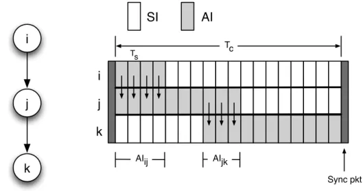
Time is assumed to be divided in time slots of duration Ts. Slots are arranged
to form period cycles, namely the communication periods, where each cycle is made up of m slots and has a duration of Tc = mTs. Each communication period
is divided into two parts: an Active Interval (AI) during which the node must keep its radio on to receive / transmit from / to other nodes, and the Sleep Interval (SI) during which nodes are sleeping, both periods are multiple of the time slot Ts. To permit data exchange, the talk interval between a node and its
parent / child must overlap in at least a time slot Ts as clarified in Figure2.10.
Consider for example a generic node j having node i as parent and node k as child. If Tc is the communication period, AIij the overlapping active interval
between nodes i and j, AIjk the overlapping active interval between j and k, then
to ensure the protocol correctness we have to assure that:
AIij + AIjk Tc (2.2)
The cycle of duration Tc is the same for all the nodes in the network thus
a synchronization is required for the entire network. The most simple method to guarantee synchronization among all the nodes in a tree-based network is to use a synchronization packet sent in broadcast by the tree coordinator. Each synchronization broadcast packet delimits the cycle period Tc
i j k i j k Tc Ts AIij AIjk AI SI Sync pkt
Figure 2.10: Conservative Power Scheduling parameters and communication model
When the CPS protocol is used, to reduce the probability of collisions in the network each time slot Ts is uniquely assigned to a specific node in the whole
net-work. This restriction practically reduces to zero the probability of collision but, on the other hand, it increases the latency experienced by packets to reach the root node. In data-gathering networks for data collection this is not a real issue since the inter-sampling period (in the order on tenth of minutes) is usually ex-tremely larger than the gathering time, thus in this scenario it is more important to preserve the integrity of data avoiding collisions than low data latency.
The real challenge in CPS protocol is to correctly assign the time slots to each node such as to minimize the power consumption. To achieve this goal each node has to be in the active interval for the shortest time possible, waking up just in time for sending sampled data to the parent node and going back to sleep as soon as it has forwarded all the data coming from its child nodes. Differently from other approaches found in literature [Hohlt et al., 2004][Lu et al., 2004], CPS does not calculate adaptively or run-time the slots scheduling but it uses a static scheduler computed off-line. The algorithm for slots assignment takes in input the tree-structure (parent-children relationships for all the nodes) of the network