1
Financial fragility and income inequality
Ph.D. candidate: Francesco Ruggeri
Supervisors: Claudio Sardoni, Marco Veronese Passarella
XXXII Ph.D. cycle
Economics and Finance Ph.D. program
Department of economics and social science
3
Introduction
After the financial crisis of 2007/2008 academics and policymakers have turned their attention to how private debt can affect, significantly, the economic performance of a country.
In the period of the “Great Moderation”, the increasing level of income inequality, together with structural transformations, has created an environment where a large portion of the private sector was more prone to rely on bank credit in order to finance its expenditure. While borrowing can have a first expansionary impact, because of the increase in the purchasing power of the borrowers, the increase in the stock of debt in the “medium-term” can have different negative effects. Debt repayment transfers resources to “high propensity to spend” agents (borrowers) to “low propensity to spend” agents (lenders). The impact of this income transfer can have a negative impact on final expenditure and, thus, on GDP. The increase in the stock of debt leads to an increase of the fragility of the household sector because of its increase in the vulnerability to different kind of shocks such as: an increase of the interest rates, a sudden decrease of the disposable income, a collapse of the assets used as collateral, and to possible changes of the attitudes of the lenders.
Starting from this, we developed three different theoretical models in order to describe the impact of an expansion of household debt, in an environment of high-income inequality.
The thesis is divided into three chapters. In the initial part of every chapter there is a description of different aspects of the increase in household debt during the period preceding the financial crisis of 2007-2008.
In the first chapter, the problem of household debt is addressed looking at the possible causes of the increasing willingness of households to finance their spending by borrowing and at the expansionary and contractionary effect of debt. The second part of the chapter contains a model that shows the Janus-like faces of household debt.
The model is composed of three sectors: a firm sector, a banking sector, and the households sector. The households sector is divided into two subsectors in order to detect differences in income and wealth and propensity to consume.
One of the main interesting results of the model is that: borrowing to finance consumption increases the level of aggregate demand and income like in a standard Keynesian model and in the multiplier-accelerator model by Samuelson, but at the same time fresh borrowing increases the level of the stock of debt, which has a negative impact on demand has it implies a transfer of resources from the high propensity to consume borrowers to lower propensity to consume lenders. The model is able to replicate a debt-driven cycle created by the interaction of the flow and the stocks effect of household debt.
The second chapter starts with a description of some crucial evolutions in place during the Great Moderation in the U.S. economy: the evolution of the financial sector, the increase in income inequality, changes in the attitudes towards consumption and in the use of debt of the households sector, and the long term trend of households’ expenditure in US.
The second part of the chapter, contains a model which is an extension of the one in the first chapter. The model has three sectors: a household sector, goods market firms and firms who produces houses, and a banking sector. The focus is on the between the household sector, the
4 housing market, and the banking sector. Households are split into two sub-sectors in order to describe the implications of differences in income and wealth. An emulative consumption function and demand for houses is introduced in order to detect the impact of income inequality on spending and demand for loans. With two different shocks on credit access, we are able to replicate the boom and bust dynamics of debt led expansions and a financial accelerator dynamics where the interaction between the housing market, the banking sector, and the households sector generates a feedback loop that creates a cycle.
In the third chapter, the problem of household debt is studied looking at the international level. In the first part of the chapter, there is a description of the different demand regimes that have emerged during the period of the so-called financialization. In the second part, a two-economy model is presented. Each of the two economies has four sectors: households, banks, firms, and a government with its central bank. Like in the first two models, the household sector is divided into two subsectors to study the implications differences in income, consumption and investment behavior.
We perform two different experiments, in the first one we let the supply of credit in one country increase in order to detect what is the “international” impact of a credit supply shock. In a second experiment, we study the different effects of an income distribution shift when households have different access to credit.
The modelling methodology used is based on the Stock-Flow Consistent approach. This new class of models is very suitable to study the effect of financial variables on the economy because they focus their attention explicitly on the “sustainability” of the pattern of financial flows and the subsequent accumulation of stocks.
5
Household debt, aggregate demand, and instability in a stock-flow
consistent model
1. Introduction
Since the start of the Great Moderation period, Anglo-Saxon countries and other advanced economies have experienced a dramatic increase of household debt, both in absolute terms and in terms of debt-to-income ratios. The increase in the stock of debt for the households was due to the need for middle and low-income households to borrow in order to “keep up with the Jones” and run to stand still in the face of stagnation or a reduction of their income. Debt-led consumption was very important because allowed these economies, especially the US and UK, to solve, at least temporarily, the aggregate demand problems generated by the shift of income distribution in favour of the high-income part of the population.
After the Housing Bubble’s burst in the US consumption collapsed and households started to deleverage putting contractionary pressures on the economy. The collapse of consumption can be seen as one of the main drivers of the stagnation and the slow growth in the aftermath of the financial crisis.
Starting from these stylized facts, the Stock-Flow Consistent model that we developed tries to describe the effect of an increase of household debt on the steady-state solution of the model and the ability of debt to generate fluctuations affecting the dynamics of aggregate demand. The model comprises three sectors: a firm sector, a banking sector, and the household sector. The household sector is split into two in order to detect differences in income and wealth and propensity to consume. Particular attention is given to the consumption and demand for loans as the model tries to describe the evolution of consumption and borrowing practices that occurred in the last thirty years.
Money is endogenous in the model as banks respond to the demand for credit expanding their balance sheets. The presence of endogenous money makes the model more unstable as the impact of fresh borrowing on overall spending is larger compared to standard loanable funds models. The model is able to show the Janus-like faces of household debt: borrowing to finance consumption increase the level of aggregate demand and income, as in the standard Keynesian model and in the multiplier-accelerator model by Samuelson, but at the same time fresh borrowing increase the level of the stock of debt. The stock of debt puts contractionary pressure on the aggregate demand because the repayment affects money balances and transfers resources from high propensity to spend agents, to low propensity to spend agents.
The interaction of these phenomena creates a “predator-prey” type model in which fresh borrowing increases income, which feeds the ability to borrow more and consume; at the same time, the stock of accumulated debt “preys” on income due to the contractionary forces of the repayment mechanism.
The structure of the paper is the following: in section two we use descriptive statistics to describe the evolution of households’ debt in some advanced economies. Data shows how households’ debt has grown before the financial crisis and that after the crisis the level of debt has remained around high levels.
6 In section three, we present some different explanations of why households’ debt has grown. In section four, we describe the Janus-like effect of debt on the economic outcomes.
In section five and six we present a stock-flow consistent model that tries to replicate some of the dynamics we describe in section two and section three.
section seven concludes.
2. Descriptive statistics of the evolution of the household debt
Since the beginning of the so-called Great Moderation period, the period that started in the early ‘80s and ended with the start of the Global Financial crisis, some of the most advanced economies have seen the evolution of some common trends. The most important was the dramatic increase in the household debt. If we look at the evolution of the debt held on the balance sheet of the household sector in some Anglo-Saxon countries, we can see how it was steadily increasing during the period of the Great Moderation.
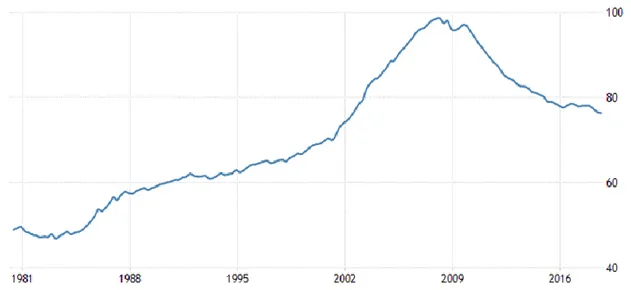
Fig. 1 shows the evolution of the household’s debt-to-GDP ratio in the USA. We can split the evolution of household debt into two phases: the first that goes from the early ‘80s to the late ‘90s and the second from the late ‘90s until the financial crisis. In the first phase households’ debt was growing slowly, in the second phase it ballooned, growing faster than the previous period.
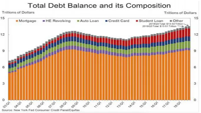
After the financial crisis, households’ debt started to decline following the deleveraging process, but, as shown in fig.2 in 2019 it was $869 billion higher than 2008’s trillion peak (Federal Reserve Bank of New York’s Centre for Microeconomic Data). This does not mean that the United States are in the same situation as before the financial crises. The debt-to-disposable income ratio has declined in the last years.
It is interesting to show how high level of debt are structural features of the US economy and this means that a decline in the disposable income can have important effect on the economy.
Fig. 1 Household debt-to-GDP ratio for the USA
7 Fig.2
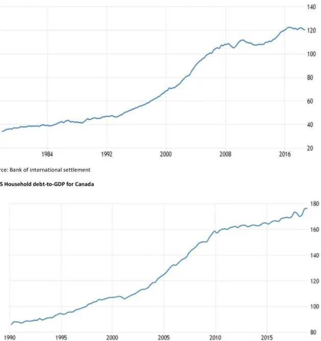
The evolution of the debt for the Household sector was the same for the United Kingdom, as shown by fig. 3 with a two-step process the first started in the early ‘80s and ended at the beginning of the ‘90s and the second one from the late ‘90s until the start of the financial crisis.
Fig. 3 Household debt-to-GDP for the UK
Source: Bank of international settlement
As for the USA, household debt-t-GDP started to decline after the financial crisis, but after few years, it rised again.
8
Fig. 4 Household debt-to-GDP for Australia
Source: Bank of international settlement
Fig. 5 Household debt-to-GDP for Canada
Source: Bank of international settlement
The difference is that household debt never really declines for both Australia and Canada. It started to increase from the early 90s in both countries and in Australia, after a brief decline during the financial crisis it rose again after few years. In Canada, the trend continued to be positive even during the financial crisis.
If we look at the debt-to-disposable income ratio for these four countries, we can see the same pattern.
9
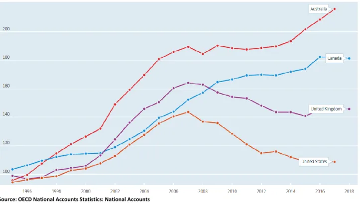
fig. 6 Household debtTotal, % of net disposable income, 1995 – 2018
Source: OECD National Accounts Statistics: National Accounts
Debt ratios rose rapidly in all the countries, the divergence began when UK and US started to deleverage after the financial crisis while Australia and Canada, albeit at a slower pace, continued with the debt accumulation
3. Different explanations of the increase in borrowing
Over the time several different theories have been suggested to explain this dramatic increase in the households’ borrowing; although none of them seem sufficient to describe exhaustively this phenomenon, they can be used together to understand the evolution of the dynamics we are studying.
The “mainstream” view of households’ borrowing and expenditure is based on the Life-Cycle Hypothesis1. Alternative explanations are based on Duesenberry’s relative-income hypothesis2, in
his work, he hypothesize that household consumption decisions are significantly affected by the income and consumption pattern of the rest of the economy, especially of the high income part of the households’ sector.
1 “Debt is accumulated by far-sighted, utility maximizing households whose objective is to smooth
consumption over a potentially infinite time horizon. From this perspective,
consumption spending should not be the cause of deep recessions because it implodes owing to
unsustainable patterns of household debt accumulation. Indeed, the life cycle hypothesis suggest that, in the limit, consumption follows a random walk Yun K. Kim & Mark Setterfield & Yuan Mei, 2014. "A theory of aggregate consumption," European Journal of Economics and Economic Policies: Intervention, Edward Elgar Publishing, vol. 11(1), pages 31-49, April
2 Duesenberry, J.S. (1949) Income, Saving and the Theory of Consumer Behavior, Harvard University Press,
10 Several empirical studies support the relative-income hypothesis: Luttmer (2005) and Alpizar et al (2005) show how individual well-being is crucially correlated with relative consumption as well as the absolute level of consumption. Even economist that usually used the permanent-income-hypothesis have started to incorporate the notion of relative income in their models. Dybvig (1995) shows how utility maximizing
households experience addiction effects, the result is that consumption rises in
response to increases in income are greater than falls in consumption related to reduction of income. Cuadrado and Van Long (2011) shows ho individual utility can be dependent on the utility of a specific reference group, so individual consumption is affected by the reference group’s income and consumption.3
Some authors have suggested that the increase in household debt was not only due to the increase in inequality, but also -at least in the case of the United States- to the increase in the trade deficit and to a conservative fiscal stance of the government. Households’ debt, and more in general private debt, was the only source of funding in an environment of a basically restrictive fiscal policy and a chronical deficit with the rest of the world. Wynne Godley described the evolution of the US economy in this way:
“During the last seven years a persistently restrictive fiscal policy has coincided with sluggish net export demand, so rapid growth could come about only as a result of a spectacular rise in private expenditure relative to income. This rise has driven the private sector into financial deficit on an unprecedented scale. The Congressional Budget Office (CBO) is projecting a rise in the budget surplus through the next 10 years, conditional on growth’s continuing at a rate fast enough to keep unemployment roughly constant, and this implies that it is government policy to tighten its restrictive fiscal stance even further (Congressional Budget Office 1999a, 1999c). At the same time, the prospects for net export demand remain unfavourable. But these negative forces cannot forever be more than offset by increasingly extravagant private spending, creating an ever-rising excess of expenditure over income[…]If, as seems likely, private expenditure at some stage reverts to its normal relationship with income, there will be, given present fiscal plans, a severe and unusually protracted recession with a large rise in unemployment. It should be added that, because its momentum has become so dependent on rising private borrowing, the real economy of the United States is at the mercy of the stock market to an unusual extent. A crash would probably have a much larger effect on output and employment now than in the past.”(Godley 1999, p. 216-217)
Nikiforos 2016 also described how households’ saving, and borrowing, must adjust in order to maintain high level of employment in an environment of fiscal consolidation, trade deficits and income inequality. As Nikiforos explained:
“An increase in income inequality and the current account deficit and a consolidation of the government budget lead to a decrease in the saving rate of the household sector. Such a process is unsustainable because it leads to an increase in the debt-to-income ratio of the households and its maintenance depends on some kind of asset bubble.”(Nikiforos 2016, p. 563-564)
11 While would be more accurate to take into account the external and the government sector in the rest of the chapter we limit our analysis to considering the relation between income inequality, changing households’ attitudes and households’ debt in a closed economy with no public sector. A more general analysis will be presented in chapter three.
In the next two sections we will present some literature based on the Duesenberry approach in order to explain the rise in the stock of debt in the balance sheets of the households’ sector during the great moderation period.
3.1 Changing institutions and attitudes
One possible explanation for the rise in the household debt can be based by looking at the evolution of factors like financial institution, financial and consumption practices and households' attitude. As pointed out by Cynamon and Fazzari, until the early 1980 the use of credit by households was limited to mortgages to finance “housing investment” or to credit line to finance “consumption” of cars4.
Since the late ‘70s, the attitudes towards borrowing started to change rapidly:
“The share of total consumer debt made up by revolving debt, which consists primarily of credit card balances, increased steadily up until 1998 when it reached about 46 percent. The number of consumers who have access to revolving credit has increased as well (Torralba 2006). Between 1970 and 1998, the proportion of all U.S. households that had at least one bank-type credit card grew from 16 percent to 68 percent.” (Cynamon and Fazzari 2008, p. 15)
Cynamon and Fazzari argue that during the Great Moderation period attitudes towards borrowing started to change:
“...Borrowing for a home with 20 percent down and a fixed-rate mortgage was consistent with the financial norms of the 1960s and the 1970s. However, few people in that era would re-finance their mortgages to get cash for a new car or a vacation. When home equity loans with tax advantages became available in the late 1980s, borrowing against one’s home for non-housing consumption became more common. In the 1990s, innovations in the mortgage markets reduced transaction costs and cash-out refinancing became more common. Initially, these actions were responses to changes in available financial products.We argue, however, that what households consider “responsible” behavior also evolved along with these changing practices.”(Cynamon and Fazzari 2008, p. 14) This increase in the willingness of borrowing by households was facilitated by the evolution of the banking and financial sector. The spread of new financial practices like the emergence of the “cash-out” refinancing option encouraged households to convert their “home equity” into cash, ready to be spent, rather than reducing the monthly debt service payments5.
4 Cynamon, Barry Z. and Steven M. Fazzari (2008). “Household debt in the consumer age: Source of
growth—risk of collapse.” Capitalism and Society 3(2),
12 As Debelle (2004) writes:
“The ability of households to extract equity has been considerably strengthened by the greater availability of products such as home equity loans, and the lower transaction costs of using those products.” (p. 60)
Another point made by Cynamon and Fazzari is that the dramatic rise in household debt corresponds to the period in which the baby-boom generation became the dominant force in the U.S. and in other Anglo-Saxon countries.
This is in line with the Mynskian ideas of the evolution of attitudes towards financial practice during periods of economic tranquillity.
“The vast majority of adult household decision-makers from the end of World War 2 to the 1970s either had to confront the financial challenges of the Great Depression themselves or had parents who managed household budgets during this bleak period. These people have an aversion to consumer debt. The Depression is two generations removed for baby boomers, however, and they have been much more willing to borrow aggressively to get what they want.” (Cynamon and Fazzari 2008, p. 16)
This evolution was due to the “social components” of the spending and financing decisions. When households decide how much to consume and how to finance their expenditure, they look at what is considered the norm in terms of the level of consumption and of financial practices.
As Frank pointed out: “[t]he things we feel we ‘need’ depend on the kinds of things that others have, and our needs thus grow when we find ourselves in the presence of others who have more than we do. Yet when all of us spend more, the new, higher spending level simply becomes the norm.” (Frank 1997, p. 1840)
Since we are constantly surrounded by our social context, what the others decide to do constantly shape our decisions.
“A family, in isolation, might choose a more conservative financial path, but the influence of neighbours, both those who have a physical presence and those whose lifestyles are piped in through the media, drives both consumption and debt higher.” (Cynamon and Fazzari 2008, p. 17)
As pointed out by many sociologists and marketing managers spending ambitions are not just determined by immediate neighbourhoods but are also influenced by social media. The target of marketing is usually middle-high income households. Targeting this kind of households, media spreads higher consumption and debt norms to all the households. In this way, consumption and financial norms evolve endogenously in periods of economic stability6.
Yun K. Kim & Mark Setterfield & Yuan Mei (2014) in their theoretical work find some interesting results regarding the borrowing behaviour of households in the US. Their results show that: “The borrowing behavior of working households is largely governed by a social consumption norm based on (inter alia) past consumption patterns and the consumption behavior of a reference group. We then describe working households as accumulating debt in order to finance consumption that
13 they cannot fund from current income subject to deficient foresight regarding the long-term consequences of this behavior. Our theory of aggregate consumption thus emphasizes the important interplay of consumption spending, relative income, and household debt accumulation, and the potential contribution of these factors to household financial fragility and macroeconomic instability.7”( Yun K. Kim et al, p. 46)
In another work, Yun K. Kim et al. have analyzed consumption spending by US households since the 1950s. Their focus is on the behaviour of consumption in the short run, by covering two different periods. The results show a structural change in consumer behaviour. As the authors show in the paper:
“During the 1952–2011 period as a whole, current income is significant in the consumption function whereas consumer borrowing is insignificant. During the 1980–2011 subperiod, however, current income is substantially less important while consumer borrowing is highly significant. Results of a Chow test confirm the existence of a structural break in the early 1980s. In neither period can our regression results be well explained by the canonical life-cycle hypothesis. In particular, the importance of household borrowing after the structural break is incompatible with the life-cycle hypothesis, in which rational consumers only use credit as a tool to smooth consumption in the face of fluctuating income. It is, however, compatible with the post-Keynesian theory of consumption outlined in this paper, which posits that households accumulate debt in order to finance consumption they cannot fund from current income subject to deficient foresight regarding the long-term consequences of this behaviour” (Yun K. Kim & Mark Setterfield & Yuan Mei 2015, p. 18)
3.2 Keeping up with the Joneses and Trickle-down consumption
Another explanation of the increase of borrowing and consumption practices, which is correlated to the changing norms and institutions described above, is given by Bertrand and Morse (2016) and Christen and Morgan (2005); in their works, they link the dynamic of the distribution of income to the evolution of consumption norms and financial practices.
Christen and Morgan (2005) try to explain how households with lower income use debt in order to keep up their consumption level relatively to households with large income8.
“We argue that the effect of income inequality on household indebtedness results from the need for consumers to maintain or improve their social position through conspicuous consumption (Frank and Cook, 1995). Marketers (e.g., Aaker, 1997; Levy, 1959; Soloman, 1983) and economists (e.g., Bagwell and Bernheim, 1996; Frank, 1985; Becker, 1974; Veblen, 1899) have long understood that consumers purchase products not only for their functional utility but also for their social meaning” (Christen and Morgan 2005 p. 150)
7 Yun K. Kim & Mark Setterfield & Yuan Mei, 2014. "A theory of aggregate consumption," European Journal
of Economics and Economic Policies: Intervention, Edward Elgar Publishing, vol. 11(1), pages 31-49, April.
8 Markus Christen, Ruskin M. Morgan “Keeping Up With the Joneses: Analyzing the Effect of Income
14 Bertrand and Morse (2016) introduce the concept of “Trickle-down consumption” and in their study shown how since the early 1980s inequality has risen even within geographic markets. In this situation, low-income households have been “increasingly exposed to increasingly rich coresident”.9
For the authors, the growth in local inequality has been associated with a change in consumption of the lower part of the income distribution. They show how non-rich households start to consume a large part of their income when they are exposed to higher income and consumption by neighbours households with higher level of income.
The basic idea in these approaches is that, given the fact that social references matter when it comes to deciding how much to consume, a shift in the distribution of income can increase consumption norms for who is left behind.
It is important to note that some recent empirical works have cast some doubts about the effect of the emulation dynamic and in general of income inequality on household borrowing.
Glenn Lauren Moore & Engelbert Stockhammer (2018) using a panel of 13 OECD countries over the 1993-2001 period have investigated the determinants of household debt testing econometrically different hypothesis. Their results show that:
“real residential house prices is the most robust determinant of household indebtedness in the long-run and the short-long-run, and that the explanatory variables have cycle-dependent asymmetric effects on household debt accumulation. Our results indicate that household debt accumulation is primarily an outcome of residential real estate transactions, that the phase of the debt and house price cycles matters, and that our results are driven by the boom periods. In addition, Granger causality tests suggest causality going from real residential house prices to household debt”(p. 568)
In another work by Engelbert Stockhammer and Rafael Wildauer the authors investigate the explanatory power of rising income inequality, growing property prices, low interest rates and credit market deregulation as causes of rising household debt from a panel of 13 OECD countries from 1980 to 2011. The results of the works show that:
“That real residential property prices are the single most important predictor of aggregate household debt-to-income ratios. Over the 1995 to 2007 period they explain between 25% and 39% out of the total 54% increase in the panel averaged debt-to-income ratio which is consistent with the prediction of the housing boom hypothesis. Since real estate is the most significant asset type for the vast majority of households in OECD countries, this is a highly plausible but often under appreciated result. Second, we fail to find a robust statistically significant relationship between income inequality measures and household debt. Using the top 1% income share as well as a Gini coefficient, we do neither find a robust positive nor negative relationship. This is not consistent with the expenditure cascades hypothesis. Third, the second most important predictor of household debt-to-income ratios are low interest rates which often show statistically significant coefficients, however are sensitive to estimator choice. Finally, we find that credit market deregulation is a robust predictor of household borrowing, however the size of this effect is modest”(p. 118)
9 M. Bertrand & Adair Morse, 2016. "Trickle-Down Consumption," The Review of Economics and Statistics,
15 While some of the recent empirical literature shows a modest effect of income inequality on household debt, we believe that in order to understand households’ expenditure decisions we must take into account the social components of agents’ behaviour. If the social contest shapes households’ attitudes towards how much to consume, income distribution will play an important role in borrowing decisions. In the model presented in this chapter we will try to study how the willingness of households to close the gap between their spending and the average spending in the economy can generates an increase in the stock of debt in their balance sheets when the banking sector decides to accommodate the demand for loans. In the next section we will focus on the impact of household debt on the economy from a theoretical point of view.
4. The two faces of debt
Economic theory has increased its interest in the impact of “inside debt” on the economic outcomes since the financial crisis. After the collapse of the Leman Brothers, a large number of articles, both theoretical and empirical, have started to focus on how private debt can generate fluctuations in economic activity.
Following Palley, we can divide the focus on private debt into two branches. On one side, there is the Post-Keynesian literature that focuses on the aggregate demand impact of debt. On the other side, the New-Keynesian approach is more focused on the aggregate supply impact of debt10. The
approaches emphasize two channels by which debt has an impact on economic outcomes. One channel is close to the work of Minsky, the so-called “balance-sheet congestion” mechanism which has been adopted mostly by both the New Keynesian11 and Keynesian literature. The other channel
is the “debt-service transfer” mechanism that is emphasized mostly by the post-Keynesian literature12.
In the “balance-sheet congestion” mechanism, the effect of debt on the economic cycle works through the interaction between lenders and borrowers13. The main idea is that accumulation of
debt during the business cycle leads to the deterioration of the quality of borrowers’ balance sheets and increasing their debt obligations, this leads to a lower ability to borrow in order to finance expenditure14. This mechanism is often used to analyse the dynamics of firms’ investment. Minsky
emphasizes the impact of debt on the ability of firms to finance investment. Accumulation of debt on firms’ balance sheets leads to the inability to borrow more to finance investments. New Keynesians emphasize the supply side part of this process since lower investment decreases the capital stock of the economy and the equilibrium output. The Keynesian approach emphasizes the demand side part of the process. It says that lower investments decrease aggregate demand and
10 Thomas I. Palley, 2009. "The Simple Analytics of Debt-Driven Business Cycles," Working Papers wp200,
Political Economy Research Institute, University of Massachusetts at Amherst.
11 Bernanke, Ben, Mark Gertler, and Simon Gilchrist, 1999, “The Financial Accelerator in a Quantitative
Business Cycle Framework” in J. B. Taylor and M. Woodford, eds., Handbook of Macroeconomics (New York: Elsevier Science--North Holland), vol. 1C, 1341-93
12 Ibid.
13 Thomas I. Palley, “Debt, AD and the Business Cycle: A Model in the Spirit of Kaldor and Minsky,” Journal
of Post Keynesian Economics, 1994
16 lowers the equilibrium output15. Both these interpretations are able to replicate the Minskyan
notion of financial fragility:
“Within the Minskyian framework, the business cycle is characterized by the gradual emergence of financial fragility, and this fragility ultimately causes the demise of the upswing. Minsky's descriptive model is as follows: The business cycle upswing is characterized as a period of tranquillity during which bankers, industrialists, and households become increasingly more "optimistic". In the real sector, this optimism translates into increased real investment, while in the financial sector it shows up in the form of an increased willingness to borrow, an easing of lending standards, and an increase in the degree of leverage of debtors. Effectively, there is a progressive deterioration of balance sheet positions measured by debt-equity ratios, accompanied by a progressive deterioration of debt coverage measured by debt service-income ratios. It is in this sense that there is growing financial fragility” (Palley 1994, p. 371)
The post-Keynesian literature emphasizes the “debt-service transfer” mechanism by which debt affects economic outcomes. This channel is close to the Kaldorian analysis of the impact of income distribution on aggregate demand. For Kaldor, borrowers have a higher marginal propensity to consume than creditors. So, initially debt has an expansionary impact on the economy because of the stimulus on aggregate demand coming from borrowers, but the stock of accumulated debt in the balance sheets of borrowers become a burden since it implies a transfer of resources from the high propensity to consume borrowers to lower propensity to consume lenders. Therefore, the interaction between borrowers and lenders in the borrowing and payback phases drives the cycle16.
These two impacts of borrowing on economic activity can be described by a “predator-prey” dynamic as Palley shows in his working paper (2009).
Figure 7
15 Thomas I. Palley, 2009. "The Simple Analytics of Debt-Driven Business Cycles," Working Papers wp200,
Political Economy Research Institute, University of Massachusetts at Amherst.
16 Thomas I. Palley, “Debt, AD and the Business Cycle: A Model in the Spirit of Kaldor and Minsky,” Journal
17 This “predator-prey” dynamic works through the “Janus-like faces of debt”. As figure 7 in the right-hand side shows: fresh borrowing increases income because it increases aggregate demand; at the same time, if income increases the ability of agents to borrow more increases too. This is very similar to the standard Keynesian model and the multiplier-accelerator model developed by Samuelson17.
This first dynamics is a simple “flow-flow” concept, the new flow of credit rises the flow of income and this generates a positive feedback loop that has an expansionary impact on the economy. Therefore, fresh borrowing has a first positive impact on the economy18.
On the left-hand side, the figure shows the contractionary part of the dynamic: fresh borrowing increases the stock of debt in the balance sheet of the borrowers; the increase of the stock of debt lowers income in two ways; first, it decreases the ability of borrowers to continue to borrow in order to finance expenditure. This is due to the “balance sheet congestion” mechanism19. The second
contractionary impact is the “debt-service transfer” mechanism that transfers income from “high propensity to spend agent” to “low propensity to spend agent” decreasing the overall expenditure in the economy20.
We can describe this process as a predator-prey dynamic or as a “stock-flow” dynamics: fresh borrowing feeds income, a greater income feeds the ability to borrow more, at the same time the accumulated stock of debt preys on income and on the ability to borrow. This interaction generates a dynamic very similar to a simple business cycle completely driven by aggregate demand and credit supply dynamics.
5. Stock-Flow consistent modelling
We have tried to develop a Stock-Flow Consistent model in order to replicate some of the empirical stylized fact described above and the theoretical idea of the predator-prey dynamics of household debt.
Stock-Flow Consistent models are very well suited for the study of the impact of financial variables such as the stock of debt on the economy. As pointed out by Barwell and Burrows in their working paper for the Bank of England:
“By building an accounting framework that follows the circulation of money through the economy, we can ensure that we account for all the critical flows of financing that lead to the stocks of assets and liabilities in which financial fragility can build. Moreover, we can trace the linkages between these financial fragilities and the flows of income and expenditure that are the more usual focus of mainstream models.” (Richard Barwell and Oliver Burrows 2011, p. 45)
17 Thomas I. Palley, “Debt, AD and the Business Cycle: A Model in the Spirit of Kaldor and Minsky,” Journal
of Post Keynesian Economics, 1994
18 Thomas I. Palley, 2009. "The Simple Analytics of Debt-Driven Business Cycles," Working Papers wp200,
Political Economy Research Institute, University of Massachusetts at Amherst.
19 Amit Bhaduri, 2011. "A contribution to the theory of financial fragility and crisis," Cambridge Journal of
Economics, Oxford University Press, vol. 35(6), pages 995-1014.
20 Thomas I. Palley, 2009. "The Simple Analytics of Debt-Driven Business Cycles," Working Papers wp200,
18 Stock-Flow consistent modelling starts creating the accounting framework that constitutes the environment in which the economy will perform. In order to create the accounting framework, every transaction must be tracked.
“The main characteristic and advantage of the SFC approach are that it provides a framework for treating the real and the financial sides of the economy in an integrated way. In a modern capitalist economy, the behaviour of the real side of the economy cannot be understood without reference to the financial side (money, debt, and assets markets). Although this is a general statement, it became particularly evident during the recent crisis and the slow recovery that followed (hence, the aforementioned surge in the popularity of SFC models). For that reason, the SFC approach is an essential tool if one wants to examine the political economy of modern capitalism in a rigorous and analytical way.” (Zezza, Nikiforos 2017, p. 1-2)
We can summarize the basic principle of stock-flow consistent modelling in four main accounting principle using the definition by Zezza and Nikiforos (2017):
1. Flow consistency: Every monetary flow comes from somewhere and goes somewhere. As a result, there are no “black holes” in the system.
2. Stock consistency: The financial liabilities of an agent or sector are the financial assets of some other agent or sector.
3. Stock-flow consistency: Every flow implies the change in one or more stocks. As a result, the end-of-period stocks are obtained by cumulating the relevant flows and taking into account possible capital gains.
4. Quadruple entry: These three principles, then, imply a fourth one: that every transaction involves a quadruple entry in accounting. For example, when a household purchases a product from a firm, the accounting registers an increase in the revenues of the firm and the expenditure of the household, and at the same time a decrease in at least one asset (or increase in a liability) of the household and correspondingly an increase in at a least one asset of the firm.
In the next section we will present a simple Stock-Flow Consistent model in order to describe some of the processes that the households’ debt can generate.
6. The model
The model described in this section is a standard Stock-Flow consistent model based on the Godley and Lavoie book: “Monetary Economics: An Integrated Approach to Credit, Money, Income, Production and Wealth”, and “The Monetary Circuit in the Age of Financialisation: A Stock‐Flow Consistent Model with A Twofold Banking Sector” by Passarella and Sawyer and very similar to the
19 work of Kapeller Schutz. “Conspicuous consumption, inequality and debt: The nature of consumption-driven profit-led regimes.” The model contains also some of the insights presented by Palley in his works on inside debt.
The economy described in the model is composed of three sectors: households, firms, and banks. The households’ sector is split in two in order to have two classes of households: workers households, who receive a wage from firms, managers and rentiers households, that receive a wage for their managerial work and dividends from banks and firms.
The transaction-flow matrix for the economy is described in table below
The transaction flow matrix describes all the transaction made in the economy with the relative changes in the stock variables. 𝐶𝑅 is the consumption of the Rentiers, 𝐶𝑤 is the consumption of the workers. 𝐶𝑡 is the total consumption going to the firms when transactions in the goods market are
made, which is simply the sum of 𝐶𝑅 + 𝐶𝑤 . Consumption is an expenditure for the households and
a receipt for the firms. 𝑤𝑅 and 𝑤𝑤 are the “wage” earned by the Rentiers (the managerial wage)
and by the Workers. 𝑤𝑡 is the sum of the two wages. Πd is the portion of profits distributed to the Rentiers sector by the firms. Π is the total amount of profits, Πr is the amount of profits retained by the firms. 𝑖𝑑 is the interest paid by the banking sector on the stock of deposits. 𝑖𝐿 is the interest charged by the banking sector on the stock of loans.
We look at a simple economy with a limited number of assets and liabilities. The only financial assets and liabilities of the economy are made up of banks’ deposits and banks’ loans. The equity market is not explicitly modeled, but we assume that Rentier own both firms and banks and receive dividends from them. The price level is assumed constant across all periods.
Aggregate output is made, from the income side, by wages received by workers and managers and profits of banks and firms.
1) 𝑌 = 𝑤𝑤 + 𝑤𝑅+ 𝜋𝑓+ 𝜋𝐵
Rentiers Workers Current Capital Banks Σ
Consumption - CR - Cw + Ct 0 Investment + I - I 0 Wages + wR +ww - wt 0 Firms profits +Πd -Π + Πr 0 Banks profits + Πb - Πb 0 Interest on Deposits 0 Loans 0 Deposits - ΔDR - ΔDw + ΔDt 0 Loans + ΔLR + ΔLw + ΔLf - ΔLt 0 Σ 0 0 0 0 0 0 Firms Change in the stocks of
20 From the expenditure side, aggregate output is made of consumption by both the classes of households and by the investment of the firms.
2) 𝑌 = 𝐶𝑤+ 𝐶𝑅+ 𝐼
Equations 3 and 4 describe the wages of workers and rentiers. 3)𝑤𝑤 = 𝜑𝑌 𝜑 < 1
4) 𝑤𝑅 > 𝑤𝑤
6.1) The banking sector
As we have said above the only financial assets and financial liabilities of our economy are deposits and loans issued by the banks. The banking sector is the core sector of our economy: every transaction takes place using bank money (deposits) created by the banks every time someone asks for a loan. Every transaction that takes place between sectors, between households and firms, is recorded by a change in the balance sheet of the banking sector.
The creation of money in the economy is endogenous. Following the post-Keynesian literature on how money enters into circulation in the economy, our banking sector is able to create deposits simply by expanding its balance sheet. The quantity of bank deposits in the economy follows the demand for loans made by households and firms in order to finance their expenditure; it expands when banks lend, creating a deposit for the borrowers, and declines when borrowers pay back their loans. In this context, the quantity of loans made by banks is decoupled by the level of saving in the economy since banks do not lend previously accumulated funds.
The idea of endogenous money has been accepted, in the last years, by institutions like the Bank of England and by the Bank of International Settlement. In a series of working papers, the Bank of England has explained that banks do not act as simple intermediaries between savers and borrowers21, they do not act “lending out deposits that savers place with them, and nor do they
‘multiply up’ central bank money to create new loans and deposits.” As Claudio Borio from the Bank of International Settlement stressed out:
“More importantly, the banking system does not simply transfer real resources, more or less efficiently, from one sector to another; it generates (nominal) purchasing power. Deposits are not endowments that precede loan formation; it is loans that create deposits... Working with better representations of monetary economies should help cast further light on the aggregate and sectoral distortions that arise in the real economy when credit creation becomes unanchored, poorly pinned down by loose perceptions of value and risks. Only then will it be possible to fully understand the role that monetary policy plays in the macroeconomy. And in all probability, this will require us to move away from the heavy focus on equilibrium concepts and methods to analyse business fluctuations and to rediscover the merits of disequilibrium analysis.”(Borio, 2014, p. 188)
Jakab and Kumhof in a working paper for the Bank of England introduce an active Banking sector,
21 Jakab, Zoltan and Kumhof, Michael, Banks are Not Intermediaries of Loanable Funds — Facts, Theory
21 able to create deposits ex-nihilo22. Their results show that: “changes in the size of bank balance
sheets that are far larger, happen much faster and have much greater effects on the real economy”(p. 1) when they shock the ability of borrowers to increase their amount of loans that they can receive.
We perform three experiments on the behavior of banks: in the first experiment we assume that banks decide to increase the number of households that are eligible for a loan, but they do not look at the balance sheet of the households even if they continue to accumulate debt on their balance sheet. In the second and third experiments, after a first increase in the number of households eligible for a loan, banks set a threshold for the leverage of the households. When households reach this threshold, banks reduce the number of loans.
The equations describing the behavior of the banking sector are the following. 5) 𝑆𝐿 = 𝐿𝑓+ 𝐿𝑅+ 𝐿𝑤∙ 𝜌
Equation 5 describes the supply of loans by banks, as said above banks accommodate the demand for loans by economic agents expanding their balance sheet. The ability of banks to create loans is not constrained by the amount of deposits held. The supply of loans by banks, as described by equation 5, is the sum of the loans demanded by the firms, (𝐿𝑓), by the rentiers, (𝐿𝑅), and by the
workers,( 𝐿𝑤).
We made the assumption that supply of loans to workers is not completely elastic. For workers households, supply of loans is conditional to 𝜌, which is an institutional parameter representing the willingness of banks to lend. Given this parameter, the loans supplied by the banking sector may not equal workers demand for loans. 𝜌 determines how much of workers demand for loans will be accommodated by banks. Changes in 𝜌 can be interpreted as credit shocks in the economy. As said above, we perform three experiments: in the first one 𝜌 is exogenously determined and doesn’t change during the simulation after the shock. We will assume that 𝜌 has a very low value in the baseline scenario and then we will see what happens to the economy with a sudden jump in the credit access of workers households. In the second and third experiment, 𝜌 is a function of the leverage of the workers households. In the two scenarios, there will be a leverage ceiling to the willingness of both banks and workers supply and demand for loans.
6) 𝐿𝑠 = 𝐿𝑠(𝑡−1)+ 𝑆𝐿𝑡
Equation 6 describes the evolution of the stock of loans in the balance sheet of the banking sector, which is equal to the previously accumulated stock of loans,( 𝐿𝑠(𝑡−1)) plus the new flow of credit
extended to the economy (𝑆𝐿𝑡). Loans are assets in the hands of the banking sector.
7) 𝐷𝑑 = 𝐷𝑤 + 𝐷𝑅
Equation 7 describes the amount of deposit held in the banking sector, which depends on the decisions of lending by the banking sector, as loans create deposits, and by the decisions of the agents to hold deposits.
22 Jakab, Zoltan and Kumhof, Michael, Banks are Not Intermediaries of Loanable Funds — Facts, Theory
22 8) 𝐷𝑠 = 𝐷𝑠(𝑡−1)+ (𝐿𝑠− 𝐿𝑠(𝑡−1))
Equation 8 describes the total stock of deposits supplied by the banks, which is equal to the previously accumulated stock (𝐷𝑠(𝑡−1)) and the new flow of credit.
9) 𝜋𝑏 = 𝑖𝐿∙ 𝐿𝑠 (𝑡−1)− 𝑖𝑑∙ 𝐷𝑑(𝑡−1)
Equation 9 describes the profits of the banking sector, banks charge an interest rate on the loans and pay interest on the deposits held, the profits are determined by the spread between these two interest rates. Banks' profits are entirely distributed to the Rentiers households.
6.2) The firm sector
The firm sector is stylized since our focus is on the behavior of the households and banks. Firms produce consumption and capital goods; they pay wages to workers and managers and invest in order to accumulate capital stock.
10) 𝐼 = ⍵(𝐾𝑡− 𝐾
𝑡−1) + 𝜂 ∗ 𝐾𝑡−1
Equation 10 describes the investment23 decision by firms; firms try to close the gap between the
target level of capital and the level of capital accumulated (𝐾𝑡− 𝐾
𝑡−1) and to replace the quantity
of capital depreciated (𝜂 ∗ 𝐾𝑡−1). ⍵ is the speed of adjustment of the capital stock to the target level
of capital.
11) 𝐾𝑡 = 𝑌𝑣
The target level of capital is proportional to the level of output in the current period.
12)𝐾 = 𝐾𝑡−1 + 𝐼𝑡−1− 𝜂 ∗ 𝐾𝑡−1
Equation 12 describes the law of motion of capital stock. (𝜂 ∗ 𝐾𝑡−1) is the portion of capital
destroyed in every period.
13) 𝛱 = 𝐶𝑤 + 𝐶𝑅+ 𝐼 − 𝑤𝑤 − 𝑤𝑅 − 𝑖𝐿∙ 𝐿𝑓(𝑡−1)
Firms’ profits are equal to the sum of the inflows from consumption by the households (𝐶𝑤 + 𝐶𝑅)
and Investment (𝐼), minus the outflows from the wages paid to workers and managers (𝑤𝑤+ 𝑤𝑅) and the interest on loans (𝑖𝐿∗ 𝐿𝑓(𝑡−1)).
14) 𝛱𝑟 = 𝛱 ∗ ϕ
23 The investment function presented in the model is a very standard interpretation of the decisions of the
firms sector as made by Godley and Lavoie in their books “Monetary Economics, an integrated approach to credit, Money, income, production and wealth”. This kind of investment behavior is also close to the models used in the supermultiplier literature developed by Freitas and Serrano (2015).
23 Firms' profits are partially distributed to the rentiers and partially retained to finance investment costs. Equation 14 describes the share of undistributed profits
15) 𝛱𝑑 = 𝛱 − 𝛱𝑟
Dividends to the Rentiers households is equal to the total profits minus the undistributed profits.
16) 𝐿𝑓 = 𝐿𝑓𝑡−1+ 𝐼 + 𝛱𝑟
Equation 16 describes the demand for loans by firms, eq. 16 is a stock equation, and it describes the stock of loans in the current period as the sum of the previously accumulated stock of debt plus the amount of investment not covered by the internal funds.
6.3) Rentier Households
Rentier households are composed by Managers, who receive an income from their managerial job in the firm sector, and “standard” Rentier Households, who receive dividends from the banking and firm sectors.
17) 𝑌𝑅𝑑 = 𝑤
𝑅 + 𝜋𝑏+ 𝐷𝑖𝑣 + 𝑖𝑑 ∙ 𝐷𝑅(𝑡−1) − 𝑖𝐿∙ 𝐿𝑅(𝑡−1)− 𝛾 ∙ 𝐿𝑅(𝑡−1)
Equation 17 describes the disposable income for Rentiers. We assume that after Rentiers receive their income (𝑤𝑅) and the dividends from banks and firms (𝜋𝑏+ 𝐷𝑖𝑣) they pay back the interest
(𝑖𝐿∙ 𝐿𝑅(𝑡−1)) and a portion of the principal of the accumulated stock of debt (𝛾 ∙ 𝐿𝑅(𝑡−1)).
18) 𝑐𝑅 = 𝛼 ∙ 𝑌𝑅(𝑡−1)𝑑 + 𝛽 ∙ 𝑊𝑅(𝑡−1)
Rentier consumption is given by a “standard” consumption function used by Godley and Lavoie in their books. Rentiers’ consumption is a function of the disposable income of the previous period (𝛼 ∙ 𝑌𝑅(𝑡−1)𝑑 ), and of the accumulated stock of wealth (𝛽 ∙ 𝑊𝑅(𝑡−1)).
19) 𝑊𝑅 = 𝑊𝑅(𝑡−1)+ (𝑌𝑅𝑑− 𝑐 𝑅)
If 𝑐𝑅 > 𝑌𝑅𝑑
20) 𝐿𝑅 = (𝑐𝑅 − 𝑌𝑅𝑑)
Equation 19 and 20 describes the evolution of the stock for wealth and the demand for loans. Wealth is equal to the previously accumulated stock, plus the new flow of savings. When 𝑐𝑅 > 𝑌𝑅𝑑
disposable income does not cover all the consumption expenditure, we assume that the demand for loans is equal to the amount of consumption not covered by the disposable income.
24 Since deposits are the only financial assets in the economy, the amount of deposits held by households is equal to their accumulated stock of wealth.
6.4) Workers Households
Workers' households sector is composed of those who receive a wage for participating in the production process.
22) 𝑌𝑤𝑑 = 𝑤
𝑤+ 𝑖𝑑∙ 𝐷𝑤(𝑡−1)− 𝑖𝐿∙ 𝐿𝑤(𝑡−1)− 𝛾𝐿𝑤(𝑡−1)
Equation 22 describes the disposable income of workers households. After they receive their wages (𝑤𝑤) and the interest on the deposits (𝑖𝑑∙ 𝐷𝑤(𝑡−1)), they pay back a portion of the principal (𝛾 ∙ 𝐿𝑤(𝑡−1)) and the interest (𝑖𝐿∙ 𝐿𝑤(𝑡−1)) on the accumulated stock of debt.
23) 𝑐𝑤 = 𝛼 ∙ 𝑌𝑤𝑑 + 𝛽 ∙ 𝑊
𝑤(𝑡−1)+ ϙ ∙ 𝐶𝑎𝑣
Equation 23 describes the consumption function of workers households. The equation is similar to the consumption function presented for the rentiers; workers’ consumption is a function of their current income (𝛼 ∙ 𝑌𝑤𝑑) and a portion of the inherited stock of wealth (𝛽 ∙ 𝑊𝑤(𝑡−1)). If the propensity
to consume out of disposable income is equal to one household does not accumulate wealth. In our simulations, we will assume a propensity to consume less or equal than one. The third variable in the consumption function (𝐶𝑎𝑣) describes what is consumed on average in the economy; our idea is
that, since consumption is affected not just by the level of income and wealth, but even by the social context, workers households look at what is the average level of consumption when they have to decide how much to consume.
24) 𝑊𝑤 = 𝑊𝑤(𝑡−1)+ (𝑌𝑤𝑑− 𝑐 𝑤)
If 𝑐𝑤 > 𝑌𝑤𝑑
25) 𝐿𝑤 = (𝑐𝑤 − 𝑌𝑤𝑑)
Equations 24 and 25 describe the evolution of the stock of financial wealth and the demand for loans by workers households. Financial Wealth is equal to the accumulated stock of wealth in the previous period (𝑊𝑤(𝑡−1)) plus the flow of savings (𝑌𝑤𝑑− 𝑐
𝑤). Like for Rentiers, when 𝑐𝑤 > 𝑌𝑤𝑑 and
disposable income does not cover all the expenditure, workers ask for loans.
Like for Rentiers household, savings by workers households translate into demand for deposits.
26) 𝐷𝑤𝑑 = 𝑊 𝑤
6.5) Stock-flow consistent closure
25 every period of the model simulations, the stock of deposits must be equal to the stock of loans.
27)𝐷𝑠 − 𝐿𝑠 = 0
6.6) Simulations
In the next section we present three different scenarios in order to show some of the stylized facts described above. In the first scenario, we try to study how a credit supply shock, in an environment in which households are ready to borrow to finance additional spending, can have a long effect on the “steady-state” equilibrium of the model.In the second simulation, we will introduce a demand for loans similar to the one proposed in Palley 1994, tied with a “leverage ceiling” for the supply of loans. In the third scenario, we will introduce a “leverage ceiling” for the supply of loans by the banking sector and for the willingness of households to borrow in an environment in which households try to consume looking at what their neighbours are doing. In both the second and third scenarios, we can detect a simple “predator-prey” dynamic of a debt-led expansion similar to the one described by Palley 2009.
6.7) Credit Supply shock and steady-state equilibrium
In our model, as described above, workers households consume a portion of their disposable income, a portion of their wealth and they try to bring their consumption level to what is considered the average. The ability to reach the desired level of consumption is given by the willingness of the banking sector to finance additional lending with fresh borrowing. In this scenario, we will shock the willingness of the banking sector to lend. We tied the increase in the willingness to lend of the banking sector with an increase in the interest rate that banks charge on loans24. The parameter
that we shock is the 𝜌 in equation 5, 𝑆𝐿 = 𝐷𝐿𝑓+ 𝐷𝐿𝑅+ 𝐷𝐿𝑤∙ 𝜌
In the simulation the level of 𝜌 is initially set to 0.2 and it jumps to 0.8 after the shock. This large increase in banks' willingness to lend is in line with the large increase in lending during the Great Moderation, especially in the period that goes from the late ‘90s and the beginning of the Great Recession.
The evolution in lending practices by the banking sector and other financial institutions depends on several factors. From “lack of regulation” by the public authority to loosening standards of credit due to “irrational exuberance” of the banking sector. In our opinion, the most important incentives for banks and financial institutions to increase their lending were the spreads of the securitization practices and the increasing value of some particular assets held by the household sector and by the financial sector.
With the securitization process, the banking sector shift from a “originate and hold” type of lending practice to “originate and distribute”. The ability of banks to “get rid” of the loans on their balance sheets by a sophisticated process of “liquidity transformation” from very low liquid assets (the pools
24 Stiglitz, J.E., and Weiss, A., “Credit Rationing in Markets with Imperfect Information,” American Economic
26 of loans stored in the balance sheets of the banking sector), to highly liquid assets (the Asset-Backed Securities or the Mortgage-Backed Securities), have increased their willingness to lower their credit standards. At the same time the increasing value of some particular class of assets, like housing, have increased both the ability of the private sector to use these assets as collateral to borrow and at the same time have increased the willingness of the banking sector to accept the entire value of these assets as collateral.
As we have already shown before, another explanation of these changes in the lending behavior of the banking sector can be the Minskyan notion of loosening of credit standard during the cycle. As Palley25 pointed out: “For Minsky the business cycle upswing is characterized as a period of
tranquillity during which bankers, industrialists, and households become increasingly more “optimistic”. In the real sector, this optimism translates into increased real investment, while in the financial sector it shows up in the form of an increased willingness to borrow, an easing of lending standards, and an increase in the degree of leverage of debtors.” (Palley 1994, p. 371)
Given the level of simplicity of the model that we are presenting here, we will treat this increasing willingness to extend credit as an exogenous variable. This choice will allow us to understand better what is the effect of a change in the lending practice by the financial institutions in the economy.
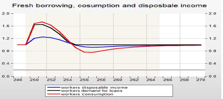
Fig.8
All the figures show the ratio between the “shock scenario” and the “baseline scenario”. Fig. 8 shows the effect of a credit supply shock on workers' consumption and on the stock of debt accumulated in the workers' balance sheets. After the shock workers' consumption jump, reaching its maximum after two periods, then it collapses and falls below the pre-shock level. The recovery takes time and the level of consumption does not return to its pre-shock level in the period taken in consideration. The stock of debt starts to grow after the shock with the consumption. It continues to grow for four periods, then it starts to decline. The consumption dynamics resembles what happened in some
25 Palley “Debt, AD and the Business Cycle: A Model in the Spirit of Kaldor and Minsky,” Journal of Post
27 advanced countries before and after the Great Recession.
Fig. 9
Fig. 9 shows the evolution of the disposable income of workers households with the evolution of the stock of debt. Disposable income starts to grow after the shock as the increase in consumption has an expansionary effect on the economy, increasing the level of income. When consumption starts to decline disposable income declines too. At the same time, the stock of debt grows faster than the disposable income, putting contractionary pressures on the economy.
Fig. 10
Fig 10 shows the movement of demand for loans by workers with consumption and disposable income. After the shock the demand for loans increases following the increases in consumption, when consumption collapses it decline and returns to its pre-shock level.
28
Fig. 11
Fig. 11 shows the effect of the shock on Rentiers’ consumption. Since Rentiers are “low propensity to consume agents”, the expansionary effect of the credit supply shock is small. Figures 9, 10 and 11 illustrate the idea of Kaldor and Palley of the “debt service transfer mechanism”. Debt repayment shifts income from high propensity to consume households to low propensity to consume agents, putting contractionary pressures on the economy.
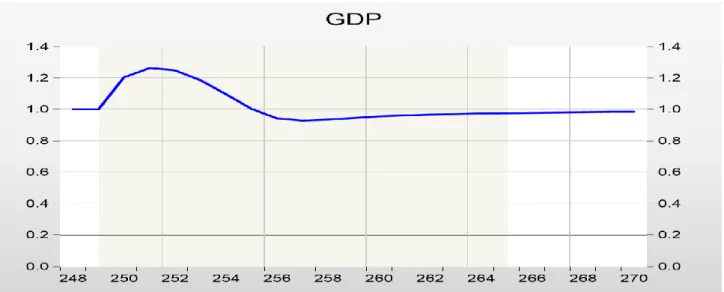
Fig. 12
Fig. 12 shows the impact of the shock on GDP. It increases with consumption and declines when workers cut spending. The “stock-flow” dynamic of inside debt generates a business cycle similar to the one described by Palley: an increase in expenditure financed by borrowing has an expansionary impact on the economy in the first time, when the payback phase begins the “debt service transfer mechanism” puts contractionary forces on the economy.Another interesting result is that recovery from the recession takes time and the economy after the shock is below the “pre-shock” steady-state equilibrium during the number of period considered in this simulation.
29
Fig. 13
Fig. 13 shows the impact of the shock on all the components of the aggregate demand and on the GDP. Workers' consumption is the variable affected directly by the shock. Its recovery is slow and it does not return to the pre-shock level. Investment responds with a lag to the shock and collapse during the consumption-led recession. Investment’s recovery is faster than the recovery of consumption and it returns to the pre-shock level after few periods. This first simulation describes a simple consumption-led cycle in which the economy is driven by workers’ expenditures and the banking’s sector willingness to lend.
6.8) Minskyan extensions
Now, following Palley (1994, 2009) we introduce some extensions in order to study a complete “predator-prey” model of household debt. In this model, the interaction between the impact of borrowing on aggregate demand and on the balance sheets of the borrowers creates a cycle. In order to produce this cycle, we introduce a leverage ceiling to the willingness of the banking sector to lend and to the willingness of the workers to borrow. We assume that once households reach this ceiling, banks reduce the number of loans and workers reduce their demand for credit. The leverage is calculated as the ratio between the stock of debt in the balance sheets and the disposable income of the households. From the Households side, we introduce a different consumption function, similar to the one presented by Palley (1994).
5.1) 𝑆𝐿 = 𝐷𝐿𝑓+ 𝐷𝐿𝑅+ 𝐷𝐿𝑤 ∗ 𝜌
𝜌 = 0.8 𝑖𝑓 𝑙𝑒𝑣𝑒𝑟𝑎𝑔𝑒 < 𝜓
𝜌 = 0.25 𝑖𝑓 𝑙𝑒𝑣𝑒𝑟𝑎𝑔𝑒 > 𝜓
30 the consumption function becomes:
28) 𝑐𝑤 = 𝛼 ∗ 𝑌𝑤𝑑+ 𝐷𝐿 𝑤
We make the assumption that workers households consume all their income plus 𝐷𝐿𝑤. 𝐷𝐿𝑤 is the
demand for loans.
29) 𝐷𝐿𝑤 = 𝜎 ∗ 𝑌𝑤(𝑡−1)𝑑 + 𝜏 ∗ 𝑌̇
30)𝑌̇ = 𝑌𝑤(𝑡−1)𝑑 − 𝑌𝑤(𝑡−2)𝑑
Demand for loans depends positively on the level of income of the previous period and positively by 𝑌̇, this variable captures the: “Minskyian notion of financial tranquillity, whereby periods of income expansion make borrowers and lenders more optimistic, which then enables increased leverage.” (Palley 1994, p. 389)
With these Minskyian extensions, we try to show the “predator-prey” dynamic of debt described by Palley. Fresh borrowing increases aggregate demand and income; this, in turns, increases the ability to borrow more. Fresh borrowing feeds income that feeds back the ability to borrow more. At the same time, fresh borrowing increases the stock of debt in the balance sheets of the borrowers. The increasing level of the stock of debt preys on income by the repayment mechanism.
31
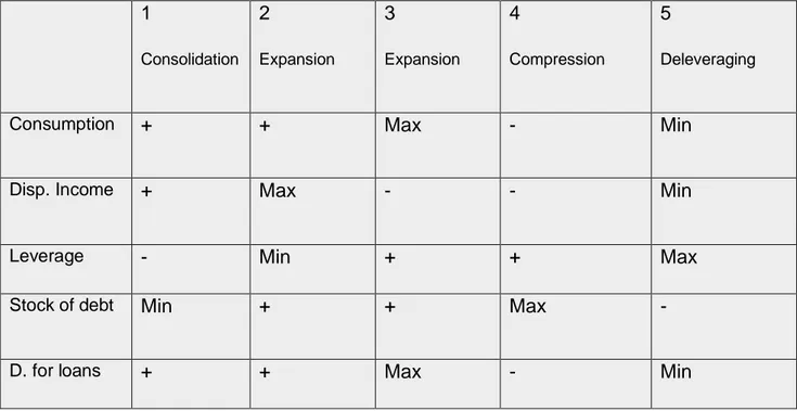
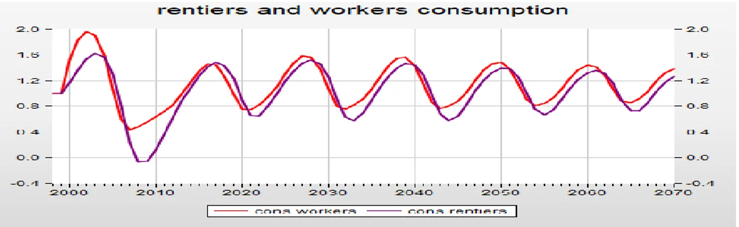
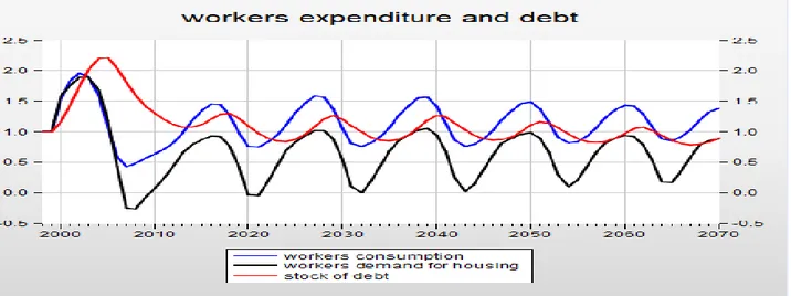
Fig. 15
Fig. 14 and 15 show the predator-prey dynamic described above. As we said above, the economy is hit by a credit supply shock: banks decrease their standard of credit. The difference with the previous simulation is that, in this case there is a leverage ceiling imposed on the borrowers, this means that when the leverage will hit that ceiling the supply of credit will decrease. The interaction between the expansionary and contractionary effect of debt on income in the simulation creates a five-phases cycle that can be easily summarized by the following table
Tab.1 1 Consolidation 2 Expansion 3 Expansion 4 Compression 5 Deleveraging
Consumption + + Max - Min
Disp. Income + Max - - Min
Leverage - Min + + Max
Stock of debt Min + + Max -