Date of publication xxxx 00, 0000, date of current version xxxx 00, 0000. Digital Object Identifier 10.1109/ACCESS.2017.DOI
Fog-Driven Context-Aware Architecture for
Node Discovery and Energy Saving Strategy
for Internet of Things Environments
RICCARDO VENANZI1, (Student Member, IEEE), LUCA FOSCHINI2, (Member, IEEE), PAOLO BELLAVISTA2, (Senior Member, IEEE), BURAK KANTARCI3, (Member, IEEE), and CESARE STEFANELLI1, (Member, IEEE).
1Department of Engineering, University of Ferrara, Via Saragat, 1, Ferrara, Italy (e-mail: [email protected])
2DISI, University of Bologna, Viale Risorgimento, 2, Bologna, Italy (e-mail: [email protected] and [email protected]) 3School of Electrical Engineering and Computer Science, University of Ottawa, Ottawa, Ontario, Canada
Corresponding author: Riccardo Venanzi (e-mail: [email protected]).
ABSTRACT The consolidation of the Fog Computing paradigm and the ever-increasing diffusion of Internet of Things (IoT) and smart objects are paving the way toward new integrated solutions to efficiently provide services via short-mid range wireless connectivity. Being the most of the nodes mobile, the node discovery process assumes a crucial role for service seekers and providers, especially in IoT-fog environments where most of the devices run on battery. This paper proposes an original model and a fog-driven architecture for efficient node discovery in IoT environments. Our novel architecture exploits the location awareness provided by the fog paradigm to significantly reduce the power drain of the default baseline IoT discovery process. To this purpose, we propose a deterministic and competitive adaptive strategy to dynamically adjust our energy-saving techniques by deciding when to switch BLE interfaces ON/OFF based on the expected frequency of node approaching. Finally, the paper presents a thorough performance assessment that confirms the applicability of the proposed solution in several different applications scenarios. This evaluation aims also to highlight the impact of the nodes’ dynamic arrival on discovery process performance.
INDEX TERMS Bluetooth Low Energy, Discovery, Fog Computing, IoT, IoT-Fog Enviroments, Smart Discovery, Power Efficient Discovery, Ski Rental Problem
I. INTRODUCTION
A
DVANCES in wireless communications and mobile devices are enabling new service opportunities and integration possibilities. Internet of Things (IoT) objects are everyday life physical things equipped with computation, storage, communication, and sensing capabilities, such as wearables, sensors, actuators, and even smartphones.Fog computing has a distributed architecture targeting applications and services with widespread deployment as for the IoT [1], [2]. Fog computing is positioned as an interme-diate layer between Cloud computing infrastructure and IoT devices. Thus, fog nodes bridge application objects running in the Cloud and the edge [3], [4]. Fog computing enriches IoT environments with computing resources, communication protocols, location awareness, mobility support, low latency, geo-distribution [5]–[7]. These benefits enhance Quality of Experience (QoE) of IoT applications’ users [8]. Physically, fog nodes are industrial network routers, smart mobile access
points, smart switches deployed into the environments of interest such as smart residential or business buildings, shopping centers, smart urban areas and so on [9], [10]. As a complementing concept to the cloud, fog computing has been identified as a possible solution to ensure energy efficiency at the IoT devices [11]. However, at the application layer, there are still open issues and trade-offs for existing protocols in terms of energy efficiency and reliability of communications [12], [13].
In this paper, we leverage the possibility of easily inte-grating short and medium range wireless connectivity in the same IoT devices to propose novel cross-network management operations to overcome those typical limitations of Bluetooth Low Energy (BLE) discovery [14]. We propose Power Effi-cient Node Discovery (PEND), an enhanced node discovery solution specifically tailored for IoT-Fog environments to ensure sustainability/energy efficiency and discoverability, as well as reliability. The fog layer entity (fog node) bridges
the IoT devices and the Cloud, and provides the needed context awareness about nodes in the locality [15], [16]. Fog nodes (FNs) typically are smart networking appliances equipped with computational and storage capabilities, such as smart access points, smart switches, smart industrial routers, or even powerful smartphones. IoT devices at the edge are considered to be a Bluetooth Low Energy Scanner (BLE-S) and a Bluetooth Low Energy Advertiser (BLE-A) in the subscriber and publisher roles, respectively. The fog node, at fog level, keeps track of the trajectory of the BLE-A, and implements a signaling scheme to control the Bluetooth interface of the BLE-S depending on the geo-location of the BLE-A, which is communicated through WiFi interface. FNs receive BLE-As’ location updates, they store their locations and calculate their trajectory. The signaling scheme allows to synchronize the advertisement and scanning frames leading to 100% discoverability (i.e., Device Matching Ratio–DMR, as used in the paper) of the devices, and remarkable savings in the BLE, CPU, and per-application battery consumption. In addition, in this paper we propose an optimization model, based on the ski rental problem formulation, to save energy by introducing an adaptive BLE interface switching ON/OFF strategy based on the advertisers’ arrival frequency. Finally, we widely assessed the proposed solution and we report a large selection of experimental results that confirm the effectiveness of the proposed solution under different possible configurations by highlighting its advantages and limitations. The remainder of the paper is structured as follows. Section II presents some background material about our research and reports related work. Section III details our proposed model and architecture. Section IV addresses our original solution for adaptive BLE switching ON/OFF strategy with energy saving, while Section V presents experimental results. Finally, Section VI ends the paper and presents our ongoing work directions.
II. RELATED WORKS
BLE has become a strong candidate technology to connect smart objects and IoT nodes [17]–[19]. One of the challenging aspects of the BLE is its discovery process. The BLE discovery phase is critical since it impacts the detection and connection capability of each device. The other main aspect of the discovery phase is its energy efficiency. BLE is particularly tailored for IoT communications and, being the IoT nodes mostly running on battery, the power efficiency has a remarkable importance [20]. Given the above mentioned reasons, BLE discovery and its power efficiency remain open issues and challenges for the researchers in this field.
BLE provides APIs that allow the developers to tune several parameters and settings that impact on the behaviors of the device during the discovery process. The discovery parameters are many. Among the others, the most commonly tuned ones are the scanning frame length, and the scanning interval for the BLE scanner, and the advertising interval, advertising arrival rate, and advertising event duration for the BLE advertiser. By the tuning these parameters, it is possible
to improve the performance of the BLE discovery process [21]. In [22], the authors proposed a discovery approach, named sDiscovery, based on tuning the length of scanning window and scanning interval according to the number of redundant and new devices discovered on each discovery cycle. Redundant devices are devices detected in the current discovery cycle but already discovered in the previous one. In particular, more redundant devices are discovered each cycle, more stable is the environment, and more stable is the environment, more sporadically the discovery process can be scheduled, and the scanning window can be shortened. The approach adopted has two main aspects that can be improved. First, sDiscovery protocol scans the proximity in any case and, then, it checks the number of new devices and adjusts itself. In this way, the protocol scans the proximity even if there are no new devices around. In this case, the protocol tunes the scanning process settings by reducing the frame length and enlarging the scanning interval. Immediately after, new devices might approach and, according with the new scanning adjustment, these new approaching devices might be missed. In a nutshell, the proposed sDiscovery is a good solution in general, but there is room for improvement by aiming the responsiveness of the algorithm. Another possible improvement might be to move the execution of the algorithm for the self-tuning out from the device itself. This might lead to avoid computational overhead.
Another study on tuning the BLE discovery settings in order to improve the discovery process is proposed in [23]. In this article, the authors focus on improving the speed of mass device discovery and prolonging the battery life. In this case, the tuning of the discovery parameters is done at deployment time. This is another good approach, in particular if applied to some specific scenarios. Besides of that, this approach might be improved by addressing the staticity of the discovery process configuration. In this way, it might suit to multiple types of scenario. In [23], conversely from [22], the authors target the tuning of the BLE advertiser by configuring the advertising packet, and the advertising event parameters. The same approach has been adopted in [24]. Here the authors tuned the advertising interval to minimize the discovery time. In this work, the approach adopted by authors is valuable, but it might be improved by making the discovery parameters reconfigurable at run time. An adaptive algorithm might be introduced.
Another valid work in which the authors tuned the advertising settings to improve the discovery process is [25]. In this work, the authors proposed an algorithm to dynamically adjust the advertisement interval considering the network conditions based on a carrier sensing (CS) scheme. This type of approach is valid, in this work the self-adaptive procedure is run directly on the device, and this might cause a CPU and energy overhead. Other previous works, targeting the tuning of advertisement event parameters of discovery process in order to reduce the energy consumption, are [26],
[27]. In these two works there is room for improvements by targeting the same aspects emerged in the previous papers. The first work presents a solution based on a fixed pre-setting of the advertisement parameters. The second one presents a solution based on adaptive strategies, but, also in this case, those algorithms are executed on the device itself. The same drawback emerges also in [28] and [29]. In [28], the authors designed an adaptive strategy to tune the configuration parameters of the discovery process at run time. This strategy aims to adjust both advertiser and scanner settings in order to find the best tradeoff between energy efficiency and responsiveness of the discovery process. In particular, authors aimed to minimize the time needed by the devices to discover each other in the most energy efficient manner possible. Targeting the discovery parameters of the advertiser and scanner is an approach also adopted in [29]. In this work, the authors have developed and adopted a mathematical model which can compute the neighbor discovery latencies for all possible parametrizations. Kindt et al. used such theory for tuning the discovery parameters of scanning and advertising processes in order to improve the device discovery both in terms of power efficiency and discoverability [29].
Complementary to the researches mentioned above, which improve the BLE discovery performance by tuning the dis-covery configuration parameters at a low level, the disdis-covery protocols we designed and proposed in [7], namely PEND and SPEND, exploit the advantages provided by Fog computing. The fog has a pivotal role to exploit the full potential of IoT nodes by enabling the context and location awareness of the nodes. This paper proposes a fog-based architecture aimed to overcome the typical limitations of the conventional discovery approach. The model and architecture, proposed in this paper, aim to optimize the device discoverability and to improve the discovery power sustainability. Our work differs from and complements the previous studies by concentrating on the following original aspects: our solution is not based on any discovery parameters pre-setting, and it does not load the devices with any extra heavy computational algorithm or task. It exploits the support provided by fog to trigger and to configure the discovery process. In this way, all the potentially heavy computational tasks and algorithms are laid on fog nodes, contrary to what the above mentioned solutions have done. Section III presents the system model and corresponding architecture in detail.
In addition, in this article we also propose an energy-saving strategy based on the Ski Rental problem [30]. This type of theoretical problem belongs to the class of problems to help in choosing between a periodic cost, paid repeatedly (rent a pair of skis), and a determined price paid once (buying price). It is demonstrated that the optimal off-line deterministic strategy to minimize losses for this class of problems is to pay the repeated rent cost until it is equal to the buying price, after which, it is better paying the buying cost. We used an
off-line deterministic strategy because this kind of approaches are the simplest and achieve easily reproducible results [31]. The authors in [32], demonstrate that this problem is 2-competitive. This kind of strategy perfectly suits that kind of problem in which there is the dilemma between paying a small amount repeatedly or paying a bigger cost just once, and it has been widely applied [33]–[35].
III. MODEL AND ARCHITECTURE
This section firstly provides a complete overview of the reference model. Then, it introduces the proposed distributed architecture. Finally, the last subsection addresses the pro-posed theoretical energy-saving model based on the "Ski Rental Problem".
A. MODEL
The wide spread of wearables, Body Area Networks (BAN), and Personal Area Networks (PAN) call for new solutions able to efficiently support the continuous connectivity of these smart objects. Bluetooth is the standard de-facto technology for wirelessly connecting any smart device in a short range. This trend has led the research community to focus its attention on the crucial aspects of this technology. In the mobile communication field, one of the hottest topic is the node discovery process. Moreover, speaking of battery-operated mobile nodes, another crucial aspect to address is energy management. The device discovery has a central role in IoT, it enables the nodes connection and the IoT service providing. The Bluetooth Special Interest Group (SIG), with the release of Bluetooth Low Energy (BLE), has paved the way to the massive adoption of Bluetooth as node communication enabling technology in IoT field. BLE is able to provide a quite simple discovery process while keeping the energy consumption relatively low. The applications of BLE discovery-based systems fall in several fields, such as marketing advertisement [36], city’s point of interest discovery [37], sports performance monitoring [38], [39], indoor positioning systems [40], [41], smart health systems [42], just to name few. The traditional or conventional BLE discovery process has a quite simple and trivial architecture, it involves two type of entities, a scanner and an advertiser. The BLE scanner (BLE-S) looks for other devices in the proximity, while the BLE advertiser (BLE-A) announces its presence to the nearby BLE-S. Let us introduce an example of a typical conventional BLE discovery scenario, a BLE beacon is located in proximity of a painting in a museum and it is continuously in the active state scanning the vicinity for other devices. In this scenario, when a new device approaches, it gets discovered and the scanner sends to it all the information about the painting. In this conventional BLE discovery scenario, one of the two entities has a static location and continuously advertises its presence or scans for other devices while, on the other hand, the other entity is supposed to be moving. In this paper, we consider the above described conventional scenario as our reference. In this reference scheme, the BLE-Ss have a static and known position, while
the BLE-As are mobile. In the conventional BLE discovery scenario, the BLE-S constantly and periodically scans for devices in the proximity, being the scan process an endless loop. The other entity of the model, the BLE-A, continuously advertises its presence. As we mentioned before, the BLE-A does not have a static and fixed location, and we assumed it is carried by pedestrian. The BLE discovery process succeeds when an advertising packet sent by BLE-A hits a BLE-S active scanning window. In other words, when an advertising BLE-A is close enough to a scanning BLE-S to allow an advertising packet to hit the BLE-S’s scanning window, the BLE-A is discovered. The conventional BLE discovery approach might result in the following situations: the BLE-Ss keep scanning for devices even if there are no BLE-As nearby, and in the same way, the BLE-As keep advertising their presence even in areas where there are no BLE-Ss. Even in the case in which a BLE-S and a BLE-A are within their discoverable proximity, they might not discover each other. This might occur because the scanning and the advertising process are not synchronized. At low level, a BLE-S scans periodically on three different channels on three different frequencies, namely, 37, 38, and 39, on 2402, 2426, 2480 MHz, respectively. At the same way a BLE-A sends the advertising packets on the same channels (see also [43] for more details on the discovery process works at low level). In this way, for example, if a BLE-A sends an advertising packet on a channel and a BLE-S is scanning on a different one, they do not discover each other. BLE is worldwide used as main short ranged node discovery technology, and it is well known to be power efficient. This does not mean that energy wastage could not still occur, or the BLE discovery process could not be improved. The novel architecture proposed in this work aims to improve BLE discovery process and makes it even more power efficient. We have already introduced the cases in which the conventional BLE discovery scenario results to be not efficient in terms of device discoverability, now we highlight its inefficiency in terms of power consumption. In the conventional BLE dis-covery scenario, the scanners have the BLE interface always active and they scan for devices periodically and constantly, i.e. a BLE beacon. In the same way, the advertisers have also the BLE interface always active and they are in advertising mode, continuously. This approach is clearly inefficient in terms of power consumption. A continuously scanning BLE-S, with no BLE-As around, is wasting energy. In the same way, a BLE-A would significantly save power if it does not advertise its presence in an area where there are no BLE-Ss. Under this point of view, the most power efficient approach would result in the BLE-S and BLE-A enable their BLE interfaces and start scanning/advertising only when they are in the discoverable range of each other. In this paper, we propose a novel architecture that, by exploiting the fog paradigm, aims to overcome the aforementioned issues of conventional BLE discovery scenario. We present an architecture and a new interaction model aimed to heavily improve the BLE device discoverability and BLE energy consumption. The idea is to exploit the characteristics provided by fog computing such
as geo-distribution, location awareness, mobility support and so on, in order to optimize the devices’ discoverability and reduce the power consumption at the same time.
B. DISTRIBUTED ARCHITECTURE
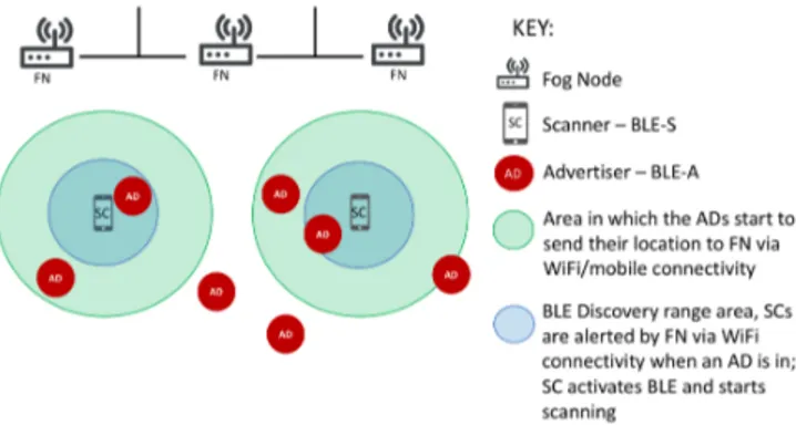
We are proposing a novel architecture for device discovery composed by three entities: BLE Scanner (BLE-S), BLE Advertiser (BLE-A) and Fog Node (FN). We introduced in our model the fog nodes, unlike the conventional BLE discovery scenario, to exploit the advantages provided by the fog paradigm to improve the power efficiency of the BLE discovery process and optimize the devices’ discoverability. Via FNs, we target the discovery synchronization, in other words, we want to make the BLE-Ss and the BLE-As aware of when they are in discoverable proximity of each other, synchronizing the advertising and the scanning process. In this way, the BLE-A and the BLE-S start advertising and scanning only when they effectively are in their BLE range, saving power and optimizing the device discoverability. The architectural model we are going to refer is depicted in Fig.1. We assume the BLE-Ss are located in fixed and static locations, their goal is to discover BLE-As in the most efficient way in terms of power consumption. The BLE-Ss are not connected to any power supply. The BLE-As do not have a static and known position, they are mobile and free to move. We suppose the BLE-As are carried by pedestrians. Their goal is to be discovered and to receive information by the BLE-Ss. The BLE-Ss and BLE-As are smart devices like smartphones. These devices have internet connectivity and a BLE interface. BLE-Ss and BLE-As are connected to FNs via WiFI, over MQTT protocol. The FNs are smart entities connected to the infrastructure, i.e. smart access-points, smart switches, etc. At the beginning, the BLE-As register themselves on FNs. The advertisers subscribe on the topics of the points of interest (POI), in which they are concerned. The FNs load on BLE-As all the POI in where there are BLE-Ss providing the services of interest. For example, recalling the scenario summarized in Section III-A, an advertiser might be interested in some particular artist’s artwork in a museum. More generally, a BLE-A might be interested in some selected commercial advertising, food or drink spots, some touristic attractions, therefore any type of POI with location-based service. In this way, only a restricted set of BLE-Ss are loaded to the BLE-A and it will not be involved in the discovery process by each nearby BLE-S. When a BLE-A enters in one of the pre-fetched POI’s areas (green areas in Fig.1), it starts sending its location to the FNs. In this way, the FNs become aware about BLE-As position. When a BLE-A enters in the BLE discovery range of a BLE-S (blue areas in Fig.1), the FN alerts that specific BLE-S and makes the discovery process synchronized and starting. When a BLE-S is alerted by a FN, it switches the BLE interface to ON and begins the scanning process, at the same time, the BLE-A begins the advertising process, in a fully synchronized manner. In this way, we optimize the BLE device discoverability, activate BLE interface and discovery process only when it is strictly needed, and reduce the power
FIGURE 1: The architectural model of our presented scenario. .
consumption. Our model leverages the awareness given by fog paradigm in order to optimize the device discoverability and minimize the scanner power consumption at the same time. The model depicted in Fig. 1 describes a three entities architecture composed by BLE-Ss, BLE-As, and FNs. The communication between the FNs and BLE-S/A are via MQTT over WiFi connection. The WiFi connectivity of the IoT nodes (BLE-Ss and BLE-As) does not significantly impact on the power consumption because WiFi interactions are few, and the interface is mostly in idle state. Moreover, the interactions are over MQTT, a widely recognized lightweight protocol with extremely low energy impact. The architecture presented is focused on improving the conventional BLE discovery scenario described in Section III-A, primarily in terms of device discoverability, and then in terms of energy sustainability. This goal is achieved by the introduction and the exploitation of FNs. In our model architecture, we use the WiFi connectivity only for the few interactions among IoT nodes and FNs, while the most onerous operations, such as discovery process, are running on BLE. In this way, we achieve the BLE discovery process optimization, besides keeping the energy consumption as low as possible. Contrary, by using the WiFi connectivity even for the discovery part, the model would lose its core concept of locality provided by BLE technology. This occurs because, as it is widely known, WiFi is long-ranged communication technology with ranges reaching to 200 meters whereas the BLE reach is at the order of a few meters. With this size of range an advertiser could receive information regarding a multitude of POI, and not only from the nearest one. This causes the loss of the proximity interest concept. Recalling the museum example above, an advertiser would receive information from most part of the artworks in the museum, while the visitor would be only interested the artwork in front of him/her or, in any case, in his/her closest proximity. With the latter version, BLE gives the possibility to extend its range up to longer distances, a few tens of meters [44]. However, this extension cannot reach the distance coverable by WiFi technology. BLE is still a short range communication technology, and it perfectly fits our concept of locality.
The proposed architectural model has two components
of power consumption: the BLE activities and the WiFi connection. As it is stated before, the discovery-related activities are the most onerous in terms of power consumption. These operations are performed on BLE technology. Hence, firstly, we focused on reducing the power consumption of the BLE discovery process. At this first stage, we kept the WiFi connectivity of the scanner always active, targeting the power consumed by BLE usage. The BLE interfaces of BLE-Ss are kept OFF at the beginning. In the proposed model, the BLE-As are in permanent movement and, as soon as a BLE-A enters in the BLE-S’s POI area (green area), it starts sending its location and its UUID to the FN via MQTT, making the FN aware about the position of the advertiser and its ID. When the BLE-A gets closer to BLE-S, in the BLE discovery range (the blue area), the FN alerts the relative BLE-S that switches on its BLE interface and starts scanning for that specific BLE-A. The FNs, being aware of the location of the BLE-Ss and BLE-As, alert and wake up the BLE-S only when the BLE-A is in the BLE range. This synchronization makes the device discoverability guaranteed, minimizing the active time of the BLE interface. Once the BLE-A is discovered, the BLE in-terface will be switched OFF. It is easily understandable that, according with the approach aforementioned, the switching ON/OFF of the BLE interface is strictly dependent by the arrival of BLE-As. This kind of interaction protocol and its improvement have already been described as Power Efficient Node Discovery (PEND) and Smart PEND (SPEND). A deeper and more accurate description and analysis of these two protocols can be found in [45]. The aforementioned protocols have been proved to be a remarkable improvement of the conventional BLE discovery scenario, in which the fog paradigm is not involved, in terms of power efficiency. In the previous work, the focus was mainly laid on the interaction between BLE-A and BLE-S. In this work, we propose a new strategy for the cost optimization in terms of power consumption. We aim to reduce the power consumption further and show new original unpublished experimental results.
In the model already presented the BLE interface usage is reduced but the WiFi connectivity is always active. In order to improve even more the power saving, we tried to reduce also the WiFi connectivity usage. The problem is addressed by keeping the WiFi interface OFF at the beginning, and setting a timer on BLE-Ss. When the timer triggers the BLE-S connects to the FN, and if there are BLE-As in the proximity, it activates the BLE interface and it starts scanning for devices. The FN, being aware of the BLE-As’ location and their speed, sets up the next timer value. The disadvantage of this kind of approach is that the model might not guarantee the discoverability of a BLE-A. Indeed, with a bad setting of the wake-up timer on BLE-S, a BLE-A might pass through the BLE-S’s area without being discovered. This kind of approach paves the way to several challenges, for instance, what is the minimum value of the timer that guarantees the discoverability of the BLE-As? And then, which is the best trade-off between losing some BLE-As and saving more power?
In the next section a deep analysis regarding a switching ON/OFF strategy to minimize the power consumption for the first stage of the model will be presented. Furthermore, we face the calculation of the minimum wakeup timer of the BLE-Ss for avoiding the advertisers’ losses.
IV. ADAPTIVE BLE SWITCHING ON/OFF STRATEGY FOR ENERGY SAVING
Originally, in the conventional BLE discovery approach, described in Section III, the BLE interface of BLE-S was kept always in ON state, and the scanning process was performed constantly and periodically at a fixed rate. Then, with the architecture we proposed and the protocols we introduced in [45], the switching ON/OFF of the BLE interface, and the activation of the scanning process are triggered by FNs. According to our approach, the ON/OFF switching of the BLE-Ss’ BLE interface and the activation of the scanning processes became dependent by the arrival of the BLE-As. Hence this approach, is strongly dependent by the BLE-As’ arrival rate. Consequently, if the BLE-A’s arrival rate significantly grows, the number of times that a BLE-S has to switch ON/OFF the BLE interfece and perform a the scanning process, grows as well. In this case, the BLE-S might enter a continuous BLE switching ON/OFF status. This kind of status results in higher power consumption than keeping the BLE always active (conventional BLE discovery scenario).
With a high arrival rate of the BLE-As, it might be more power efficient to keep the BLE interface of the BLE-S always active, with periodic scans. This falls in a balance dilemma between switching continuously ON/OFF the BLE interface or adopting the conventional strategy, keeping the interface always active. The balance dilemma just described belongs to class of problems of choosing between paying a periodic cost (rent a pair of skis) or paying a bigger cost just once (buying price). This class of problems is known as ’Ski Rental problem’ [46]. The best off-line deterministic strategy is paying the rental cost until the accumulated expense does not reach the buying cost, then, it is better paying the buying cost instead. In our model, it means that the optimal strategy in term of power saving is to adopt the strategy of switching ON/OFF the BLE interface of the scanners at every BLE-A’s arrival until the power consumption due to continuous switching becomes equal to keep the interface always active. We address the problem only in terms of power consumption, assuming the scanning frequency of the conventional scenario high enough to avoid the device discoverability losses. This strategy belongs to the class of two-competitive algorithms in which the optimum is given by the ratio between the buying cost over the rental price. More formally, the proposed analysis is based on two metrics; Energy of SWitching (ESW) is the energy consumed for switching on the BLE interface, the energy required for the scanning process, and the energy required to switch off the interface. The sum of these three elements has to be repeated each time a BLE-A enters in the BLE discoverability range, plus the energy consumed by keeping the WiFi connectivity active and the MQTT activities
(low). ESW is namely the repeating cost of renting. The Energy UP (EUP) is the energy consumed by keeping the BLE interface always active with a periodic scan process, it is the energy consumed by adopting the conventional BLE discovery approach. It is given by the sum of the energy consumed by switching on and off the interface just once (at the beginning and at the end), plus the energy consumed by the scanning process multiplied for the scanning frequency. The scanning frequency is supposed to be static and calculated over a finite period of time, significantly larger of a single scanning window, i.e. one hour. EUP is namely the buying cost of the ski. Formally the two metrics are expressed in the Equation 1a and 1b E SW= ewi f i+ N Õ i=1 (eO N i+ eOF F i+ eSC AN i) ∗ f rARRi∗δi (1a) EUP= eO N + eOF F+ eM AN+ (eSC AN∗ f rSC AN) (1b) Where N is total number of BLE-As in the system, eONand eOFF are the energies required to activate and deactivate the
BLE interface, respectively. The eMANis the energy required
to keep the interface active, while eSCANrepresents the energy
consumed by the scanning process. Furthermore, let ewifibe
the energy consumed by keeping the WiFi connectivity always active and the MQTT activities. Then, frSCANand frARR are
respectively the scanning frequency of a BLE-S and the arrival frequency of the BLE-As. While δiis a boolean variable, it is
1, if the ith A is in the BLE discovery range of a
BLE-S, 0 otherwise. Once we have defined the aforementioned metrics, we can obtain the optimum of our balance dilemma. The optimum, according with the deterministic 2-competitive strategy for this class of problem, is given by the division of EUP over ESW. The optimum in our case is meant as the maximum number switching ON/OFF of the BLE interface before adopting an always active conventional-like strategy results to be more power efficient. The optimum OPT is calculated with the Formula 2a, then Formula 2b.
OPT= EUP E SW
= eO N + eOF F+ eM AN+ (eSC AN∗ f rSC AN)
ewi f i+ ÍNi=1(eO N i+ eOF F i+ eSC AN i) ∗ f rARRi∗δi
(2a) considering the worst case in which every BLE-A enters in the BLE discoverability range and defining eSWas (eON+ eOFF),
equation 2 becomes:
= eSW + eM AN+ (eSC AN∗ f rSC AN)
ewi f i+ [(eSW+ eSC AN) ∗ N ∗ f rARR] (2b)
As already stated, considering a finite period of time T,
optimum totally dependent by frARR.
The second power consumption component of our system is given by the WiFi connectivity always active. We tackle this aspect by turning the WiFi connectivity of the BLE-Ss in OFF state for a certain period of time. The timer that wakes up the connectivity of the BLE-Ss is driven by FNs. The BLE-As start to send their location as soon as they enter in a BLE-S’s POI area (green area), making the FNs aware about their ID and location. With the BLE-A’s location constantly updated, the FNs are able to calculate the advertiser’s speed and arrival frequency. The FNs, are smart infrastructural appliances, equipped computational and storage capabilities. Though the continuous update of the BLE-A’s location (in green area), the FN can calculate the BLE-A’s speed and its arrival rate, supposing that constant. Given all those information, the FNs are capable to efficiently set a wakeup timer on the BLE-Ss. With the WiFi connectivity not always active, the device discovery is not guaranteed. With the WiFi connectivity in OFF state, the FN would not be able to alert the BLE-S of an approaching BLE-A, and, in this case, the advertiser would not be discovered. It is necessary to find a trade-off between power saving and device discoverability. This is a wide problem with multiple solutions, and each of them is strictly dependent by the application context. We approach the problem by calculating the minimum timeout that guarantees the discoverability of all BLE-As.
We assume the museum context cited in the example used in previous sections. The BLE-Ss are placed on points of interest (specific art works), and they have a circular area of radius r as BLE discoverability range. In addition, as it has already stated, the BLE-As are devices carried by pedestrians with a certain reduced speed (VBLE-A, supposed constant) and
an arrival frequency (frARR). It is reasonable to state that the
minimum wakeup period of the BLE-Ss must be less than the BLE-A’s arrival period plus the time the BLE-A takes to entirely across the BLE discoverability area (blue area) of the BLE-S (tAREA). Formally this relation is expressed in the
Formula 3a, 3b, and 3c:
TW AK EU P< TARR+ tARE A tARE A= 2 ∗ r VBLE− A (3a) => TW AK EU P< TARR+ 2 ∗ r VBLE− A (3b) => f rW AK EU P> 1 TARR+VB L E − A2∗r (3c)
Where TW AK EU Pis the wakeup period of the BLE-S, TARR
is the BLE-A arrival period, and tARE Ais the time needed to
completely across the whole BLE discovery area. Assuming the speed of the BLE-As known and constant, the frWAKEUP
becomes dependent by frARR. The FNs are aware of
BLE-A’s speed and the radius of the area, and according with the historical of the arrival frequency of the BLE-As, the FNs
are capable to estimate and set the wakeup timeout on the BLE-Ss.
V. EXPERIMENTAL RESULTS
In the previous section we have underlined how the impact of the advertisers’ dinamicity is crucial for the performance of our model and, more widely, for the device discovery process in general. In this section, we give a practical aspect to the energy saving strategy presented in the previous section. We study more in detail the relation between EUP and ESW and how this latter varies according to the BLE-A’s dynamic arrival. We have implemented the Formula 2b, and we are going to discuss all its aspects. We have highlighted how the impact of dinamicity of advertisers’ arrival is crucial in our model, in the last subsection we applied the BLE-A arrival dynamicity to PEND and SPEND protocols comparing them with the conventional device discovery scenario running on the presented architecture. As we have already stated, our model exploits PEND and SPEND as device discovery pro-tocols. These protocols have already been introduced in [45], with preliminary results and a study of their performance. We widely extended the experiments presented in our previous work by introducing the dynamic arrival of the BLE-A and a study on how the performance are affected by the dinamicity of the BLE-As. We present and discuss the novel results regarding PEND and SPEND. In these new experiments, we have combined the impact of advertiser arrival dinamicity with the different lengths of BLE-S scanning window.
ENERGY SAVING STRATEGY IMPLEMENTATION
In this subsection, we present a study based on the proposed energy saving strategy due to the implementation of the Equation 2. We estimated all the parameters from the ex-periments run on Conventional scenario, PEND and SPEND, then, we applied them to the equation. We calculated the theoretical maximum number of BLE interface ON/OFF switching before a smart interface switching approach turns to be more power inefficient than Conventional scenario. We also analyzed and plotted how this number change by varying the frequency of BLE-A’s arrival. The data used for implementing the Equation 2b has been calculated by the experiments run on PEND, and Conventional scenario, these data is summarized in Table 1.
TABLE 1: Parameters values of the optimal number of switching equation.
Parameter Value
EUP 43,5 [mAh]
ewifi 3,25 [mAh]
esw+ eSCAN 0,48 [mAh]
N {20, 30, 40, 50}
EUP is the energy of keeping the BLE interface constantly ON and in periodic scanning. It is the energy consumption that reflects the scanner behavior under the Conventional scenario.
FIGURE 2: Ratio between EUP and ESW. It results in the optimal number of ON/OFF switching of the scanner’s BLE interface according with 2-competitive strategy applied to our model.
.
Briefly, we statically tuned the BLE-S’s scanning frequency and scanning frame length by setting the inter-scanning period to 30 seconds, and the frame length to 30 seconds. By doing so, we focus our attention on BLE-A’s arrival, and we make the equation strictly dependent by advertiser’s arrival frequency. Once the scanning frequency is defined as static, EUP becomes a constant and its value can be easily fetched by Conventional scenario experiments. The other values of the parameters has been fetched by the energy consumption report made by the Android Device Bridge during the experiments [47]. The values are calibrated on experiment with a finite time duration of 60 minutes. We needed a experimental duration long enough to let us run the discovery process several times. Since the single process duration goes from 10 seconds up to 60 seconds, we picked one hour as single run duration. The whole set of the experiment settings is listed in Table 2. It is worth to note that EUP represents the power consumption of the Conventional discovery scheme. Its value in Table 1 has been calculated from the experiment with a scanning frame length of 30 seconds, scanning period of 30 seconds, advertiser arrival period of 60 seconds and advertising frame length of 30 seconds. The energy consumption due to WiFi interface utilization is expressed with ewifi, while esw+ eSCAN
is the energy consumed by a single switching ON/OFF of the BLE interface plus the energy due to the scanning process. N is the number of the total advertisers in the system. Fig. 2 depicts the ration between EUP and ESW on varying of the BLE-A’s arrival period. We plotted four trends changing the total number of BLE-As in the system, N.
The chart in Fig. 2 shows how the number of optimal switching varies according with the arrival of the BLE-As. We implement the proposed strategy with four different number of total advertiser devices within the whole system. The values of N used are, 20, 30, 40, 50 devices. On the X axis there are the values of the advertiser arrival period, expressed in
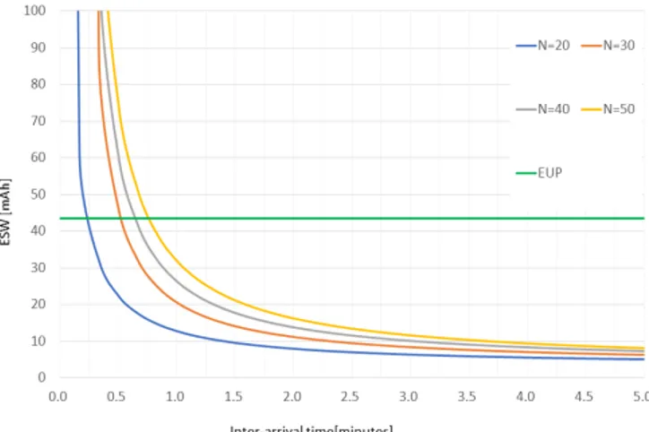
FIGURE 3: Energy values of EUP and ESW in relation with the BLE-A arrival period.
.
minutes, while the Y axis represent the optimal number of ON/OFF switching. From the chart in Fig. 2 emerges the ratio between EUP and ESW has an asymptotic trend. This behavior is reasonable because with the enlarging of the arrival period, the BLE-A arrives ever more sporadically. With a such very occasional arrival, the BLE-S basically, does not ever switch ON its BLE interface, and the ewifibecomes the
predominant component of the ESW. If we push the arrival period to the infinite, the energy consumption of the BLE interface becomes 0, because the BLE-S never switches the BLE interface ON, and the ratio between EUP and ESW turns to be a fraction of two constant value. The value of the asymptote is the result of outcoming division. On the other hand, with a BLE-A’s arrival period close to zero, hence with an arrival frequency very high, the number of time of BLE interface ON/OFF switching drastically drops to zero. This because, under an high BLE-A arrival rate, it would be much more power efficient to keep the BLE interface always ON and scanning. In the chart depicted in Fig. 3, we put in relation the energy values of our two component, EUP, and ESW, with the BLE-As’ arrival period.
Also in Fig. 3, we plot the trends of ESW under the same four different number of total devices as before, 20, 30, 40, 50. In addition, in this chart, we also plot the behavior of EUP. This trend has a constant value because, by definition, it is not affected by BLE-A’s arrival. On the other hand, the trends referring to ESW are strongly dependent by advertisers’ dinamicity. Indeed, from the Fig. 3, clearly emerges how the energy consumption varies according with the arrival period. The ESW component has a asymptotic behavior. Indeed, with the enlarging of arrival period, the BLE-S using the BLE interface switching strategy consumes ever less. If we push the BLE-As’ arrival period to infinite the trends of ESW result to be 3,25, the value of energy consumed by the WiFi usage. This is reasonable because with an infinite arrival period, hence an arrival frequency equal to zero, the BLE-As result
to be never approaching, hence, the component of energy consumption due to the BLE interface usage is 0, and the ESW results to be ewifi. In the opposite case, with a very
little arrival period, hence with an arrival frequency high, the energy consumption due to the switching strategy results to be extremely high. Under this condition applying the strategy of keeping the BLE interface always ON and in periodic scanning would result much more power efficient. According with what we have already stated so far, a question might be risen, what is the advertiser’s threshold arrival frequency after which is better to switch from a BLE interface switching strategy to a BLE interface static one? It is worthy to be highlighted that the EUP straight line intersects the curves of the ESW trends in a point. The value of projection of that point on the X axis is the threshold arrival period, hence the threshold arrival frequency can be easily obtained.
THE IMPACT OF ADVERTISERS’ DINAMICITY ON PEND AND SPEND
We have already mentioned along the whole paper the crucial role of BLE-As dynamic arrival in our model. The architecture introduced in this paper exploits PEND and SPEND protocols. These mechanisms have been already presented in IEEE ICC 2018 conference [45], and, in this manuscript, we extend the our previous work introducing a novel study about the impact of BLE-As arrival dinamicity on these protocols. In this subsection we present a set of new experiment runs, that combine the impact of dynamic arrival of advertisers and the different lengths of the scanning frame. We firstly present the impact of the BLE-A dynamic arrival on the Device Matching Ratio (DMR) and then on the power consumption. It is worthy to be reminded the definition of DMR. The Device Matching Ratio, DMR, is defined as the percentage of the scanning windows in which at least an BLE-A has been discovered out of the total number of scanning windows within a limited period of time, [45]. As we have done in the previous work, we study the performance of Conventional, PEND and SPEND schemes by varying the advertiser arrival rate according the Poisson distribution, over three different scanning frame length. We scheduled the BLE-A’s arrival with an average rate of λ. Thus, the inter-arrival times between two consecutive advertisers would follow the negative exponential distribution with the mean β= 1/λ. In the experiments, we vary the inter-arrival time (β) within the following set {30s, 60s, 90s, 120s}, while the scanning frame length within this other one {10s, 30s, 60s}. It is worthy to remind that, SPEND deactivates the scanning frame immediately upon the detection of a device match. Therefore, SPEND is not affected by the frame length in the experiments. Table 2 presents the details of the experimental settings. According with the approach used in the our previous work, the performance study regarding the energy consumption is broken down into the following components: 1) Battery drained by BLE interface of the BLE-S, 2) Battery drained by CPU as a result of BLE-initiated processes, and 3) Battery drained by CPU accounted to the discovery application process.
TABLE 2: General and discovery strategy-specific settings in our experiments.
Parameter Value
Node Discovery Schemes Conventional, PEND, SPEND
BLE-A and BLE-S operating systems Android 6.0.1 Marshmallow Number of experiments per scenario 12
Total number of runs per experiment 30 Duration of a single run 60 minutes BLE-S Scanning Frame Length {10, 30, 60} sec. BLE-A Advertising Frame Length (`) 30 sec.
BLE-A Inter-arrival duration scheduled according to Pois-son Distribution
Inter-arrival time β 1/λ
(β) values for Poisson Distribution {30, 60, 90, 120} sec. MQTT Broker Type Mosquitto Server BLE Activity in Conventional Discovery Always Active BLE Activity in PEND MQTT Broker-Triggered BLE Activity in SPEND MQTT Broker-Triggered BLE-S Scanning Frame Rate in
Conven-tional Discovery
1 every 30 sec. BLE-S Scanning Frame Rate in
PEND/SPEND
On demand
The following charts shows the trend of DMR under Conventional, PEND and SPEND by varying the frame length of the BLE-S. Fig. 4 depicts four different series, one for each β according the parameter listed in Table 2.
FIGURE 4: Device Match Ratio of Conventional, PEND and SPEND over the different BLE-S’s frame lengths. The series depicted in the chart represent the affection of different β on the DMR of Conventional, PEND and SPEND. The DMR of PEND and SPEND is not influenced by the dynamic arrival of BLE-As since they activate the BLE interface and the scanning process if and only if there is a discoverable BLE-A. Thus there is just one trend attributed to PEND/SPEND.
In Fig. 4 is depicted the DMR behavior of the three schemes under varying arrival rates (i.e. inter-arrival times, β) of
BLE-A and the BLE-S scanning frame length. BLE-As seen in Fig. 4, the PEND/SPEND schemes are represented by only one line, this happens because the scanning process under these two approaches is triggered by the fog nodes any time a new BLE-A approaches. This policy guarantees the discoverability of the BLE-A, hence the DMR is 100% under any BLE-A arrival rate. On the other hand, in the Conventional scenario, the scanning process is constant and periodic, hence the DMR is strongly dependent by the BLE-A’s arrival. From Fig. 4 is easy to observe how the DMR of the Conventional increases with the enlarging of the frame length. On the BLE-A arrival rate side, the DMR decreases as the inter-arrival (β) time grows. From the Fig. 4 emerges that in case of advertisers’ arrival rate reasonable high, i.e. β = 30 sec., and a scanner’s frame length large enough, i.e. 60 sec., the DMR performance of the Conventional scheme might reach a performance close to the PEND/SPEND one; As a side effect, it can drive to massive battery consumption. On the other hand, when the advertisers’ inter-arrival time grows, the DMR performance of Conventional scheme significantly decrease down to less than 20%, in case of λ = 120 sec, and BLE-S’ scanning frame length 10 seconds.
We studied the power consumption of the BLE under a scanning frame length of 10, 30 and 60 seconds and by setting β, the advertiser inter-arrival time, to 30, 60, 90, and 120 seconds. From Fig 5 emerges how, under Conventional scheme, the power consumption decreases as the scanning frame length gets longer. While the trend of the power consumption grows with the enlarging of the scanning windows under PEND. On the other hand, PEND scheme takes advantage form fog node awareness and the BLE-S’s scanning process is activated only when a device is in discovery range, hence it also guarantees the discovery of new device. Under this assumption, it is reasonable to state that PEND does not need to have a long frame length. With a high BLE-A arrival rate (β = 30 s), the power drained under PEND increases accordingly with the increasing of frame length. It becomes greater than the energy drained under Conventional. This because, under PEND scheme, with our experiments settings, a high arrival rate combined with a large frame length leads the BLE-S to be always ON with the scanning process always active. The Conventional scheme is not advertiser’s arrival dependent, hence, it is not affected by the arrival rate. This means that, if the advertisers’ arrival rate is very high, it might be better to adopt a Conventional-like strategy instead of PEND-like one in terms of power efficiency. The dependency of PEND/SPEND from the advertisers’ arrival leads the proposed schemes to have better performance in term of power consumption as the time between two consecutive arrivals (β) increases. On the other hand, the Conventional scheme is arrival independent, hence the power consumption is about constant under different β. SPEND shuts immediately down the scanning process and the BLE interface after the discovery of the new device, it does not wait for the entire frame length. This behavior makes the scheme independent by the different scanning frame lengths. SPEND results to have
(a) BLE power drain with a scanning frame length of 10 seconds, under different inter-arrival time.
(b) BLE power drain with a scanning frame length of 30 seconds, under different inter-arrival time.
(c) BLE power drain with a scanning frame length of 60 seconds, under different inter-arrival time.
FIGURE 5: BLE power consumption under different scanning frame lengths and advertiser’s inter-arrival times.
the best performance in terms of power consumption under every condition, it also guarantees the device discoverability. In the next figure (Fig. 6) is depicted the power drained by the CPU due to the BLE usage.
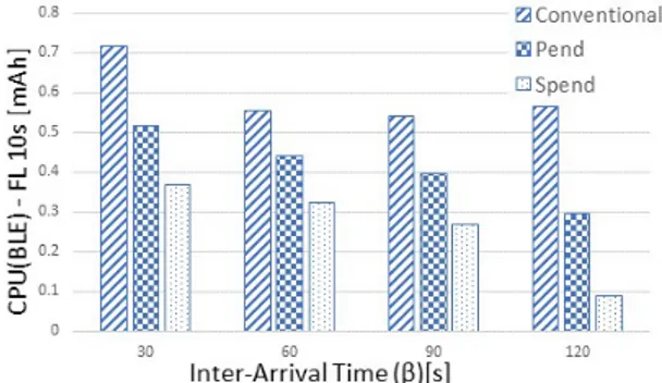
Fig. 6 shows the broken down charts of the power drained by the CPU due to the BLE interface usage. The charts represent the power consumed by varying the arrival time between two consecutive BLE-As (β) from 30 up to 120 seconds in average. The three charts relates the power consumption just
(a) CPU power drain due to Bluetooth activity with a scanning frame length of 10 seconds, under different inter-arrival time.
(b) CPU power drain due to Bluetooth activity with a scanning frame length of 30 seconds, under different inter-arrival time.
(c) CPU power drain due to Bluetooth activity with a scanning frame length of 60 seconds, under different inter-arrival time.
FIGURE 6: CPU power drain due to Bluetooth activity under different scanning frame length and advertiser’s inter-arrival time.
described with different values of β on changing of the BLE-S’s scanning frame length, 10, 30, 60 seconds in, 6a, 6b, and 6c respectively. Fig. 6 highlights how the power consumption generally grows as the BLE-S’s scanning window enlarges. One of the impact factors of this consumption is the number of scanning cycles on the three different frequency channels during the scanning process. In fact, when the scanning
process is active, the BLE interface constantly scans three channels on three different frequencies, namely 37, 38, and 39 (2402, 2426, and 2480 MHz). Hence, it is understandable that larger is the scanning frame length, higher is the number of cycles per window. We got the worst case under PEND scheme with frame length 60 seconds and inter-arrival time 30 seconds. It is worthy to remind that the scanning process under PEND is BLE-A’s arrival dependent and MQTT-triggered. With a large scanning window and an arrival rate high enough, the BLE-S’s scanning process would be always active. On the other hand, Conventional scenario is not arrival dependent and the consumption under this scheme is driven by the number of times BLE-S discovers a new device. Finally, SPEND is proved to be the best scheme even under this aspect. As the other experiments, it is not affected by the window’s length, and thanks to its policy of shutting down the scanning process as soon as a new device is discovered, SPEND has very low power consumption. The energy drained is low also because SPEND discovers the new device very probably at the first scanning cycle, then it stops the scanning process, hence, the consumption of energy is kept as low as possible. In the next figure, the energy consumption due to CPU usage by the application is depicted.
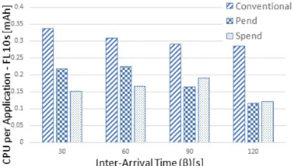
The charts in Fig. 7 depict the power consumed by the CPU of whole application under different settings of BLE-S’s scanning frame length and BLE-A’s inter-arrival time. It is worthy to be highlighted that the CPU power consumption depicted in this figure, represents only the power consumption of the CPU accounted to the application process, and it does not account the BLE part. Fig. 6 accounts the power CPU consumption due to BLE utilization, and it is aggregated into BLE power consumption. Generally, the trend of CPU power consumption of the whole application follows the BLE’s one. It increases as the scanning frame gets larger under each scheme. From Fig. 7 emerges that the Conventional scenario typically has an higher power consumption than PEND and SPEND.
VI. CONCLUSIONS AND FUTURE WORK
The introduction of fog-layer coordination in IoT device discovery can significantly help in improving device dis-coverability and in increasing power sustainability. The fog paradigm enhances the IoT capabilities acting as a mid-dleware between IoT nodes and Cloud. Fog supports IoT environments by providing location awareness, computing resources, mobility support, geo-distribution, and so on. These features are crucial for improving the quality of experience and the efficiency of service providing and seeking in IoT environments.
The architecture presented in this work exploits the fog paradigm to improve the BLE node discovery in terms of device discoverability and in terms of power consumption. Our model, leveraging the location awareness of the nodes in the proximity, effectively triggers the discovery process thus granting PEND/SPEND full discoverability by overcoming typical issues of the conventional BLE discovery. At the
(a) CPU power consumption of the whole application. It run with a scanning frame length of 10 seconds, under different inter-arrival time.
(b) CPU power consumption of the whole application. It run with a scanning frame length of 30 seconds, under different inter-arrival time.
(c) CPU power consumption of the whole application. It run with a scanning frame length of 60 seconds, under different inter-arrival time.
FIGURE 7: CPU power consumption of the whole appli-cation. with different BLE-S’s scanning frame length and varying the BLE-A’s inter-arrival time.
same time, the employed ski-rental optimization allows to save energy by self-adapting the discovery process.
Boosted by these significant results, we are already working on two main future work directions. On the one hand, we are implementing real mobility patters for the advertisers in order to have a much more realistic feedback on the performance of our model. On the other hand, we target to develop a new probabilistic technique based on machine learning algorithms
to nowcast short term user mobility so to further improve the energy saving strategy.
REFERENCES
[1] O. Osanaiye, S. Chen, Z. Yan, R. Lu, K. K. R. Choo, and M. Dlodlo, “From cloud to fog computing: A review and a conceptual live vm migration framework,” IEEE Access, vol. 5, pp. 8284–8300, April 2017.
[2] A. Dastjerdi, H. Gupta, R. Calheiros, S. Ghosh, and R. Buyya, “Chapter 4 - fog computing: principles, architectures, andapplications,” in Internet of Things, R. Buyya and A. V. Dastjerdi, Eds. Morgan Kaufmann, 2016, pp. 61 – 75. [Online]. Available: http://www.sciencedirect.com/science/article/pii/B9780128053959000046 [3] M. Aazam and E. Huh, “Fog computing and smart gateway based communication for cloud of things,” in 2014 International Conference on Future Internet of Things and Cloud, Aug 2014, pp. 464–470.
[4] F. Bonomi, R. Milito, J. Zhu, and S. Addepalli, “Fog computing and its role in the internet of things,” in Proceedings of the First Edition of the MCC Workshop on Mobile Cloud Computing, ser. MCC ’12. New York, NY, USA: ACM, 2012, pp. 13–16. [Online]. Available: http://doi.acm.org/10.1145/2342509.2342513
[5] M. Chiang and T. Zhang, “Fog and iot: An overview of research opportunities,” IEEE Internet of Things Journal, vol. 3, no. 6, pp. 854– 864, Dec 2016.
[6] M. Yannuzzi, R. Milito, R. Serral-Gracià, D. Montero, and M. Nemirovsky, “Key ingredients in an iot recipe: Fog computing, cloud computing, and more fog computing,” in 2014 IEEE 19th International Workshop on Computer Aided Modeling and Design of Communication Links and Networks (CAMAD), Dec 2014, pp. 325–329.
[7] A. V. Dastjerdi and R. Buyya, “Fog computing: Helping the internet of things realize its potential,” Computer, vol. 49, no. 8, pp. 112–116, Aug 2016.
[8] W. Wang, Q. Wang, and K. Sohraby, “Multimedia sensing as a service (msaas): Exploring resource saving potentials of at cloud-edge iot and fogs,” IEEE Internet of Things Journal, vol. 4, no. 2, pp. 487–495, April 2017.
[9] A. Majd, G. Sahebi, M. Daneshtalab, J. Plosila, and H. Tenhunen, “Hierarchal placement of smart mobile access points in wireless sensor networks using fog computing,” in 2017 25th Euromicro International Conference on Parallel, Distributed and Network-based Processing (PDP), March 2017, pp. 176–180.
[10] C. Chang, M. Liyanage, S. Soo, and S. N. Srirama, “Fog computing as a resource-aware enhancement for vicinal mobile mesh social networking,” in 2017 IEEE 31st International Conference on Advanced Information Networking and Applications (AINA), March 2017, pp. 894–901. [11] F. Jalali, S. Khodadustan, C. Gray, K. Hinton, and F. Suits, “Greening
iot with fog: A survey,” in 2017 IEEE International Conference on Edge Computing (EDGE), June 2017, pp. 25–31.
[12] S. Sarkar and S. Misra, “From micro to nano: The evolution of wireless sensor-based health care,” IEEE Pulse, vol. 7, no. 1, pp. 21–25, Jan 2016. [13] F. Jalali, K. Hinton, R. Ayre, T. Alpcan, and R. S. Tucker, “Fog computing
may help to save energy in cloud computing,” IEEE Journal on Selected Areas in Communications, vol. 34, no. 5, pp. 1728–1739, May 2016. [14] F. Zhu, M. W. Mutka, and L. M. Ni, “Service discovery in pervasive
computing environments,” IEEE Pervasive computing, no. 4, pp. 81–90, 2005.
[15] M. Aazam and E. Huh, “Fog computing: The cloud-iotioe middleware paradigm,” IEEE Potentials, vol. 35, no. 3, pp. 40–44, May 2016. [16] J. S. Preden, K. Tammemäe, A. Jantsch, M. Leier, A. Riid, and E. Calis,
“The benefits of self-awareness and attention in fog and mist computing,” Computer, vol. 48, no. 7, pp. 37–45, July 2015.
[17] A. Liendo, D. Morche, R. Guizzetti, and F. Rousseau, “Efficient Bluetooth Low Energy Operation for Low Duty Cycle Applications,” in IEEE International Conference on Communications (ICC’2018), Kansas City, MO, United States, May 2018. [Online]. Available: https://hal.archives-ouvertes.fr/hal-01775064
[18] A. R. Chandan and V. D. Khairnar, “Bluetooth low energy (ble) crackdown using iot,” in 2018 International Conference on Inventive Research in Computing Applications (ICIRCA), July 2018, pp. 1436–1441. [19] K. E. Jeon, J. She, P. Soonsawad, and P. C. Ng, “Ble beacons for internet of
things applications: Survey, challenges, and opportunities,” IEEE Internet of Things Journal, vol. 5, no. 2, pp. 811–828, April 2018.
[20] K. Chang, “Bluetooth: a viable solution for iot? [industry perspectives],” IEEE Wireless Communications, vol. 21, no. 6, pp. 6–7, December 2014.
[21] N. K. Gupta, "Inside Bluetooth low energy". Artech house, 2016. [22] B. Chen, S. Cheng, and J. Lin, “Energy-efficient ble device discovery for
internet of things,” in 2017 Fifth International Symposium on Computing and Networking (CANDAR), Nov 2017, pp. 75–79.
[23] S. Han, Y. Park, and H. Kim, “Extending bluetooth le protocol for mutual discovery in massive and dynamic encounters,” IEEE Transactions on Mobile Computing, 2018.
[24] G. Shan and B. Roh, “Advertisement interval to minimize discovery time of whole ble advertisers,” IEEE Access, vol. 6, pp. 17 817–17 825, March 2018.
[25] J. Seo, C. Jung, B. N. Silva, and K. Han, “A dynamic advertisement interval strategy in bluetooth low energy networks.” IJSNet, vol. 27, no. 1, pp. 52– 60, 2018.
[26] J. Liu, C. Chen, and Y. Ma, “Modeling neighbor discovery in bluetooth low energy networks,” IEEE Communications Letters, vol. 16, no. 9, pp. 1439–1441, September 2012.
[27] C. Drula, C. Amza, F. Rousseau, and A. Duda, “Adaptive energy conserving algorithms for neighbor discovery in opportunistic bluetooth networks,” IEEE Journal on Selected Areas in Communications, vol. 25, no. 1, pp. 96–107, Jan 2007.
[28] T. Renzler, M. Spörk, C. A. Boano, and K. Römer, “Improving the efficiency and responsiveness of smart objects using adaptive ble device discovery,” in Proceedings of the 4th ACM MobiHoc Workshop on Experiences with the Design and Implementation of Smart Objects. ACM, 2018, p. 7. [29] P. H. Kindt, M. Saur, M. Balszun, and S. Chakraborty, “Neighbor discovery
latency in ble-like protocols,” IEEE Transactions on Mobile Computing, vol. 17, no. 3, pp. 617–631, March 2018.
[30] M. S. Manasse, “Ski rental problem,” in Encyclopedia of Algorithms. Springer, 2008, pp. 1–99.
[31] A. R. Karlin, M. S. Manasse, L. A. McGeoch, and S. Owicki, “Competitive randomized algorithms for nonuniform problems,” Algorithmica, vol. 11, no. 6, pp. 542–571, Jun 1994. [Online]. Available: https://doi.org/10.1007/BF01189993
[32] A. R. Karlin, M. S. Manasse, L. Rudolph, and D. D. Sleator, “Competitive snoopy caching,” Algorithmica, vol. 3, no. 1, pp. 79–119, Nov 1988. [Online]. Available: https://doi.org/10.1007/BF01762111
[33] G. Cardone, A. Corradi, and L. Foschini, “Cross-network opportunistic collection of urgent data in wireless sensor networks,” The Computer Journal, vol. 54, no. 12, pp. 1949–1962, 2011. [Online]. Available: http://dx.doi.org/10.1093/comjnl/bxr043
[34] G. Lee, W. Saad, M. Bennis, A. Mehbodniya, and F. Adachi, “Online ski rental for scheduling self-powered, energy harvesting small base stations,” in 2016 IEEE International Conference on Communications (ICC), May 2016, pp. 1–6.
[35] A. Khanafer, M. Kodialam, and K. P. N. Puttaswamy, “The constrained ski-rental problem and its application to online cloud cost optimization,” in 2013 Proceedings IEEE INFOCOM, April 2013, pp. 1492–1500. [36] I. Lee and K. Lee, “The internet of things (iot): Applications,
investments, and challenges for enterprises,” Business Horizons, vol. 58, no. 4, pp. 431 – 440, 2015. [Online]. Available: http://www.sciencedirect.com/science/article/pii/S0007681315000373 [37] M. Boukhechba, A. Bouzouane, S. Gaboury, C. Gouin-Vallerand,
S. Giroux, and B. Bouchard, “A novel bluetooth low energy based system for spatial exploration in smart cities,” Expert Systems with Applications, vol. 77, pp. 71–82, 2017.
[38] T. Zhang, J. Lu, F. Hu, and Q. Hao, “Bluetooth low energy for wearable sensor-based healthcare systems,” in 2014 IEEE Healthcare Innovation Conference (HIC), Oct 2014, pp. 251–254.
[39] S. K. Gharghan, R. Nordin, and M. Ismail, “A survey on energy efficient wireless sensor networks for bicycle performance monitoring application,” Journal of Sensors, vol. 2014, 2014.
[40] M. Ji, J. Kim, J. Jeon, and Y. Cho, “Analysis of positioning accuracy corresponding to the number of ble beacons in indoor positioning system,” in 2015 17th International Conference on Advanced Communication Technology (ICACT), July 2015, pp. 92–95.
[41] M. Radhakrishnan, A. Misra, R. K. Balan, and Y. Lee, “Smartphones and ble services: Empirical insights,” in 2015 IEEE 12th International Conference on Mobile Ad Hoc and Sensor Systems, Oct 2015, pp. 226– 234.
[42] T. K. Kho, R. Besar, Y. S. Tan, K. H. Tee, and K. C. Ong, “Bluetooth-enabled ecg monitoring system,” in TENCON 2005 - 2005 IEEE Region 10 Conference, Nov 2005, pp. 1–5.
[43] R. Venanzi, B. Kantarci, L. Foschini, and P. Bellavista, “Mqtt-driven node discovery for integrated iot-fog settings revisited: The impact of
advertiser dynamicity,” in 2018 IEEE Symposium on Service-Oriented System Engineering (SOSE), March 2018, pp. 31–39.
[44] Á. Hernández-Solana, D. Perez-Diaz-de Cerio, A. Valdovinos, and J. L. Valenzuela, “Proposal and evaluation of ble discovery process based on new features of bluetooth 5.0,” Sensors, vol. 17, no. 9, p. 1988, 2017. [45] R. Venanzi, B. Kantarci, L. Foschini, and P. Bellavista, “Mqtt-driven
sustainable node discovery for internet of things-fog environments,” in 2018 IEEE International Conference on Communications (ICC), May 2018, pp. 1–6.
[46] R. M. Karp, “On-line algorithms versus off-line algorithms: How much is it worth to know the future?” in IFIP Congress (1), vol. 12, 1992, pp. 416–429.
[47] Android Debug Bridge, https://developer.android.com/studio/command-line/adb.html.
RICCARDO VENANZI(Student M) got his Ph.D degree in Computer Science and Engineering at University of Ferrara, Ferrara, Italy, in 2019, while he got his Master Degree in computer engineering from the University of Bologna, Bologna, Italy, in 2014. He has been research assistant at University of Bologna for one year in 2013. He currently is a Post Doctoral Researcher of the University of Bologna. His research interest mainly involves Internet of Things, distributed and pervasive sys-tems, fog and edge computing, Mobile ad-hoc networks, opportunistic networking, and cloud computing. For more detailed information, and the list of his publications, please do not hesitate to contact Dr. Venanzi at [email protected] or [email protected].
LUCA FOSCHINI(M) graduated from the Univer-sity of Bologna, Italy, where he received a Ph.D. de-gree in computer science engineering in 2007. He is now an assistant professor of computer engineering at the University of Bologna. His interests span from integrated management of distributed systems and services to wireless pervasive computing and scalable context data distribution infrastructures and context-aware services. Currently, he is work-ing on mobile crowdsenswork-ing and crowdsourcwork-ing and management of Cloud systems for Smart City environments.
BURAK KANTARCI(S’05 M’09 SM’12) is an Associate Professor with the School of Electrical Engineering and Computer Science at the Uni-versity of Ottawa. From 2014 to 2016, he was an assistant professor at the ECE Department at Clarkson University, where he currently holds a courtesy appointment. Dr. Kantarci received the M.Sc. and Ph.D. degrees in computer engineering from Istanbul Technical University, in 2005 and 2009, respectively. During his Ph.D. study, he studied as a Visiting Scholar at uOttawa, where he completed the major content of his thesis. He has co-authored over 150 papers in established journals and conferences, and contributed to 13 book chapters. He is an Associate/Area Editor of IEEE Communications Surveys and Tutorials, IEEE Access, IEEE Trans. on Green Communications and Networking. He also serves as the Chair of the IEEE ComSoc Communication Systems Integration and Modeling Technical Committee. He is also a member of the ACM.
PAOLO BELLAVISTA (SM) graduated from the University of Bologna, Italy, where he received a Ph.D. degree in computer science engineering in 2001. He is now an associate professor at the University of Bologna, Italy. His research activ-ities span from mobile agent-based middleware solutions and pervasive wireless computing to location/context-aware services and management of cloud systems. He serves on the Editorial Boards of IEEE T. on Network and Service Management, IEEE T. on Services Computing, Elsevier Pervasive Mobile Computing, and Springer Journal of Network and Systems Management.
CESARE STEFANELLI(M) received the Graduate degree from the University of Bologna, Bologna, Italy, where he received the Ph.D. degree in computer science engineering in 1996. He is currently a Full Professor of distributed systems with the Department of Engineering, University of Ferrara, Ferrara, Italy. At the University of Ferrara, he coordinates a technopole lab dealing with industrial research and technology transfer. He holds several patents, and coordinates industrial research projects carried on in collaboration with several companies. His research interests include distributed and mobile computing in wireless and ad hoc networks, network and systems management, and network security.