Auto-Associative Recurrent Neural Networks and Long Term Dependencies in Novelty Detection for Audio Surveillance Applications

(1)

IOP Conference Series: Materials Science and Engineering

PAPER • OPEN ACCESS

Auto-Associative Recurrent Neural Networks and

Long Term Dependencies in Novelty Detection for

Audio Surveillance Applications

To cite this article: A Rossi et al 2017 IOP Conf. Ser.: Mater. Sci. Eng. 261 012009

View the article online for updates and enhancements.

Auto-Associative Recurrent Neural Networks and Long

Term Dependencies in Novelty Detection for Audio

Surveillance

Applications

A Rossi1_{, F Montefoschi}1_{, A Rizzo}1_{, M Diligenti}2_{and C Festucci}3 1

Department of Social, Political and Cognitive Sciences, University of Siena, Italy

2

Department of Information Engineering and Mathematics, University of Siena, Italy

3

Banca Monte dei Paschi di Siena, Siena, Italy Email: alessandro.rossi2@unisi.it

Abstract. Machine Learning applied to Automatic Audio Surveillance has been attracting increasing attention in recent years. In spite of several investigations based on a large number of different approaches, little attention had been paid to the environmental temporal evolution of the input signal. In this work, we propose an exploration in this direction comparing the temporal correlations extracted at the feature level with the one learned by a representational structure. To this aim we analysed the prediction performances of a Recurrent Neural Network architecture varying the length of the processed input sequence and the size of the time window used in the feature extraction. Results corroborated the hypothesis that sequential models work better when dealing with data characterized by temporal order. However, so far the optimization of the temporal dimension remains an open issue.

1. Introduction

Automatic Sound Recognition (ASR) can be subdivided into two main categories: speech and non-speech problems. In the Machine Learning literature the term ASR is usually referred to the second area, whereas the first one is a separated field of research that has been investigated in-depth in the last years. However, also non-speech ASR has attracted increasing and wide ranging interest in recent years [1]. Many applications have been investigated like, for example, Music Information Retrieval [2], environmental sound event recognition [3][4] and Audio Surveillance (AS)[5], which is the main subject of investigation of this paper. Restricting our attention to classification problems, these are divided into two major categories: when the classification aims at detect different events from a categorization decided in advance [6][7], or when the task is to distinguish normal events from abnormal ones. The second assumption seems more general in typical surveillance and system monitoring scenarios, and it is usually referred to as Novelty Detection (ND) [8]. The general idea is to model a function 𝑧(𝑥) by training a learning agent on data considered to be normal, for which a large number of examples is usually available. The function 𝑧(𝑥) can be interpreted as a novelty score and the task is often defined as a one-class classification problem by assigning to the abnormal class those samples 𝑥 for which 𝑧(𝑥) ≥ 𝑘, where 𝑘 is a fixed threshold. From a theoretical point of view, this scenario is related to the statistical problem of outlier detection [9], trying to model a 1-class data distribution to detect possible anomalies or to remove possible noised data in general circumstances [10][11]. Different techniques have been investigated, employing different classifiers and possible sets

(3)

2 1234567890

of features [8]. Despite the intrinsic temporal nature of the studied environment, many proposed solutions neglect to represent the input as a sequence of frames, instead merging the input frames into a single static data representation and then using classical non-recursive machine learning approaches to perform learning and inference. For example, Gaussian Mixture Models are employed in [6][11], whereas Support Vector Machines are used in [12]. As a matter of fact, only in a few cases generative models processing temporal sequences in the form of Hidden Markov Models had been used [13].

Recent successful applications of Recurrent Neural Networks (RNNs) based on Long-Short Term Memory (LSTM) cells to sequences modeling [14][15][16] [17] suggests that the same advancements could be obtained in the field of Novelty Detection for AS. This has been pioneered in [18], where remarkable improvements in prediction performances by using unsupervised sequence-to-sequence models. The exploitation of RNNs seems to be sound in this context, since it is difficult to fix in advance the size of the considered temporal window during the processing of the audio signal. In particular, the capability of LSTM-RNNs to automatically learn the temporal correlations in the input signal could represent a crucial advantage in the considered application.

These ideas are explored in this work by the analysis of the behavior of a general sequence-to-sequence model used to process an audio signal in an unsupervised way. As already said, we assume to have not any a-priori knowledge on possible abnormal events during the training, when only the audio describing the environment during normal daily activity is available. A first LSTM module is embedded in an Auto-Encoder architecture and used to encode each sequence to a compressed feature representation. The obtained vector is then decoded by a similar module trained to reproduce the original input. The training phase indeed consists into minimizing the reconstruction error comparing the generated output with the corresponding input on normal data samples. Hence, the trained model is used to make predictions on new data in presence of various kinds of anomalies. A potential degradation in the reconstruction quality is used to detect abnormal events and it is possible to analyze how the model can learn when varying the temporal scope of its memory. A larger temporal memory is obtained by processing longer input sequences, allowing the network to exploit correlations that are farther away in time. In particular, this should help in presence of structured events, in which the unusual composition of singular occurrences, each one similar to normal ones, could represent a potential dangerous situation. The disadvantage of processing longer input sequences is the increased computational time and the more limited generalization capabilities of the network, as reconstructing long sequences is a much harder learning task.

After the description of the used architecture, this paper introduces the experimental setup and it shows how processing sequences of input frames, instead of static single data representations, affects the classification results. Interestingly, the proposed dynamic model is shown to outperform the static one even when the input data spans over the same temporal window, showing the importance of proper sequence modeling for this task.

2. Sequence-to-sequence Audio signal modelling

RNNs represent a powerful neural architecture recursively processing an input sequence by carrying on a state representation, based on the previously observed inputs. At each single step, the computation is performed using a standard Multi-Layer Perceptron. Back-Propagation through Time (BPTT) [19] is a training algorithm that extends the classical back-propagation procedures to this class of networks. Unfortunately, this training algorithm suffer of the well-known problem of vanishing gradients [20], making it difficult to learn correlation dependencies when processing long input sequences [21]. Long-Short term memory cells had been introduced [17] to enforce the error flow through different temporal states of the network by the definition of special units, called gates, capable of transmitting information within several time steps, while also maintaining the response to any local information. These architectures have been first proposed two decades ago, but have not been fully exploited for many years, because of the computational requirements and the difficulties in effectively training them. Recent advancements on computer architectures and on deep networks training have allowed to train LSTM networks effectively even on a large amount of training data. LSTM-RNNs

(4)

1234567890

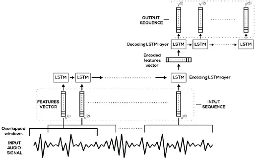
have been shown to outperform state-of-the-art algorithms especially in problems that can be naturally represented via a sequence-to-sequence model, as for example in Handwriting Recognition [14] and Natural Language Processing [15][16]. The basic sequence-to-sequence approach, introduced and now widely popular in Machine Translation [22][23][24], consists in the use of a LSTM cell to encode an input sequence of variable length into a vector of numbers. Hence, a dual LSTM cell can be used to generate the output sequence according to the prediction to be performed, starting from the vector of numbers encoding the input. Due to the generality of this Encoding-Decoding procedure, the extension to several stacked layers is straightforward. For the same reasons, it can be easily adapted to our problem, due to the nature of the audio signal as a continuous stream of data. Indeed, assuming to represent an input frame by a feature vector, the audio signal is represented by a sequence of vectors. Hence, the network is trained to reproduce the sequence itself by minimizing the reconstruction error when processing the sequence of input vectors. This model, performing ND for AS tasks, has been already proposed in [18], showing to outperform classic approaches. A visual representation of the architecture is depicted in figure 1.

The aim of this work is to analyse the relation between the quality of the information extracted at a feature level with the one learned by the RNNs. In particular, we start by extracting a feature representation 𝑥(𝑖)_{of the audio signal, which will be explained in more details in the following of his}

section. This representation is computed on a window 𝑤 composed by a certain number of samples from the raw audio signal, expressing a specific characterization of the input over a given interval. The width 𝑤 of this window is fixed in advance, and so is the amount of information embodied by the generated representation. Hence, a sequence of length 𝑠 of these feature vectors is assembled in order to be fed to the learner, covering a certain time interval 𝐼. The obtained interval 𝐼 is proportional to the window size 𝑤 and to the length of the sequence 𝑠. In particular, if we pose 𝑟 = 1 − ℎ, where ℎ is the rate of overlap between two consecutive feature windows, the input size 𝐼 spans over a temporal interval equal to: 𝐼 = 𝑤 + (𝑠 − 1) ⋅ 𝑟𝑤 = 𝑤 ⋅ [1 + 𝑟(𝑠 − 1)]. A sketch of how the signal is fed into the processing architecture is depicted in figure 1. A first part of the experimental analysis consists in comparing the performances obtained by increasing 𝑠 while keeping 𝑤 fixed. Moreover, we also propose a comparison on different configurations by covering the global input window 𝐼 in different

Figure 1. Global description of the Auto-Encoder architecture composed by Encoding and Decoding LSTM layers to compress and reconstruct the provided feature representation of input

(5)

4 1234567890

ways while maintaining the rate 𝑤/𝑠 constant. A remark has to be done on the case 𝑠 = 1, since in this case the RNNs architecture collapses into a standard Auto-Encoder (AE) [25] with one hidden layer to perform dimensionality reduction, i.e. we have:

ℎ𝑢 < |𝑥| = |𝑦| (1) where ℎ𝑢 is the number of hidden units and |𝑥| = |𝑦| are the dimension of both the input and the (reconstructed) output vectors. The size of the hidden layer is chosen to be smaller than the size of the original input to prevent the network from learning trivial configurations.

3. Experiments

As already said, we focus on the exploration of the correlations of temporal intervals of different size and type. Since many investigations on the best features for ASR task can be found in the literature 0, we avoid further explorations on this part, focusing on the behaviour of the representational agent w.r.t. to a fixed input representation. The features are extracted exploiting the librosa package [26] by computing for each window of 𝑤 samples the Zero-Crossing Rate (ZCR), 20 Mel-frequency cepstral coefficients (MFCCs) and their 20 derivatives (computed by the first order method), since similar configurations are proved 0[6][27] to embody a good general representation in many ASR task, both in speech and non-speech environments. Each extracted feature is then normalized to null mean and standard deviation equal to one. The window size 𝑤 has been varied between 4096 and 32798 samples as reported in table 1, while keeping 𝑟 = 0.25 fixed. In table 1 we reported the real-time window 𝐼 obtained by varying the window size 𝑤 and the length 𝑠 of the sequence processed by the encoding LSTM module. As already said, 𝑠 = 1 indicates that the input feature vector is processed by a static Auto-Encoder. In this case, since the decreasing rate of 𝑠 (0.2 instead of 0.5) is different w.r.t. the ones among the other sequences, the 𝑤 is adapted to obtain a coherent window in term of real world time.

Because of the difficulty in finding publicly available datasets, audio tracks (sampled at 44100 kHz)have been generated by recording a week plus one day of daily activity of the help desk of the library of the Engineering Department at the University of Siena in the time interval 8AM – 8PM. An environmental microphone was placed in a location with a large variety of sounds and interactions, but governed by well-defined social norms so as to generate data as close as possible to a potential critical working environment such as bank branches. The test set was generated by placing artificial anomalies at different random instants of the additional day, so as to have a simple and reliable labelling process. Different classes of anomalies have been recorded providing samples of both human interactions, like crying or screaming, and mechanical sounds (electronic screwdriver, drill, grinder etc). These additional sounds have been later mixed into the original audio samples exploiting the pydub library.

Table 1. Real time interval length (in seconds) corresponding to the input window size analysed in each configuration, composing the feature extraction part and the sequence computed by the agent.

Input Window Size 𝐼 (seconds) Sequence

Length 𝑠 (input steps)

Window Size 𝑤 (samples)

4096 8192 16384 32768 40 3.71 7.43 14.86 29.72 20 1.85 3.71 7.43 14.86 10 0.92 1.85 3.71 7.43 5 0.46 0.92 1.85 3.71 1 0.09 0.18 0.46 0.92

(6)

1234567890

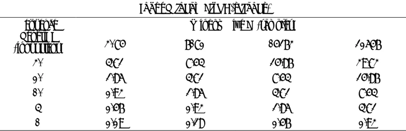
The network is implemented using the Keras framework [28][29]. Both the encoding and decoding LSTMs are composed by 512 units for each gate (with sigmoid activations), whereas the static AE contains 30 units in its hidden layer (with ReLU activation). A validation set (30% of training samples) has been held out to stop the optimization when the reconstruction error, evaluated as the mean squared error (MSE) between the input and the output sequences, stops to decrease. In table 2 we report the Area under the ROC (AUC) obtained in each setting to evaluate the general behaviour of each model. To give an idea of the classification performances, in table 3 we reported the F1-score obtained when selecting the threshold at the point in which the ROC crosses the diagonal.

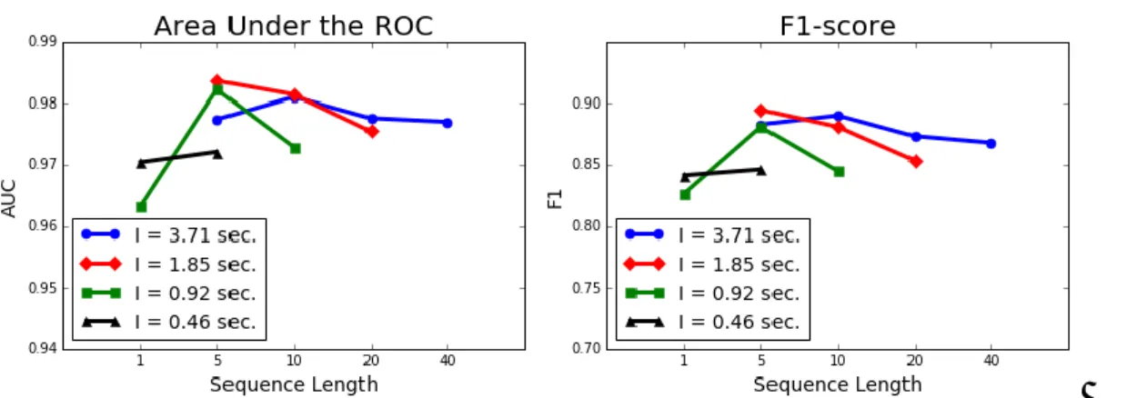
The results are plotted in figure 2, while figure 4 depicts the classification performances varying the size of the features extraction window and the length of the network input sequence while keeping 𝑤/𝑠 constant. In figure 3 we show the behaviour of the reconstruction error from different models in presence of an anomaly. In figure 2 we can observe how in general the RNN performs better than the static AE. Best performances are achieved for each 𝑤 at 𝑠 = 5, except from the shortest window with 𝑤 = 4096. In this case, increasing the length of the processed sequence helps to get close to the results obtained by using wider windows. On the other hand, for larger windows the extension of the input sequence leads in general to a degradation of the performances, especially for the largest one with 𝑤 = 32768. This could be due to the harder training task implied by the longer input sequence, and we leave as a future work to analyse if this issue can be mitigated by increasing the number of units in the LSTM layers. In the right plot of figure 3, it is possible to observe how the processing of long sequence produces a smoother reconstruction error, which implies a reduction of the precision on Table 2. Area Under the ROC Curve (AUC) evaluated on different running varying both the window

size and the length of the sequence processed by the LSTM modules of the ANN. AUC

Sequence Length 𝑠 (input steps)

4096 8192 16384 32768 40 0.9770 0.9716 0.9537 0.9153 20 0.9755 0.9776 0.9724 0.9514 10 0.9729 0.9814 0.9810 0.9706 5 0.9721 0.9822 0.9836 0.9774 1 0.9480 0.9784 0.9704 0.9632

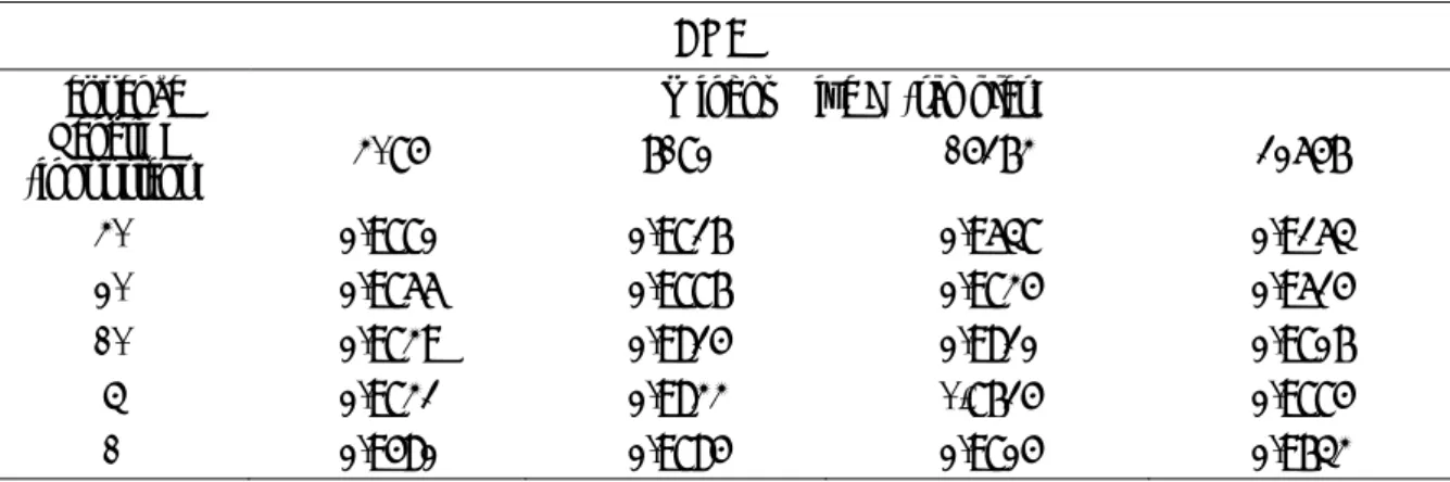
Table 3. F1-score evaluated on different running varying both the window size and the length of the sequence processed by the LSTM modules of the ANN.

F1-score Sequence

Length 𝑠 (input steps)

4096 8192 16384 32768 40 0. 8680 0. 8653 0. 8194 0. 7213 20 0. 8537 0. 8734 0. 8678 0. 8115 10 0. 8449 0. 8810 0. 8902 0. 8648 5 0. 8461 0. 8808 0. 8946 0. 8829 1 0. 7787 0. 8684 0. 8413 0. 8264

(7)

6 1234567890

the anomalies boundaries. Another factor to be considered is the width of the temporal window expressed by the parameter 𝑤. Indeed, the anomalies are collapsed into a smaller number of frames with a large window, raising the detection difficulty. An opposite trend can be observed in the left plot of figure 3. In the case 𝑠 = 1 the reconstruction error shows a higher variability, proving that, as a matter of fact, the static model seems to provide a poorly representation. In figure 4 we reported a comparison among the results obtained by processing configurations with constant rate 𝑤/𝑠 (following the diagonals of table 1). The sequential approach seems to introduce fundamental improvements even in these sense, still confirming the issue of processing long input sequences.

Figure 2. Area Under the ROC (AUC) and F1-score, respectively on the left plot and the right one, obtained varying the sequence length s and the window size w.

Figure 3. Reconstruction error on a slice of input stream in presence of anomalies with both short and long durations, obtained with models trained varying the input sequence length s.

Figure 4. Area Under the ROC (AUC) and F1-score, respectively on the left plot and the right one, obtained varying the sequence length s and the window size w. The comparing is reported by

(8)

1234567890

4. Conclusions

This work studied the application of a sequence-to-sequence model to the problem of identifying abnormal events in an audio input. The proposed solution is purely unsupervised and requires only a stream of normal audio to be trained. This paper also presents an investigation about the importance of considering the temporal sequence when representing an audio signal. The showed results confirm the expected hypothesis that sequential models should work better when dealing with data characterized by an explicit temporal order. Indeed, the static approach, obtained by processing single input frames of a given temporal size, seems to provide a worse representation in each analyzed setting, even when the effectively processed interval of time is the same as the sequential approach. This result seems to be general w.r.t. the used feature representation, since the recurrent modules do not receive any additional information, except from the one produced by correlating consecutive input frames. The study suggests that there is an optimal length in the processed sequences as increasing too much the length of the input sequences leads to a degradation in the classification accuracy. As future work, we plan to investigate alternative architectures limiting the reconstruction of the output sequence, which is very hard to train. For example, once the encoding of the sequence is obtained, the decoder can be used to generate only the last input frames instead of the whole input sequence.

Acknowledgments

We wish to thank Banca Monte dei Paschi di Siena (Siena, Italy) that provided the founding and the main proposals for this research.

References

[1] Sharan R V and Moir J T 2016 Neurocomputing 200 22-34

[2] Orio N et al. 2006 Foundations and Trends in Information Retrieval 1 1-90 [3] Cowling M and Sitte R 2003 Pattern Recognition Letters 24 2895-907

[4] Chachada S and Kuo J 2013 Signal and Information Processing Association Annual Summit and Conference (APSIPA) 1-9.

[5] Crocco M, Cristani M, Trucco A, and Murino V 2016 Computing Surveys (CSUR) 48 52

[6] Choi W et al. 2012 Advanced Video and Signal-Based Surveillance (AVSS) 118-123

[7] McLoughlin I et al. 2015 IEEE/ACM Transactions on Audio, Speech, and Language Processing 23 540-52

[8] Pimentel M, Clifton D, Clifton L and Tarassenko L 2014 Signal Processing 99 215-49 [9] Williams G et al. 2002 International Conference on Data Mining 709-12

[10] Bishop C M 1994 IEE Proceedings-Vision, Image and Signal processing 141(4) 217-22 [11] Tarassenko L et al. 1995 4th International Conference on Artificial Neural Netowrks 442-7 [12] Foggia P et al. 2016 IEEE Transaction on Intelligent Transportation Systems 17(1) 279-88 [13] Ntalampiras S, Potamitis I and Fakotakis N 2011 IEEE Transaction on Multimedia 13 713-9 [14] Graves A et al. 2009 IEEE Transaction on pattern analysis and machine intelligence 855-68 [15] Sundermeyer M et al. 2012 13th Annual Conference of the International Speech

Communication Association

[16] Sutskever I et al. 2014 Advances in neural information processing systems 3104-12  [17] Hochreiter S and Schmidhuber J 1997 Neural Computaion 9 1735-80

[18] Marchi E et al. 2017 Computational intelligence and neuroscience [19] Werbos P 1990 Proceedings of the IEEE 78(10) 1550-60

[20] Hochreiter S et al. 2001 A field guide to dynamical recurrent neural netoworks. IEEE Press [21] Bengio Y 1994 IEEE transaction on neural networks 5(2) 157-66

[22] Kalchbrenner N and Blunsom P 2013 EMNLP 3(39) 413 [23] Graves A 2013 arXiv preprint (arXiv:1308.0850)

(9)

8 1234567890

[25] Ranzato M et al. 2006 Advances in Neural Information Processing Systems 19 1137-44 [26] McFee B et al. 2015 Proceedings of the 14th python in science conference 18-25

[27] Antti et al. 2006 IEEE Transaction on Audio, Speech and Language Processing 14 321-9 [28] Chollet F et al. 2015 https://github.com/fchollet/keras

Auto-Associative Recurrent Neural Networks and Long Term Dependencies in Novelty Detection for Audio Surveillance Applications

IOP Conference Series: Materials Science and Engineering

Auto-Associative Recurrent Neural Networks and

Long Term Dependencies in Novelty Detection for

Audio Surveillance Applications

Related content

Auto-Associative Recurrent Neural Networks and Long

Term Dependencies in Novelty Detection for Audio

Surveillance

Applications