DOTTORATO DI RICERCA IN
Ingegneria Biomedica, Elettrica e dei Sistemi
Ciclo 31°
Settore Concorsuale:
ING-INF/04 - Automatica
Settore Scientifico Disciplinare: 09/G1 - AutomaticaPERCEPTION AND LOCALIZATION TECHNIQUES FOR NAVIGATION IN
AGRICULTURAL ENVIRONMENT AND EXPERIMENTAL RESULTS
Presentata da:
Flavio Callegati
Coordinatore Dottorato
Supervisore
In the last decades automation has had an extraordinary expansion, whose ex-amples are found not only in industry, but anywhere around us in everyday life: cars, automatic machines, robots and drones, both for modeling and supporting humans. The concept of automation, as the name implies, consists in automating certain actions, devices or mechanisms, with the aim of making them faster and less tiring, in perspective less expensive or dangerous for humans. Thanks to the development of new technologies, in mechanics and electronics, which allow to get smarter and more compact solutions, and more powerful computers, automation is constantly expanding in new fields and wherever its application can provide ad-vantages for humans.
In recent years research has led to an expansion of automation, among others, in the agricultural field. Notoriously, it is a very hard work environment, where the operator manually carry out any job, often in extreme weather conditions or anyway heat, cold and rain, or simply where the working hours last from dawn to sunset. Due to the high investment of time and energy, considerable benefits can be gained in this field by automating certain operations, replacing or simply supporting the human operator. Following these motivations, appeared the first, more or less experimental robots, able to automatically plow a field, by perform-ing a grid by means of GPS receiver, or to sow, usperform-ing cameras and artificial vision algorithms.
Recently, research in this field is turning towards the development of increasingly autonomous robots, able to take care of di↵erent tasks and avoid obstacles, and so flexible to collaborate and interact with human operators. Indeed, expand-ing perception and computational capacity of these drones, smart robots can be created, capable of locating themselves, accepting whole missions from the
opera-tor, autonomously evaluating the conditions for carrying them out, and collecting data from the surrounding environment. The latter can then be shared with the operator, informing him about the soil moisture rather than the critical health con-ditions of a single plant. Thus borns the concept of precision agriculture, in which the robot performs its tasks according to the environment conditions it detects, distributing fertilizers or water only where necessary, thus optimizing treatments and its energy resources.
The proposed thesis project, which consists in the development of a tractor pro-totype able to automatically act in agricultural semi-structured environment, like orchards organized in rows, and navigating autonomously by means of a laser scan-ner. In particular, the thesis is divided into three steps. The first consists in design and construction of a tracked rover prototype, which has been completely realized in the laboratory, from mechanical, electric and electronic subsystems up to the software structure. The second is the development of a navigation and control system, which makes a generic robot able to move autonomously within rows, and from one row to the next, using a laser scanner as main sensor. To achieve this goal, an algorithm for rows estimation has been developed, letting the robot to locates itself within the environment. Moreover, a control law has been designed, which regulates the kinematics of the rover and computes desired velocities. Once the navigation algorithm has been defined, it is necessary to validate it. Indeed, third point consists of experimental tests, with the aim of testing both robot and developed autonomous navigation algorithm, whose results are presented in the last part of the thesis.
Le prime persone che vorrei ringraziare sono i miei genitori, Loris e Teresa, per avermi trasmesso la fiducia in me stesso che mi ha permesso di raggiungere tanti obiettivi e per averla rinforzata nei momenti difficili. Ringrazio di cuore la mia ragazza Chiara, per essermi stata vicino e avermi sempre sostenuto, sia durante gli studi che nel corso del dottorato. Un grazie particolare va a Nicola, per i consigli e l’esperienza che mi ha trasmesso, ma anche per le belle ore passate insieme, in lab-oratorio e durante i viaggi. Ringrazio anche i ragazzi del Team Rover, Alessandro e Roberto, sia per le risate che per la collaborazione nel raggiungimento di ogni risultato. Un grazie va anche al mio coordinatore, Lorenzo, per la sua guida e per i preziosi consigli che mi ha dato in questi anni. Ultimo ma non ultimo, ringrazio Rob, che mi ha guidato durante la tesi magistrale e ispirato ad iniziare il percorso verso il dottorato.
Abstract i 1 Automation in Agriculture: State of the art 11
1.1 Introduction . . . 11
1.2 Motivations . . . 11
1.2.1 Navigation for tasks implementation . . . 12
1.2.2 Peculiarities of the Agricultural Environment . . . 12
1.2.3 Absolute and relative localization . . . 13
1.3 State of the art . . . 16
1.3.1 Navigation in agricultural environment . . . 16
1.3.2 Smart agricultural robotic platforms . . . 20
1.3.3 Navigation in structured agricultural environment . . . 23
1.4 Conclusions . . . 29
2 Platform description 31 2.1 Introduction . . . 31
2.2 Mechanical description . . . 32
2.2.1 Frame and mechanical structure . . . 32
2.2.2 Tracks . . . 33 2.2.3 Tool Modules . . . 34 2.3 Electrical description . . . 35 2.3.1 Lithium Batteries . . . 36 2.3.2 Drivers . . . 37 2.3.3 Motors . . . 38 2.3.4 Brakes . . . 38
2.3.5 DC-DC Converters . . . 38
2.3.6 Lead Battery . . . 39
2.3.7 Winch Circuit . . . 39
2.4 Electronic Box and Sensors . . . 39
2.4.1 Electronic Box . . . 39
2.4.2 Buttons Panel . . . 46
2.4.3 Sensors . . . 48
2.4.4 External Devices . . . 50
2.5 Conclusions . . . 52
3 Developed Navigation Tecniques 53 3.1 Introduction . . . 53
3.2 Reference Frames . . . 53
3.3 Navigation . . . 55
3.4 Structured Environment and Internal Model . . . 57
3.5 Hough Transform Upgraded . . . 58
3.6 N-Hough Transform Upgraded . . . 62
3.7 Robot Control Law . . . 65
3.8 Robot Control within rows . . . 67
3.9 Conclusions . . . 68
4 Software structure 71 4.1 Introduction . . . 71
4.2 Onboard Controller . . . 72
4.3 HMI-Robot Control Interaction . . . 74
4.4 Human Machine Interface . . . 75
4.4.1 Screens Description . . . 76
4.5 Robot Control . . . 86
4.5.1 ROS Messages . . . 87
4.5.2 ROS Nodes . . . 91
4.5.3 User-defined Mavros Plugins . . . 105
4.5.4 ROS Packages . . . 107
4.5.5 Robot Control launch . . . 112
5 Experimental tests 115
5.1 Introduction . . . 115
5.2 Goals . . . 116
5.3 Experimental setup . . . 117
5.4 Experimental results . . . 119
5.4.1 Electric and mechanical features . . . 119
5.4.2 Autonomous navigation features . . . 134
5.5 Conclusions . . . 141
6 Conclusions and Future Developments 143 6.1 Conclusions and Final Discussions . . . 143
6.2 Next Developments and Future of the Project . . . 145
A Sensors 151 A.1 Encoders . . . 151
A.2 GPS . . . 153
A.3 IMU . . . 155
A.4 Ultrasonic sensors . . . 156
A.5 Laser Scanner and LIDAR . . . 157
A.6 Cameras . . . 159
A.7 Infrared cameras . . . 160
B Estimation algorithms 161 B.1 Introduction . . . 161
B.2 RANSAC . . . 163
B.3 Hough Transform . . . 166
C Software data structures 171 C.1 Field parameters . . . 171
C.2 Robot class . . . 172
1.1 Ruts due to tractor passage on muddy terrain . . . 13
1.2 Wheat field, open field environment example . . . 14
1.3 Vineyard (left) and crop field (right) organized in row structures . . 15
1.4 Robotic melon harvester pulled by tractor . . . 17
1.5 Dual GNSS-RTK receiver mounted on the tractor roof . . . 19
1.6 Agrobot operating in the field . . . 21
1.7 Experimental robot farmer . . . 22
1.8 HMI Mission assignment (left) and monitoring (right) screens . . . 22
1.9 Raw (left) grey-scale image and developed elevation map (grey) of the rows . . . 24
1.10 Picture of soybean field . . . 25
1.11 Experimental platforms: tractor-pulled cultivator (left) and au-tonomous robot (right) . . . 26
1.12 Experimental platform, equipped with a couple of 2D laser scanners 26 1.13 Experimental car moving within rows (left) and LIDAR environ-ment perception (right) . . . 27
1.14 Row change proposed trajectories: lamp (left), clothoid(center) and thumb(right) . . . 27
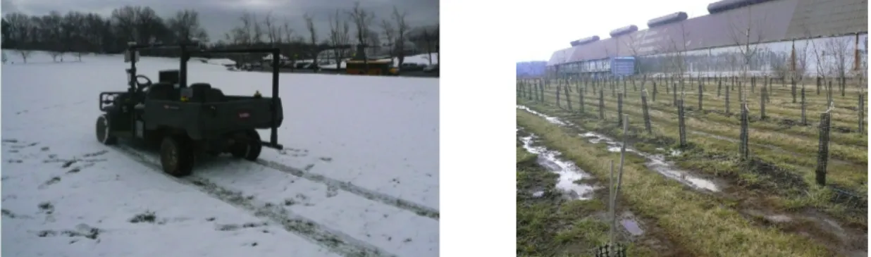
1.15 Eperimental tests environments, with presence of snow (left) and mud (right) . . . 28
2.1 Picture of the developed agricultural robot. . . 32
2.2 Picture of the robot construction, showing the aluminium frame. . . 33
2.4 Mechanical system for plugging and managing tools (left) and detail
of the quadrilater structure (left). . . 34
2.5 Detail of lithium and lead batteries installed on the robot. . . 36
2.6 Aluminium plate on which drivers, converters and contactors are installed. . . 37
2.7 View of the whole content of the electronic box. . . 40
2.8 Intel NUC model D54250WYKH, external and inner view. . . 41
2.9 Arduino Pro Mini microcontroller. . . 43
2.10 Arduino relay module. . . 43
2.11 Cooling system of the electronic box, composed by cooling fans (left side) and temperature sensor (right side) . . . 44
2.12 Arduino Mega 2650. . . 45
2.13 IXXAT USB-CAN Interface. . . 46
2.14 Detail of the electric box external buttons and switches. . . 47
2.15 Detail of laser scanner and gps installed on the sensors bar. . . 48
2.16 10 degrees of freedom IMU . . . 49
2.17 Ublox GPS receiver . . . 49
2.18 Velodyne LIDAR VLP-16 (left) and sensor data collected within rows of a plum field (right) . . . 50
2.19 Trimble R8s GNSS System. . . 51
2.20 Logitech joypad . . . 52
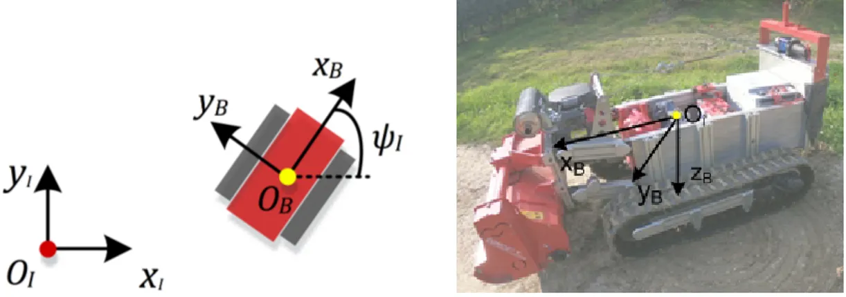
3.1 Representation of the adopted pseudo-inertial NED frame . . . 54
3.2 Body frame representations, respect to the inertial frame (left) and to the real robot structure (right) . . . 54
3.3 Representation of the laser frame, respect to the body frame . . . . 55
3.4 Example of view within rows . . . 58
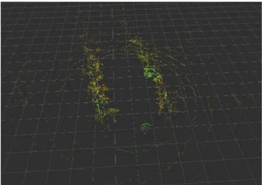
3.5 LIDAR data collected within two rows in a plum field . . . 59
3.6 Distances and angles returned by the Hough transform algorithm . 60 3.7 Research grid of the Hough transform algorithm . . . 60
3.8 Research grid of the proposed localization algorithm within rows . . 62
3.9 View of orchard rows from the outside of the structure . . . 62
3.10 LIDAR data collected outside the rows of a plum field . . . 63
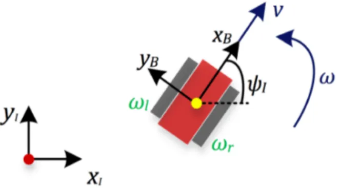
3.12 Research grid of the proposed localization algorithm outside the rows 65 3.13 Representation of inertial and boby frames, and kinematics control
inputs . . . 66
3.14 Conceptual scheme of the adopted lateral distance control loop . . . 68
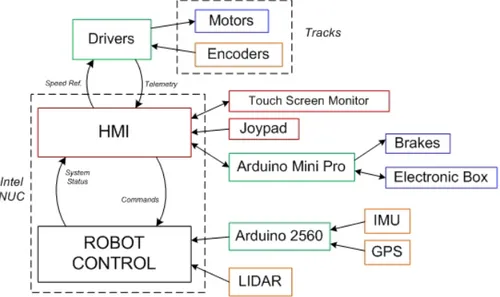
4.1 Block scheme of sotfware architecture and most important inner and outer connections . . . 72
4.2 HMI initial screen . . . 76
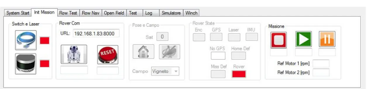
4.3 HMI panel for starting the communication with the robot and set-ting the foundamental parameters . . . 79
4.4 HMI panel for test definition, assignment and monitoring . . . 81
4.5 HMI panel for setting missions, send them to he robot and monitor their progesses . . . 82
4.6 HMI panel for setting and starting experiments for testing the robot tracks movements . . . 83
4.7 HMI panel for setting log files detail . . . 85
4.8 HMI panel for the robot simulator . . . 85
4.9 HMI panel for winch remote control . . . 86
4.10 Representation of the row state machine, with possible states and most important admitted transitions . . . 92
4.11 Functional scheme of the most important ROS nodes implementing the Robot Control . . . 113
5.1 Robot equipped with mower (left) and then with LIDAR and low cost GPS (right) . . . 117
5.2 Reference speed tracking during straight trajectory at constant speed120 5.3 Mechanical power asked by the tracks during straight trajectory at constant speed . . . 121
5.4 Mechanical and electric powers asked by the robot during straight trajectory at constant speed . . . 122
5.5 Reference speed tracking during straight trajectory at di↵erent speed values . . . 123 5.6 Motor torques during straight trajectory at di↵erent speed values . 123 5.7 Battery voltage during straight trajectory at di↵erent speed values . 124
5.8 Drivers temperatures during straight trajectory at di↵erent speed
values . . . 125
5.9 Instance of the steering test . . . 126
5.10 Reference speed tracking during steering maneuver . . . 126
5.11 Motor torques during steering maneuver . . . 127
5.12 Electric powers asked by the robot during steering maneuver . . . . 128
5.13 Images from the experimental test, with the rover moving at low (left) and high speed (right) . . . 129
5.14 Reference speed tracking during stress test . . . 129
5.15 Motor torques during during stress test . . . 130
5.16 Mechanical powers asked by the robot during stress test . . . 131
5.17 Drivers temperatures during stress test . . . 131
5.18 Absorbed currents during stress test . . . 132
5.19 Battery voltage during stress test . . . 133
5.20 Image from the autonomous navigation experiment (left), with the manual controller placed on the robot electronic box, and screen from the onboard computer, showing the lateral estimated lines (right). . . 134
5.21 Lateral distances between robot and estimated row lines during au-tonomous navigation . . . 135
5.22 Lateral distance error between robot and estimated row lines during autonomous navigation . . . 136
5.23 Relative orientation between robot and estimated row lines during autonomous navigation . . . 137
5.24 Motor reference velocities during autonomous navigation . . . 138
5.25 Image from a localization experiment, taken during a row change. . 139
5.26 Online row lines estimation while the robot is curving in left direc-tion, during a row change. . . 139
5.27 Online row lines estimation while the robot is curving in right di-rection, during a row change. . . 140
A.1 Absolute encoders schemes, with binary 4 bits (left), Grey 4 bits (center) and 7 bits (right) codings . . . 152
A.2 Incremental encoder scheme, representing channels A and B and
the zeroing reference mark . . . 152
A.3 3DR (left) and uBlox (right) GPS receivers . . . 153
A.4 Trimble R8s GNSS-RTK receiver . . . 155
A.5 Ten (left) and six (right) degrees of freedom IMUs . . . 156
A.6 Example of low-cost ultrasonic sensor . . . 156
A.7 Example of ground (left) and aerial (right) laser scanner data . . . 157
A.8 Hokuyo UTM-30LX-EW planar laser scanner (left) and example of a gimbal model (right) . . . 158
A.9 Examples of 3D Velodyne LIDARs: HDL-64E (left), HDL-32E (cen-ter) and VLP-16 (right) . . . 158
A.10 An XBOX 360 Kinect, example of common stereo-camera . . . 159
B.1 Realistic LIDAR pointclouds, collected within (left) and outside (right) orchard rows . . . 162
B.2 Discrimination of inliers (blue dots) and outliers (red dots) on real pointcloud data . . . 162
B.3 Least Squares line extraction, a↵ected by the presence of outliers . . 163
B.4 RANSAC algorithm iteration, where the points close to the sample are counted . . . 165
B.5 Pointcloud items considered by the Hough transform algorithm . . . 167
B.6 Beams of lines generated by the Hough transform algorithm . . . . 168
B.7 Representation of a possible resulting vote matrix. . . 168
C.1 Representations of the field row structure informations . . . 172
Automation in Agriculture: State
of the art
In this chapter concepts of automation and robotics application in agriculture are described in details, both highlighting environment features and related difficulties, and describing last decades progresses, applications and state of the art.
1.1
Introduction
Proposed research work was developed in the context of precision agriculture and concerns, in particular, navigation in agricultural semi-structured environ-ments. Before proceeding with the proposed approaches and the obtained results, it is better to clarify the context and the state of the art concerning this research field. In this chapter a brief report about state of art will be presented, focusing on navigation, control and localization techniques, showing and discussing di↵erent examples and gradually motivating methods and techniques applied in this work.
1.2
Motivations
In this section some aspects of the environment and application of this research project will be discussed, in order to better contextualize it, clarify the difficulties and finally motivate approaches and choices.
1.2.1
Navigation for tasks implementation
What is expected by an agricultural robotic system is the ability to carry out di↵erent types of tasks in the field, supporting or replacing human operators. This concept holds for any platform, from the simplest one dedicated to a single task (see first example in section 1.3) to more intelligent and modular robotic systems, equipped with advanced user interfaces (see subsection 1.3.2). The main characteristics of such a robotic platform must be the dimensions, the traction capacity, the autonomy and the ability to host onboard or tow di↵erent modules or tools. This means that the basic component of an agricultural robotic platform is a tractor, or rover, wheeled or tracked, with di↵erent features depending on the application. Moreover, any task of the rover can be conceptually splitted into two di↵erent actions, to be carried out simultaneously and for the entire mission duration:
- Autonomous navigation in the orchard
- Management of the onboard tools for task implementation
The latter is related to the specific mission and can range from activation of a camera, for inspections, to ignition of a an air-blast sprayer for treatments distri-bution or managament of a mower. Navigation, or autonomous movement ability, on the other hand, is a common aspect of any mission, from less to most complex ones, and a fundamental requirement for any practical application of automation in the agricultural field.
1.2.2
Peculiarities of the Agricultural Environment
Agriculture environment is characterized by some specific features that make the development of navigation solutions very challenging. Harvesting, pruning, falling branches, missing trees or simply variations due to seasonal changes, cause not uniform conditions in terms of recurrent features. In addition, there is a high variation of the light conditions within rows, related to di↵erent coverage of trees and kind of canopy. Moreover, the environment is often a↵ected by the presence of wind, making it (in terms of features) extremely variable. Consequently, the po-sition estimation tends to be inaccurate. Finally, since the object of these project
is a land vehicle, characteristics of the terrain become part of the problem. Es-pecially during the cold season, this can be rough and a↵ected by the presence of snow, rather than puddles or mud, with two main consequences:
• After many passages on wet ground deep pools or holes tend to form, where the vehicle risks to get bogged down or stuck (see figure 1.1).
• Vehicle slippage on soft surfaces prejudice the encoders measurements, which tend not to reflect the actual kinematics of the vehicle. In order get a precise localization, it is necessary to correct encoders data or merge with other sensors not a↵ected by ground slippage.
Figure 1.1: Ruts due to tractor passage on muddy terrain
Last but not least, occlusions in GPS are recurrent due to dense vegetation, while ionosphere conditions may cause errors, in absence of di↵erential corrections. All the previous facts make the problem of localization and mapping extremely chal-lenging and, in turn, the development of robust navigation strategies hard to be addressed.
1.2.3
Absolute and relative localization
GPS receivers (see section A.2) have always been a fundamental component of many outdoor navigation approaches (see section 1.3.1). Indeed, absolute position on the earth’s surface can be known in any meteorological condition, but provided that satellite coverage is sufficient. However, there are a lot of drawbacks in using GPS technology:
• GPS position is not very precise: for this reason GNSS-RTK receivers (see section A.2) or sensor fusion techniques are employed to achieve better ac-curacy.
• This kind of solutions are efficient as long as the robot is in open field envi-ronments (see figure 1.2), i.e. until there are no constructions, rather than thick vegetation or terrain conformations that cause a decrease or complete lack of satellite coverage.
• GPS, and sensors commonly used for data fusion, do not provide any kind of perception about the surrounding environment. Indeed, the GPS provides an absolute position, encoders (subsection A.1) the motors rotation speeds, and IMU gives back attitude, rotations or accelerations.
Figure 1.2: Wheat field, open field environment example
For these reasons, GPS-based navigation requires a perfect knowledge of the sur-rounding environment, in order to be feasible. This condition, in an outdoor or agricultural environment, is difficult to achieve, as unexpected obstacles can always be present and it is necessary to take into account seasonal changes in vegetation, branch growth or fallen branches due to strong wind, rather than puddles or muddy or icy areas, due to adverse weather conditions. Therefore, it is necessary to use proximity sensors, such as ultrasonic sensors (section A.4) or LIDAR (section A.5), which allow to evaluate the conformation of the ground or surrounding vegetation and to detect the presence of any obstacle on the path.
Moreover, the necessity of the GPS signal for navigation tends to reduce when working in a structured or semi-structured environment, like crops organized in
Figure 1.3: Vineyard (left) and crop field (right) organized in row structures
rows (see 1.3). Within this environment, the absolute position is not so important for navigation as the relative one respect to the surrounding structure. Indeed, known the lateral distance, the robot can move keeping the row center , while from the front view it is able to assess any obstacle presence. Using LIDAR or cam-eras (section A.6), and real-time processing architectures, the robot will be able to locate itself within rows, create a map and evaluate its attitude with respect to the lines of trees. In this context, GPS covers a marginal role, being used to have redundant information about rover position in a row or in another one, or know its proximity to the extremities of the rows themselves.
In order to conclude this discussion about localization and sensors and motivate the next projectual choises, a comparison between the two most advanced proximity sensors currently used in agriculture, i.e. cameras and LIDAR, is proposed. The most important advantages and drawbacks of the two devices can be summarized as follows:
• Cameras are lighter and less expensive than laser scanners and can realize all the typical functions of LIDARs, from mapping to localization, supported by colors that characterize objects and surrounding environment.
• On the other hand, the application on a tractor does not involve problems related to sensor size or weight. In addition, LIDAR has a greater range. Moreover, what is foundamental for navigation is the distance with respect to surrounding environment, rather than details or colors of the di↵erent objects, which are contained in camera images.
• Working outdoor, the robot should navigate in various weather conditions like rain, wind, darkness or fog, while the sensor could get dirty due to wind
or dust generated during work. For this point of view, LIDARs seems to behave better than cameras, since they are tested for outdoor environments and their performances are not a↵ected by light conditions.
In view of these motivations, LIDARs and cameras seem to be both suitable for providing environment perception and supporting outdoor autonomous naviga-tion. However, in the proposed agricultural application a 3D laser scanner has been chosen, expecially for its capacity of working in adverse weather conditions, but with the knowledge of its high cost and drawbacks.
Next experiments will show if this choice is actually correct, or further evaluations are needed. For example, it could emerge that the proposed navigation algorithms do not need so high sensor performances, and maybe just a less expensive 2D laser scanner will be employed. Of course, also a stereo camera could be a suitable choice, expecially if some fruit or plant deseases detection algorithms will be im-plemented onboard, in which evironment color details are foundamental, and the whole surroundings perception can be provided by means of a singe sensor.
1.3
State of the art
1.3.1
Navigation in agricultural environment
In the last decades automation and robotics applications are constantly ex-panding in many fields, leading to considerable savings in terms of cost, as well as fatigue or time for the human operator. Agriculture has followed this trend and has been subject of many research projects, which seek new solutions to automate operations like inspection, planting, plowing or harvesting. These approaches vary widely, ranging, for example, from the simplest ones based on single sensors, as in the case of GPS-based solutions used for automating plowing or threshing over large areas, to the one using entire sensor suites, whose data are merged to obtain more and more precise and reliable localization in the environment. Depending on the applications, inexpensive solutions can be provided, taking advantage of cheap sensors, up to more expensive and performant ones, using for example modern LIDAR sensors, through which visual odometry, mapping and obstacle detection can be implemented, or GNSS-RTK receivers, capable of providing centimetre
ac-curacy.
One of the first applications is an automatic control system for melon harvesting [25], developed about twenty years ago by an Israeli research group. The experi-mental platform was composed by a cartesian robot manipulator, having the task of picking fruits, mounted on a mobile platform pulled by a tractor along the rows (see figure 1.4). In this application, the fundamental component for melon detec-tion was a camera, whose images were then filtered and enhanced using computer vision algorithms. The result of the experimental tests was a success rate of 85% in melons detection and picking. In this work the robotic harvester control is inde-pendent from the movement along the rows, provided by the tractor, meaning that problems like navigation or localization in the field are not taken into account. The work is indeed focused on fruit detection and cartesian harvester motion control . Di↵erently, in order to automate operations like plowing or fertilizer distribution,
Figure 1.4: Robotic melon harvester pulled by tractor
the movement of the platform has also to be managed and the control problem becomes more complicated. In fact, the system must be able to autonomously es-timate its position in the environment, as well as evaluating slope and consistency of the terrain and detect and manage any obstacles presence. The problems are therefore both at the level of environment perception and trajectory tracking, and of safety, for people, surrounding environment or the robot itself, due to its size and traction capacity.
An example of research about ground prediction for safety reasons is given in [24].This work deals with the problem of navigating in vegetation or farm condi-tions, where terrain characteristics change and vegetation itself can hide holes or obstacles. Here, an online adaptive approach to automatically predict ground
con-dition is presented. Pose estimation is carried out by means of a GPS unit, a 3-axis gyroscope, a doppler radar and encoders on wheels and steering unit. Di↵erently, the ground prediction is based on a couple of stereo cameras and two LADAR sensors. The presented algorithm is not model-based, but relies on a learning ap-proach: the predictions are developed looking forward, with the sensors, and using the vehicle past experience.
In 2000 John Deere company released the Autotrac System, a commercial GPS guidance system available for di↵erent models of its tractors and agricultural ma-chines. Such a system helps the human operator in the steering action, expecially in low visibility conditions, defining a more efficient trajectory and lowering pro-duction costs.
In 2005 a guidance system based only on GPS technology was developed and tested on an autonomous mobile platform [12]. The robot receives waypoints from the user through an RF communication system, by which the UGV position can be monitored on a remote PC. This generic results can be applied in various fields, such as transports, agriculture, and so on. The most important limitation of the approach is the missing of informations aboutrelative position between robot and surrounding environment. Indeed, the vehicle can move anywhere on the earth’s surface, but it is blind to obstacles, terrain conditions, holes and vegetation. Moreover, such a system is efficient only in open or wide spaces, since the preci-sion of a common GPS receiver is about one meter. This limits the possibility to act in narrow environments or performing strict maneuvers, needed to move in a street or in a row of trees. The solutions to that problem could be the adoption of more performant sensors, such as a di↵erential GNSS-RTK receiver. That kind of device can ensure an accuracy of centimeters, but, as a main drawback, has a very high cost. Other approaches could be the installation of distance sensors, by which the system can percept the surrounding environment, or using sensor fusion and combining for example GPS and IMU. The approach proposed in [21] consists in fusing data from a common GPS receiver and proximity sensors. Actually, the lat-ter are not mounted onboard, like lasers or sonars, but landmarks installed in the field and broadcasting their position. When the vehicle approaches those sensors, its position is corrected or calibrated. The main advantage of this system is that the position correction is exact, since the landmark location is perfectly known.
The drawbacks are the position estimation drift, which tends to appear in the path between sensors, and the necessity to prepare or adapt the work environment to the vehicle, precluding its application fields and its flexibility.
In a di↵erent way [15], GPS performances can be improved using multiple, i.e. two or three, GPS receivers placed over the vehicle at a certain mutual distance (see figure 1.5). Through data fusion, for example by means of a Kalman filter,
Figure 1.5: Dual GNSS-RTK receiver mounted on the tractor roof
the position error can be reduced and also the yaw angle (see section 3.2) can be estimated. Since the distance between receivers is obviously limited by the vehicle dimensions, the use of low-cost GPS receivers, with one meter precision, does not produce appreciable results and leads to the necessity of expensive GNSS-RTK sensors. So, even if this approach gives good results in terms of absolute position, has the side e↵ect of being really expensive.
In 2011 a Japanese research group presented an autonomous tractor able to har-vest and move in a rice field [26]. The problem was basically to control the vehicle through a row of plants, then turn to the next one and so on, moving along a sort of grid. The proposed guidance law is based on GPS receiver and IMU, giving respectively global position and heading of the robot.
Another example of GPS-based navigation in agricultural environment is given in [22]. Here a GPS based guidance law is presented, which allows a robot to au-tonomously navigate in a farm environment. The vehicle heading is provided by a digital compass, which provides the capability of steering following a predefined path.
successfully in a narrow environment, such as orchard rows. In [11] an example of this approach is described. Known the exact GPS location of the field and the single rows, a predefined trajectory for the robot can be computed. Then,using a RTK GPS receiver and an IMU, which gives the heading, the system calculates and controls the position error, providing the capability to navigate within the rows of a generic field following the desired path. This kind of approach is nomi-nally correct, but based on a perfect knowledge of the field and on the hypothesis of obstacles absence and no variations in vegetation or ground conformation. The position estimation can be improved fusing data from GPS and a camera. In [20] a small automatic robot is developed, with the purpose of sowing seeds. The vision system builds a local map, identifying the path to follow, and these data si correlated to the GPS coordinates, in order to localize the robot. Thanks to an ultrasonic sensor placed in the front of the vehicle, is also implemented a simple obstacle avoidance task, which stops the robot if some object is detected on its path.
Some examples of robotics and automation applications in the agricultural field have been discussed so far, which are generally based on the specific application, such as rice or melons harvesting, sowing, or polarized towards a navigation idea based on GPS technology. Fasting forward a few years, more recent developments and improvements in this approaches can be observed. This evolution will be dis-cussed in the two following subsections (1.3.2 and 1.3.3), which describes a more conceptual aspect, related to human machine interaction, and an improvement related to environment perception and new generation sensors, respectively.
1.3.2
Smart agricultural robotic platforms
Up to now di↵erent solutions of agricultural robots were presented, basically designed just to navigate in outdoor environment and performing well delimited tasks. The main purpose was to move in the orchard, with a poor or absent interac-tion between robot and human operator, and no particular smart funcinterac-tions. Over time the idea of agricultural robots has evolved and now tends to mean a robotic platform, equipped with a suite of sensors by which it can navigate autonomously in di↵erent kinds of crops, collect data from the field, monitor the health of plants and interact with the user. The described robotic system is generally composed
by a team of robots, i.e. UGVs for the heavy tasks and UAVs for monitor and inspection functions, a user interface, throw which the operator can both moni-tor farm state and assign missions to the system and finally a dynamic database, containing data collected during works and inspections and shared with the user. The last component is a wireless network which covers all the farm and provide communications between robots, database and human operator. So, in this vision of automated farm, the rover, or automatic tractor, becomes just a part of the whole robotic system.
One of the first examples (2015) of this concept is given in [10]. In this work is described ”Agrobot” architecture (see figure 1.6), a smart agricultural robot able to execute many tasks and monitor field conditions, from disease diagnosis to soil analysis and so on. Moreover, part of the project is also the implementation of a cloud service, containing and sharing weather informations, data collected by the robot or treatments parameters. In addition to the basic mechanical and electronic components, the rover is equipped with a wireless communication board, camera and live video transmitter, in order to provide interaction and communication with user or other devices. Moreover, thanks to the presence of distance sensors, cam-era, IMU and GPS receiver, Agrobot can ensure the navigation capabilities needed to autonomously perform tasks and missions in the field.
During the same year, Bergerman and his team presents an agricultural robotic
Figure 1.6: Agrobot operating in the field
system able to navigate autonomously whithin rown of trees and equipped with a remote user interface [17]. The platform is a car-like robot (see figure 1.7), equipped with a 2D LIDAR sensor as foundamental component of the environ-ment perception system. Indeed, navigation is essentially based on encoders and
Figure 1.7: Experimental robot farmer
laser scanners, with no use of GPS. From human machine interfacement point of view, the most interesting progress is the development of a remote interface, run-ning on tablet or laptop, and communicating with the robot onboard computer by means of a wireless network. Through a first screen (see figure 1.8) the user can assign missions to the robot, deciding the field where to work and specifying the rows to go through rather that to skip and defining the desired lateral distance from the trees.
In a second screen (see figure 1.8) the operator can start the mission and monitor its advancements on the di↵erent rows, i.e. see if the work in the single row is completed, has already to start or is in progress.
These interesting examples show the possibility to realize agricultural robotis
forms able to navigate in the farm environment, while autonomously performing di↵erent operations, and even more to interact and communicate with the human operator. This conceptually opens the doors towards a future in which agricul-ture will be completely automated and the farmers have a team of robots, can easily assign missions and monitor their progresses from a remote position. The advanced user interface and the sensor suite whereby robots will be equipped will allow the operator to monitor plants health, detect malfunctions of faults, rather than directly observe the robot at work, thanks to onboard cameras and possibility to streaming data. In this vision all the work is demanded to the robots and the operator can remotely monitor his farm and robot team as if he were present in the field.
1.3.3
Navigation in structured agricultural environment
Up to now (see subsection 1.3.1) some esamples of navigation tecniques in agri-culture field have been discussed, were proximity sensors assumed a marginal role, thus giving little importance to the surrounding environment perception. When operating in a structured or semi-structured environment, such as an orchard or-ganized in rows, knowledge of the absolute position takes on a less significant role in navigation, while the concept of environment perception and relative position respect to the structure becomes more important. Indeed, once a row has been taken, the goal of the robot is just to navigate within the lines of trees and then move to the next rows. This means that the robot only needs to know its relative position within rows, which can be obtained through advanced proximity sensors, combined with computer vision algorithms. Over time, technological progress has made available high-performance sensors, which allow a visual perception of the environment that tends to get closer to the human one: cameras and LIDAR. These sensors returns images or pointclouds (see section A.5) of the surrounding environment. Through computer vision algorithms, sensor data can be enriched, extracting models or features. In agriculture this allows to estimate trees posi-tion or row lines, detect rows entry or exit and navigate inside it, and recognize di↵erent types of obstacles. Exploiting that relative position feedback, a control loop can be designed, in order to keep the tractor in the middle of the corridor environment and, known the rows position, discriminate obstacles not belonging
to the structure. On this basis an obstacle avoidance system can be implemented, with recognition of the obstacle type and precise recovery actions.
Assuming a marginal role, GPS does not necessarily have to guarantee high per-formances. In fact, a common GPS receiver can be employed, whose precision is sufficient to discriminate the row where the robot is moving or to get an idea of proximity to the row extremities. Moreover, since navigation is no longer based on GPS, the risks related to low satellites coverage or disturbances due to particu-larly thick vegetation, which would tend to mask the satellite signals, are reduced. Obviously, other sensors, like encoders or IMU, continue to be installed onboard. The idea is just to base navigation on LIDAR or camera, while reading and using other sensors for safety and redundancy reasons, in order to have a greater accu-racy in position estimation, on one hand, and to be able to continue mission or autonomous movement as well as possible, in spite of LIDAR failures.
One of the first applications of these techniques dates back to 1997, when a video guidance system for vegetable gardens structured in rows was presented [27]. The environment perception system was based on a color video camera, whose images were then filtered using a series of innovative algorithms, in order to extract the plant lines. Given this feedback, a control loop for distance regulation respect to plants was closed, using the robot’s steering as control variable. After a decade, in 2005, the results of a research project are published, presenting an autonomous driving system in the agricultural environment based on stereocamera and row detection algorithm [16]. The latter was divided in three steps: processing of the stereo image, creation of a 3D elevation map (see figure 1.9) and navigation points definition. This process outputs a steering signal for the robot, in order to guide
it between the rows of plants. The described experimental tests were carried out in soybean fields (see figure 1.10), i.e. an environment where the robot moves over the lines of plants and, thanks to the camera, has a top view of the cultivated area. In the same year, a Swedish research team develop a camera-based system
Figure 1.10: Picture of soybean field
able to estimate the lines of plants within garden environments [2]. The system is equipped with a grey-scale front camera pointing downward and providing an image of the ground, which contains rows of plants and various disturbances, such as other plants or grass. The ground is modeled as a plane, and the rows of plants as parallel lines. Distance and attitude estimation of the camera with respect to those lines is carried out through post-processing algorithms, and in particular using the Hough transform (see section B.3). Since the camera frames two rows of plants, the algorithm returns a double measure of angle and distance, thus allow-ing redundancy and providallow-ing a more robust and precise result. Known the plants position, a control loop is closed in order to regulate the robot steering and make it able to follow the estimated lines. The proposed approach [2] is tested using two platforms: an inner-row cultivator pulled by a tractor that the farmer drives and a wheeled autonomous robot (see figure 1.11). In the first case the control input is a steering device present on the cultivator, which allows to adjust the transversal position with respect to the plants, while in the second case consists directly the steering unit of the robot. In both cases the experiments confirm excellent perfor-mances, with centimetric errors compared to the ideal rows lines.
In the same period laser scanners, or LIDAR, start to be applied also in agricul-tural field and new applications are born, in which these sensors are used in place of cameras for environment perception and rows estimation.
Figure 1.11: Experimental platforms: tractor-pulled cultivator (left) and autonomous robot (right)
allows an agricultural rover to navigate autonomously through orchard rows [3]. The system uses two planar laser scanners, installed in the front of the experimen-tal vehicle and facing not forward but slightly (30°) towards right left directions, respectively (see figure 1.12) LIDAR data post-processing algorithm is based on
Figure 1.12: Experimental platform, equipped with a couple of 2D laser scanners
the Hough transform, which allows the estimation of row lines (see figure 1.13) within the rover is navigating in the middle of. The navigation system is validated through an intensive series of experimental tests, during which the rover has been driven autonomously for a total of 130 km. In addition, a guidance law for row change, i.e. from the present to the desired one, is also proposed. This is done by describing a predefined semicircle by means of just encoders feedback, until the detection algorithm recongnizes the new row and an entrance trajectory is
gener-Figure 1.13: Experimental car moving within rows (left) and LIDAR environment perception (right)
ated.
In 2015, another guidance system for agricultural robots based on laser scanners is presented, which allows to navigate autonomously within rows and from one row to the next [8]. What is new is that here the focus is not on the rows estimation, but on trajectory computation and tracking. In particular, an asymptotically stable path tracking controller is presented, combined with a trajectory generator. The position within rows is estimated by integration and filtering of encoders feedback, as regards the longitudinal position, and by means of laser scanner and a simple tree lines estimation, as regards the transverse position and the relative orienta-tion. Finally, about the row change, some trajectories are proposed (see figure
Figure 1.14: Row change proposed trajectories: lamp (left), clothoid(center) and thumb(right)
1.14) in order to
- reflect as much as possible the path described by a human operator
possible with respect to the new row
In this way, the visibility of the new row is maximized, while the noise caused by the other rows is minimized, guaranteeing a more e↵ective and safe maneuver. During the same year an Australian research group presents a localization system for agricultural applications using a 2D laser scanner, based on single trees recog-nition [13]. The experiments, conducted in di↵erent seasons, show the possibility to use the proposed approach in order to navigate in the field, in presence of veg-etation seasonal changes and without using GPS.
In 2016, Bergerman and his team present an improvement in their previous work, with the addition of a model and a driving system that compensate for wheel slip-page [9].
The novelty is the development of a kinematic model which takes into account wheel slippage and a state observer estimating the position error, exploiting an RTK-GPS. The latter is employed only for this purpose, while environment per-ception and vehicle control are based on a LIDAR sensor. The experimental tests are carried out both in open field, in presence of snow, and within orchard rows, in muddy terrain conditions (see figure 1.15). The results show a marked improve-ment in trajectory tracking respect to the case in which slippage was not taken into account. Another interesting example of LIDAR data post processing and
Figure 1.15: Eperimental tests environments, with presence of snow (left) and mud (right)
environment perception is presented in [1]. The application field is autonomous navigation in road environment, di↵erently from the literature introduced so far. In the proposed approach, RANSAC algorithm (see section B.2) is applied for obsta-cle detection, both for fixed or moving objects. Obstaobsta-cle detection system is based on 3D LIDAR sensor: most important environment features, such as road plane,
are extracted from the pointcloud and then the di↵erent obstacles, which emerge from that surfaces, are discriminated. This work reveals the potential of RANSAC in detecting di↵erent kinds of features from 3D pointclouds, even in presence of noise, complex environments and when dealing with moving objects. Thanks to its good performances and robusteness respect to disturbances, RANSAC algorithm could maybe be applied also in agricultural environment. The idea could be to estimate the rows of trees, in some way, and the ground, modeled as a plane, using RANSAC. At this point, anything which compares in the pointloud outside from trees and ground is a potential obstacle and becomes easy to be detected.
1.4
Conclusions
This chapter gave a brief introduction to problems and solution approaches concerning navigation in the agricultural environment and to the relating state of the art, obviously focused on the most promising and innovative techniques. In particular, the solutions based on LIDAR sensors have been analyzed in more detail, highlighting potential and advantages related to their use for navigating within orchard rows. Next chapter deals with development and construction of an agricultural robotic platform, foundamental for experimental tests (see chapter 5) and navigation algorithm validation (chapter 3)
Platform description
This chapter describes the agricultural platform developed during the research project and employed in carried out experimental tests, focusing on design choises and physical structure, composed of mechanics, electrics, electronics and sensors.
2.1
Introduction
In the last chapter, an overview about the application of automation and robotics in agriculture has been given and many examples of last decades research results in this field have been discussed. After a proper introduction, this chapter starts the presentation of the real carried out research work. In the light of dis-cussions reported in chapter 1, expecially about orchard environment features and proposed agricultural robots, during last months an experimental robotic platform has been designed and constructed. Of course, the idea was to create a rover able to move and work in the agricultural environment (described in chapter 1). For this reason, during robot development, all its features have been curated in order to overcome those environment difficulties. The result of this work is showed in figure 2.1. In the next sections, the developed robotic platform will be described in all its features. The discussion is organized in three di↵erent sections, correspond-ing to the mechanical structure (2.2), electric subsystem (2.3) and electronics and sensors (2.4).
Figure 2.1: Picture of the developed agricultural robot.
2.2
Mechanical description
In this section, an exposition of the main mechanical components will be given, highlighting key features and motivations behind the choices taken in the di↵erent design steps. In particular, most relevant aspects, which will be discussed later, are presented here below.
- Frame, heart of the mechanical structure - Tracks, which provides motion capabilities
- Tools, foundamental for implementing di↵erent kind of agricultural tasks
2.2.1
Frame and mechanical structure
In figure 2.2 a view of the vehicle frame is proposed. As showed in the picture, the strucutre (”skeleton”) of the vehicle is composed by pre-shaped aluminum beams. This choice is motivated by modularity, since they allow the designer to easily modify the structure without the need of any soldering or complex proce-dures. This feature is very important, since the robot is an experimental platform, and improvements or modifications have to be frequently carried out. Beside grant-ing an high level of modularity, these particular beams can be used to host the wiring (see figure 2.2, where cables goes out from the robot frame), solving in a
Figure 2.2: Picture of the robot construction, showing the aluminium frame.
compact and tidy way the problem of routing wirings. The frame has the pur-pose of withstanding the mechanical stresses generated by motion and presence of active farming tools. Moreover, it has to support di↵erent heavy payloads, like tools themselves and batteries, which needs to be protected and fixed in a safe way, possibly damping vibrations and oscillations generated by robot motion and uneven ground.
2.2.2
Tracks
Motion capability for the robot is provided by means of continuous rubber tracks. This kind of solution has been preferred to wheels, since it guarantee an higher level of traction, thanks to a wider contact surface with the ground, and an higher stability in case of bumpy environment, endowing the robot with an en-hanced robustness during motion. As figure 2.3 shows, the track structure presents
Figure 2.3: Picture of the left robot track.
itself and keeping a correct shape, while the rear one, connected to a motor through a gearbox, transmits the motion. This driving chain (motor and gearbox) have been embedded inside the track structure, in order to save space and create a mod-ule which can be easily removed and substituted. Between these two bigger wheels there are two road-wheels, which have the aim of increasing the uniformity of nor-mal pressure distribution on the contact surface. A planned future development is the addition of more road-wheels in order to make the pressure distribution more uniform and therefore to reduce the resistive torque during turning maneuvers. Finally, in the picture can be seen the motor and the relative brake, which consists in the last part of the cylindrical body of the electric machine.
2.2.3
Tool Modules
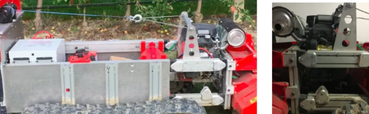
The vehicle is designed for acting in farming environment, performing di↵erent tasks while navigating autonomously. Consequently, for any kind of mission, the robot have to be equipped with proper tools, which, for the sake of modularity, need to be easily plugged or unplugged into the vehicle frame. For this reason, a particular quadrilateral structure have been built in the front of the rover. The latter is composed by two four-bar linkages (see right side of figure 2.4) and has the main feature of having four connecting pins that create the junction between tool and frame. So, the bars composing this structure are not fixed, but can rotate
Figure 2.4: Mechanical system for plugging and managing tools (left) and detail of the quadrilater structure (left).
around their fixing points on the frame, giving the possibility to lift or lower the attached tool. In this way, the tool height can be adjusted to the particular task or
work conditions, also helping the robot during curves or stricht maneuvers, lifting the structure and reducing the ground friction. This mechanism is actuated by an electric winch (see left side of figure 2.4) that, winding or unwinding, makes the four-bar linkage move along vertical direction. Within the above-mentioned mechanism a combustion engine is accommodated, in order to provide mechanical power to the tools mounted onboard. This engine is fed with gasoline (the gas can is visible in figure kjsndf) and generates a power of 40 HP. The mechanical interface between motor and tool is the power take-o↵ used for tractors, meaning that the robot can manage standard agricultural tools, with no need of adaptations or additional components.
2.3
Electrical description
This section describes the electric system of the robot, foundamental for pro-viding motion capacity, winch movements and feeding onboard electronic devices and sensors. The most important components of this subsystem are:
• Lithium batteries • Motors drivers • Motors
• Brakes • Lead battery
• Winch power circuit • DC-DC converters
Batteries are placed in the central part of the robot frame (see figure 2.1), mo-tors and brakes are installed inside tracks structure, while all the other electronic components are mounted on a vertical aluminium plate (see figure 2.6) at the rear of the vehicle, in order to save space and create some kind of heat sink, making it easy for electronic components to disperse heat. Moreover, in this way electric devices are close to the electronic box and wirings and connections are easyer to implement. In the next subsection electric components are described one by one, clarifying both their technical features and functions.
2.3.1
Lithium Batteries
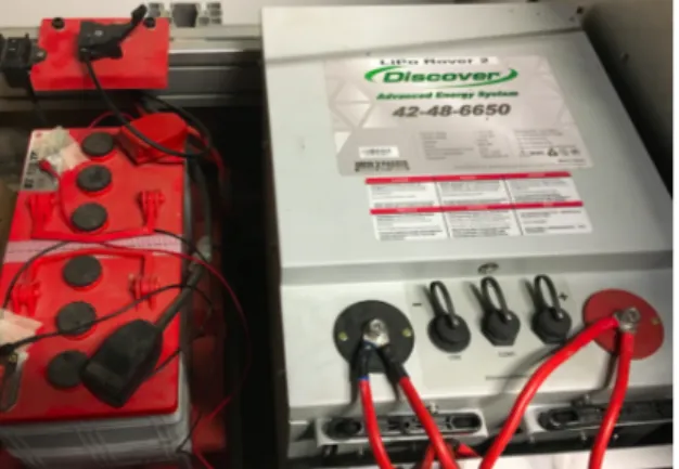
Robot locomotion, electric subsystem and electronics are fed by means of high capacity lithium batteries, which are placed in the central part of the robot frame (see figure 2.5). Most important parameters of these devices are summarized in
Figure 2.5: Detail of lithium and lead batteries installed on the robot.
table 2.1. In the current configuration, the robot is equipped by just one battery, in such a way to test the system in this conditions. After a first experiment session, at least one battery will be added, in order to get an higher autonomy and giving the possibility to feed also the tools and remove the endothermic engine, towards a full electric solution (see chapter 6). From the battery, two parallel connections (two
Parameter Value Nominal voltage 51.2 v Charge voltage 54.4 v Capacity 130 Ah Energy 6656 W h Max. cont. current 130 A Table 2.1: Lithium batteries parameters
negatives and positive poles, for an amount of four cables) goes towards the rear of the vehicle to the aluminium plate, giving 48 v power to motor drivers contactors, to DC-DC converters, and finally to the ignition key. Turning the latter, drivers logic circuit is also fed (see subsection 2.4.2 for further details).
2.3.2
Drivers
This devices are placed on the aluminum plate and have the aim of providing power to the motors, depending on the signals received from the robot controller through the CAN bus connections. Drivers, each one dedicated to a single motor, are fed, in terms of battery power, through the contactors. Figure 2.6 shows a detail of the aluminium plate and components installed on it, during robot construction. In the left upper part is visible the 24 v to 48 v DC-DC, while the other one is already missing, in the central part there are drivers and winch contactors, and in the lower part the two drivers are visible behind wirings. Most important
Figure 2.6: Aluminium plate on which drivers, converters and contactors are installed.
parameters of this devices are summarized in table 2.2. In case of emergency, the
Parameter Value Model Sevcon Size 4 Max. cont. current 180 A (for 60 min.) Spike current 450 A (for 2 min.)
Table 2.2: Drivers parameters
latter can always be switched of from the emergency button (see section 2.4.2), while in nominal situation they are managed by the drivers. Drivers communicate both with the onboard controller, by means of CAN bus and USB-CAN interface (see subsection 2.4.1), and with motors, in terms of power feeding them, and feedback, consisting in motor temperature and encoder signals.
2.3.3
Motors
Motors provide mechanical power to the robot tracks. They are fed, in terms of electric power, by the drivers, and gives back temperature sensor and encoder feed-back, each one to the corresponding controller. Motors most important parameters are summarized in table 2.3.
Parameter Value Model Metalrota PSFBL72 Encoders type sin cos Rated speed 3000 rpm Nominal power 1500 W (for 60 min.) Nominal torque 4.77 N m Nominal current 45 A rms Max torque 16.8 N m (for 25 min.) Max current 135 A (for 5 min.)
Table 2.3: Drivers parameters
2.3.4
Brakes
Brakes are foundamental for safety, in order to avoid risks when operating in robot proximity or to stop it in case of emergency. Brakes are fed at 24 v power, coming from the 48 v to 24 v DC-DC and controlled by ignition key and emergency button (see section 2.4.2). Of course, when the circuit, namely a coil, is switched o↵, brakes are active, in the sense that they keep the robot tracks stuck, and viceversa if the circuit is alive.
2.3.5
DC-DC Converters
A couple of DC-DC converters is placed on the aluminium plate (see figure 2.6), with the aim of providing proper voltage power to sensors, brakes and electronics, which works at a lower voltage level than the batteries one. In particular, a 48 v to 24 v converter feed brakes and microcontrollers, through a small 24 v to 5 v device, while a 48 v to 12 v one provides power to sensors and onboard computer. The first converter gives a maximum current of 8.3 A, at 24 v, while the second can provide 16 A, of course at 12 v.
2.3.6
Lead Battery
Close to the lithium battery, also a lead one is installed (see left side of figure 2.5), with the aim of:
- Switch on the endothermic engine (see subsection 2.2.3) - Feed the winch, for tools height regulation (2.2.3)
This device is actually a common car lead battery, working at a nominal voltage of 12 v and 120 Ah stored energy.
2.3.7
Winch Circuit
The winch mounted at the rear of the vehicle works at 12 v and absorbs, as maximum value, a current of 130 A. For this reason, it has not been possible to feed this device through a DC-DC, exploiting lithium batteries already installed onboard, and in the current robot configuration it is connected to the lead battery. The winch is managed by means of a contactor, which makes it lift or lower based on its control switch position (visible in the upper left corner of figure 2.5). Ac-tually, the winch can be manually operated by means of a switch placed close to the lead battery, but also remotely controlled. In this case, joypad commands (see subsection 2.4.4) triggers two relays of the electronic box (through NUC and ar-duino Mini Pro microcontroller), which in turns act on the winch contactor. This funtion is useful for adapting the tool height while manually driving the robot, without breaks or need to reach the manual switch.
2.4
Electronic Box and Sensors
This section describes the third subsystem composing the robot structure, i.e. electronics and onboard sensors. In the next subsection (2.4.1) the electronic box is presented, which contains all components providing for robot control and sensors reading. Finally, in subsection 2.4.3, sensors installed on the robot are described.
2.4.1
Electronic Box
The electronic box has the aim of controlling the robot and contains all the components necessary for providing this service. The most important box functions
are summarized in the list below.
• Manage low voltage power, i.e. 12 v and 24 v, which must be provided to the di↵erent electronic components.
• Sensor management, in terms of power supply and reading • Brakes management
• Run onboard computer applications, i.e. user interface and autonomous navigation algorithm
• Deal with the manual controller
• Communicate with motors drivers, sending references and receiving feedback • Guarantee a certain safety level for humans dealing with the robot, by means
of manual buttons
Figure 2.7 shows a view of the panels and components of the electronic box. The lower panel is quite hidden, while on the upper one are visible an ethernet switch, the LIDAR board, an Arduino Mini Pro and a Mega 2560 microcontrollers. Here
Figure 2.7: View of the whole content of the electronic box.
below the electronic box components are presented and described, focusing on their function, in such a way to give a complete discussion about both electronic devices contained in the box and related service they supply.
Intel NUC
This is the onboard controller of the robot and runs all the code which provides user interfacement and autonomous navigation capabilities. For thi function, an Intel NUC has been chosen, a compact mini-PC highly customizable that ensures good computational power in a quite limited footprint. For what concerns the application, among the countless models available on the market it has been chosen the D54250WYKH, this choice is motivated by the fact that, at the beginning of the project it was one of the best option with respect to the price/performance ratio. The key advantage of having a PC onboard is the possibility of having
Figure 2.8: Intel NUC model D54250WYKH, external and inner view.
Operating Systems running onboard, endowing the system with an extremely high versatility. Furthermore, by means of virtual machines it’s possible to use di↵erent OSs. Indeed, in the developed software structure the operating systems installed onboard are:
• Windows 7, for user interfacement features
• Linux Ubuntu, for autonomous navigation implementation
In chapter 4 a detailed view of the software structure inside the onboard pc is given, but it is important to highlight some aspects also in this section, in order
to better understand the presence of some hardware items.
The part running Windows is devoted to interface the user with the machine and to receive commands and feedbacks from the navigation algorithm and in turn send them to the motor drivers.
The Windows-running machine is connected, via USB, to the following devices: - Arduino Pro Mini
- IXXAT Can Interface
On the other hand, software running under the Ubuntu Operating System permits to communicate with sensors. Therefore the Linux Ubuntu machine is connected, both via USB and Ethernet port, to:
- Arduino Mega 2560 (USB)
- Velodyne LIDAR PUCK VLP-16 (Ethernet) - Trimble R8s GNSS System (USB)
As can be seen in the lists above, the two operating systems are connected to their own Arduino board. This choice has been taken in order to create an organized communication structure, in which an Arduino, plugged to the Windows part, is aimed to control peripheral devices or functionalities directly from HMI commands, and the other one, connected to Ubuntu, with the task of reading data from sensors. Of course the NUC is connected to a power source, at 12 v, and to a screen, a 10,1 inches screen with touch-screen features. This characteristic ensures an higher level of convenience than using mouse/keyboard away from the desktop and make it easy to deal with the pc even during experiments within orchards.
Arduino Pro Mini
Arduino Pro Mini microcontroller, showed in figure 2.9, communicates with the robot HMI, receiving user commands and sending him some feedback. In particular, it controls:
- Array of relays, in order to provide power and activate sensors or other components
- Electronic box cooling fans
On the other side, it provides feedback about relays conditions, indicating if a device is active or not, and temperature inside the electronic box. This latter information is also used, by the microcontroller, for regulating the cooling fans
and keeping it within a safety threshold. These feedback are proposed to the user in the first screen of the robot HMI (see figure 4.2).
Figure 2.9: Arduino Pro Mini microcontroller.
Relays array
This Arduino module is composed by an array of eight relays whose coils are opto-isolated (see figure 2.10). Therefore, it can be directly connected to the Arduino board without any worry about safety. In order to avoid malfunctions or saturations, coils activation currents are provided by the power supply, at a 5 v level, and do not come from the Arduino pins, whose capacity is limited to about 100 mA.
This module is used to supply power to several devices, which are not required
Figure 2.10: Arduino relay module.
to keep enabled if not used:
• Ethernet Switch, used to increase the number of possible Ethernet connec-tions, since the NUC has just one RJ45 port, and it needs to be connected
to the LIDAR, to the virtual machine and to the internet network.
• LIDAR VLP-16, which is foundamental for autonomus navigation experi-ments, but can be switched o↵, for saving batteries, during debug or when the robot is manually driven.
• Motor Brakes, which needs to be armed and disarmed depending whether the robot has to move or not. Brakes managements through the microcon-troller gives the possibility to remotely activate or deactivate brakes, from the Arduino or the HMI.
Cooling Fans and Temperature Sensor
Within the electronic box there are many components (mainly the NUC mini PC) that emits a lot of heat, which is not healthy for the electronics function-ing. Therefore, a system for controlling the box temperature has been designed. A DTH22 temperature sensor (see right side of figure 2.11) is connected to the
Figure 2.11: Cooling system of the electronic box, composed by cooling fans (left side) and temperature sensor (right side)
Arduino Pro Mini. On the basis of sensor data, the microcontroller regulates the spinning velocity of two cooling fans (left side of figure 2.11), in order to keep the temperature box within a safety range. The two cooling fans are attached onto the box in such a way to have one blowing inside cooler air, and the other one pushing out the hotter air. Moreover, powder filters has been mounted both onto the inlet fan, in order to avoid aspiration of undesired and potentially dangerous elements, and onto the outlet fan, to avoid the entrance of particles when the fan is standing still).
Arduino Mega 2650
The Arduino Mega microcontroller (see figure 2.12) is connected to the Ubuntu operating system and reads data coming from low-cost GPS, with a built-in magne-tometer, and exchanges data through a serial communication channel with another Arduino Pro Mini. The latter is directly connected with an Inertial Measurement
Figure 2.12: Arduino Mega 2650.
Unit (IMU) through an IIC (I2C) bus. This solution could appear quite strage, but it is motivated by two factors:
- The IMU has been placed really close to the center of gravity, in order to make it easy to read and interpret its measurements, even if it means to mount it far from the electronic box, and close to batteries and power cables, i.e. expose it to high electromagnetic fields.
• The IMU interface consists in a I2C bus, which is really sensitive to EM disturbances.
For this reason, the IMU has been connected to an Arduino Mini, placed really close to it, in order to keep I2C wires as short as possible and be less sensitive to environment disturbances. Sensor measurents are sent via serial communication, which is more robust, to the Arduino Mega board, which transmit these data to the onboard pc.
IXXAT Can Interface
In section 2.3 motors electric drives has been described, discussing about their CAN communication protocol, used for comminicating with external devices. Of course an interface is needed, in order to provide communication between onboard pc and CAN side. The chosen USB-CAN interface (see figure 2.13) has the burden of converting signals from an USB port that is plugged into the NUC and a 9-pin connector which implements the CAN-bus, and viceversa.
Figure 2.13: IXXAT USB-CAN Interface.
2.4.2
Buttons Panel
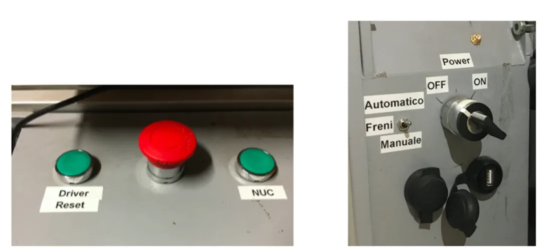
On the external part of the electronic box are installed some manual buttons or switches, which provide to the system additional functionalities. Figure 2.14 shows a view of top and right side of the box (at left and right sides of the picture, respectively), on which those items are placed. Here below these buttons are listed and described, focusing on the features or safety function they provide
• Ignition key
Placed on the right side of the electronic box, has the function of switching on, or o↵, the whole electronic subsystem of the robot. In particular, the key interrupts:
- 12 v power, coming from the 48 v to 12 v DC-DC, which supply the onboard computer, sensors and microcontrollers.