Elements of Concurrent Programming
Third Edition
Preface . . . 1
1. Deterministic Computations . . . 3
1.1 Operational Semantics of Arithmetic Expressions . . . 3
1.2 Operational Semantics of Boolean Expressions . . . 3
1.3 Operational Semantics of Commands . . . 4
2. Nondeterministic Computations (Big Step Semantics) . . . 5
2.1 Operational Semantics of Nondeterministic Commands . . . 5
2.2 Operational Semantics of Guarded Commands . . . 6
3. Concurrent Programs: Vectorization . . . 7
3.1 Process Declaration and Process Call . . . 7
3.2 Concurrency Based on Vectorization Using fork-join . . . 7
3.3 Concurrency Based on Vectorization Using cobegin-coend . . . 9
3.4 Example: Evaluating Recurrence Relations . . . 10
3.5 Example: Multiplying Matrices . . . 11
4. Concurrent Programs Based on Shared Variables . . . 12
4.1 Preliminary Example: Prefix Sums . . . 12
4.2 Prefix Sums Revisited . . . 13
4.3 Semaphores . . . 17
4.4 Semaphores and Test-and-Set Operations for Mutual Exclusion . . . 19
4.5 Semaphores for Mutual Exclusion for Producers and Consumers . . . 20
4.6 Private Semaphores for Establishing a Policy to Resume Processes . . . 22
4.7 Critical Regions and Conditional Critical Regions . . . 26
4.8 Monitors . . . 31
4.9 Using Monitors for Solving the Five Philosophers Problem . . . 36
4.10 Using Semaphores for Solving the Five Philosophers Problem . . . 39
4.11 Peterson’s Algorithm for Mutual Exclusion . . . 42
4.12 Distributed Computation of Spanning Trees . . . 51
4.13 Distributed Termination Detection . . . 58
4.14 Lock-free and Wait-free Synchronization . . . 63
5. Concurrent Computations in Java . . . 64
5.1 Mutual Exclusion in Java . . . 67
5.2 Monitors in Java . . . 70
5.3 Bounded Buffer Monitor in Java . . . 73
5.5 Binary Semaphore in Java . . . 77
5.6 Bounded Buffer with Binary and Counting Semaphores in Java . . . 77
5.7 Five Philosophers Problem in Java . . . 80
5.8 Queue Monitor in Java . . . 82
6. Concurrent Programs Based on Handshaking Communications . . . 85
6.1 Pure CCS Calculus . . . 85
6.2 Verifying Peterson’s Algorithm for Mutual Exclusion . . . 89
6.3 Value-Passing CCS Calculus . . . 94
6.4 Verifying the Alternating Bit Protocol . . . 96
7. Transactions and Serializability on Databases . . . 101
7.1 Preliminaries . . . 101
7.2 SerializabilityTheory . . . 103
7.3 An Abstract View of Transactions . . . 103
7.4 Histories and Equivalent Histories . . . 106
7.5 The Serializability Theorem . . . 108
7.6 Locking Protocols . . . 109
7.7 Two Phase Locking Protocols . . . 112
7.8 Strict Two Phase Locking Protocols . . . 113
7.9 Deadlocks . . . 114
7.10 Conservative Two Phase Locking Protocols . . . 115
7. Appendix: A Distributed Program for Computing Spanning Trees . . 116
Index . . . 129
These lecture notes are intended to introduce the reader to the basic notions of nonde-terministic and concurrent programming. We start by giving the operational semantics of a simple deterministic language and the operational semantics of a simple nondetermin-istic language based on guarded commands. Then we consider concurrent computations based on: (i) vectorization, (ii) shared variables, and (iii) handshaking communications à la CCS (Calculus for Communicating Systems) [16]. We also address the problem of mu-tual exclusion and for its solution we analyze various techniques such as those based on semaphores, critical regions, conditional critical regions, and monitors. Finally, we study the problem of detecting distributed termination and the problem of the serializability of database transactions.
Sections 1, 2, and 6 are based on [16,22]. The material of Sections 3 and 4 is derived from [1,2,4,5,7,8,13,18,20]. Section 5 is based on [10] and is devoted to programming examples written in Java where the reader may see in action some of the basic techniques described in these lecture notes. In Section 7 we closely follow [3].
We would like to thank Dr. Maurizio Proietti for his many suggestions and his en-couragement, Prof. Robin Milner and Prof. Matthew Hennessy for introducing me to CCS, Prof. Vijay K. Garg from whose book [10] I learnt concurrent programming in Java, my colleagues at Roma Tor Vergata University for their support and friendship, and my students for their patience and help.
Many thanks also to Dr. Gioacchino Onorati and Lorenzo Costantini of the Aracne Publishing Company for their kind and helpful cooperation.
Roma, April 2005
In the third edition we have corrected a few mistakes, we have improved Chapter 2, and we have added in the Appendix a Java program for the distributed computation of spanning trees of undirected graphs. Thanks to Dr. Emanuele De Angelis for discovering an error in the presentation of Peterson’s algorithm.
Roma, January 2009 Alberto Pettorossi
Department of Informatics, Systems, and Production University of Roma Tor Vergata
Via del Politecnico 1, I-00133 Roma, Italy email: [email protected] URL: http://www.iasi.cnr.it/~adp
1
Deterministic Computations
We begin by considering deterministic computations such as those denoted by a simple Pascal-like language. In this language we have the following syntactic categories:
- Integers
n, m, . . . range over Z = {. . . , −2, −1, 0, 1, 2, . . .} - Locations (or memory addresses)
X, Y, . . . range over Loc - Arithmetic Expressions
a ranges over AExpr a ::= n | X | a1+ a2 | a1− a2 | a1× a2
- Boolean Expressions
b ranges over BExpr b ::= true | false | a1 = a2 | a1 ≤ a2 | ¬b | b1∨ b2 | b1∧ b2
- Commands
c ranges over Com c ::= skip | X := a | c1; c2 | if b then c1else c2 | while b do c
Below we introduce the operational semantics of our Pascal-like language. The operational semantics specifies:
- the evaluation of arithmetical expressions, - the evaluation of boolean expressions, and - the execution of commands.
In order to specify the operational semantics we need the notion of a state. A state σ is a function from Loc to Z. The set of all states is called State. 1.1 Operational Semantics of Arithmetic Expressions
The evaluation of arithmetic expressions is given as a subset of AExpr × State × Z. A triple in AExpr × State × Z is written as &a, σ' → n and specifies that the arithmetic expression a in the state σ evaluates to the integer n. The axioms and the inference rule defining the evaluation of arithmetic expressions are as follows.
&n, σ' → n &X, σ' → σ(X)
&a1,σ' → n1 &a2,σ' → n2
&a1opa2, σ' → n1op n2
where op ∈ {+, −, ×} and op is the semantic operation corresponding to op.
1.2 Operational Semantics of Boolean Expressions
The evaluation of boolean expressions is given as a subset of BExpr ×State ×{true, false}. A triple in BExpr × State × {true, false} is written as &b, σ' → t and specifies that the boolean expression b in the state σ evaluates to the boolean value t. The axioms and the inference rules defining the evaluation of boolean expressions are as follows.
&true, σ' → true &false, σ' → false &a1,σ' → n1 &a2,σ' → n2 &a1=a2, σ' → true if n1 = n2 &a1,σ' → n1 &a2,σ' → n2 &a1=a2, σ' → false if n1 *= n2 &a1,σ' → n1 &a2,σ' → n2 &a1≤ a2, σ' → true if n1 ≤ n2 &a1,σ' → n1 &a2,σ' → n2 &a1≤ a2, σ' → false if n1 *≤ n2 &b,σ' → true &¬b,σ' → false &b,σ' → false &¬b,σ' → true &b1,σ' → t1 &b2,σ' → t2
&b1bopb2, σ' → t1bop t2
where bop ∈ {∨, ∧} and bop is the semantic operation corresponding to bop.
1.3 Operational Semantics of Commands
We need the following notation. By σ[n/X] we mean the function which is equal to σ except in X, where it takes the value n, that is:
σ[n/X] (Y ) = !
n if Y = X σ(Y ) if Y *= X
The execution of commands is given as a subset of Com × State × State. A triple in Com × State × State is written as &c, σ' → σ! and specifies that the command c from
the state σ produces the new state σ!. The axiom and the inference rules defining the
execution of commands are as follows. &skip, σ' → σ
&a,σ' → n &X:=a, σ' → σ[n/X] &c1,σ' → σ1 &c2,σ1' → σ2
&c1;c2, σ' → σ2
&b,σ' → true &c1,σ' → σ1 &if b then c1else c2, σ' → σ1
&b,σ' → false &c2,σ' → σ2 &if b then c1else c2, σ' → σ2 &b,σ' → false
&while b do c, σ' → σ
&b,σ' → true &c,σ' → σ1 &while b do c, σ1' → σ∗
&while b do c, σ' → σ∗
Note 1. The ternary operator &_, _' → _ is overloaded and it is used for the operational semantics of arithmetic expressions, boolean expressions, and commands.
Here is Euclid’s algorithm for computing the greatest common divisor of M and N using commands (we assume that M > 0 and N > 0):
{n = N > 0 ∧ m = M > 0}
while m *= n do if m > n then m := m−n else n := n−m od {gcd(N, M) = n}
2
Nondeterministic Computations (Big Step Semantics)
We present the guarded commands first introduced by Dijkstra [9]. They allow non-deterministic computations. We have the following new syntactic categories (which are mutually recursively defined):
- Commands
c ranges over Com c ::= skip | abort | X := a | c1; c2 | if gc fi | do gc od
- Guarded Commands
gc ranges over GCom gc ::= b → c | gc1 gc2
where a ranges over the arithmetic expressions AExpr and b ranges over the boolean expressions BExpr. The operator is assumed to be associative and commutative. The operational semantics given below specifies:
- the execution of commands and - the execution of guarded commands.
2.1 Operational Semantics of Nondeterministic Commands
The execution of commands is given as a subset of Com × State × State. A triple in Com × State × State is written as &c, σ' → γ and specifies that the command c from the state σ produces the new state γ. The axiom and the inference rules defining the execution of commands are as follows.
(1.1) &skip, σ' → σ
(1.2) &X:=a, σ' → σ[n/X]&a,σ' → n
(1.3) &c1,σ' → σ&c 1 &c2,σ1' → σ2
1; c2, σ' → σ2
(1.4) &gc,σ' → &c,σ' &c,σ' → σ
,
&if gc fi, σ' → σ,
(1.5) &do gc od, σ' → σ&gc,σ' → fail (1.6) &gc,σ' → &c,σ' &c; do gc od, σ' → σ
,
&do gc od, σ' → σ, Let us informally explain the rules for the if . . . fi and do . . . od commands.
The execution of if gc1 . . . gcnfi is performed as follows.
(i) We first choose in a nondeterministic way a guarded command, say b → c, among gc1, . . . , gcn, such that the guard b evaluates to true, and then
(ii) we execute the command c.
(iii) If no guarded command among {gc1, . . . , gcn} has a guard which evaluates to true,
the execution of the if . . . fi command is aborted, and the execution of the whole program is aborted.
The execution of do gc1 . . . gcnod is performed as follows.
(i) We first choose in a nondeterministic way a guarded command, say b → c, among {gc1, . . . , gcn} such that the guard b evaluates to true, then
(ii) we execute the command c and then go to Step (i).
(iii) If no guarded command among gc1, . . . , gcn, has a guard which evaluates to true, the
execution of the do . . . od command is terminated and the execution continues with that of the command following the do . . . od command.
Note that we gave no rules for the command abort. Thus, for every state σ ∈ State and every γ ∈ State no triple &abort, σ, γ' exists in the subset of Com × State × State which denotes the operational semantics.
2.2 Operational Semantics of Guarded Commands
The execution of guarded commands is given as a subset of GCom × State × ((Com × State) ∪ {fail}). A triple in GCom × State × ((Com × State) ∪ {fail}) is written as &gc, σ' → γ and specifies that the guarded command gc from the state σ produces either the new &command, state' pair γ or the value γ = fail. The inference rules defining the execution of guarded commands are as follows.
(2.1) &b→c, σ' → &c,σ'&b,σ' → true (2.2) &b → c, σ' → fail&b,σ' → false (2.3) &gc&gc1,σ' → &c,σ'
1 gc2, σ' → &c,σ' (2.4)
&gc2,σ' → &c,σ' &gc1 gc2, σ' → &c,σ' (2.5) &gc1, σ' → fail&gc &gc2, σ' → fail
1 gc2, σ' → fail
Note that when evaluating the guard of a guarded command, the state is not changed. This fact is not exploited in the semantic rules given by Winskel [22].
Instead of the above rules (2.3) and (2.4), we can equivalently use the following two rules:
(2.3*) &b→c gc&b→c,σ' → &c,σ'
2, σ' → &c,σ' (2.4*)
&b→c,σ' → &c,σ' &gc1 b→c, σ' → &c,σ' Note also that for all b, c, σ, gc1, gc2, we have that:
(i) &b → c, σ' → &c, σ' holds iff &b, σ' → true, and
(ii) &gc1 gc2, σ' → &c, σ' holds iff there exists i ∈ {1, 2} such that gci is b → c and &b, σ' → true.
Here is Euclid’s algorithm for computing the greatest common divisor of M and N using guarded commands (we assume that M > 0 and N > 0):
{n = N > 0 ∧ m = M > 0} do m ≥ n ∧ n > 0 → m := m−n
n ≥ m ∧ m > 0 → n := n−m od
{gcd(N, M) = if n = 0 then m else n}
The assertions between curly brackets at the beginning and at the end of the above do . . . od command relate the value of the integer variables before and after the execution of that command.
3
Concurrent Programs: Vectorization
The terminology about concurrent programming is not stable. Some authors consider concurrent programs, distributed programs, and parallel programs to be the same class of programs. Other authors do not.
We assume three forms of concurrency: (i) concurrency based on vectorization,
(ii) concurrency based on shared variables (and shared resources), and
(iii) concurrency based on handshaking communications (also called rendez-vous). With respect to sequential programs the use of concurrent programs allows us: (i) to get better performance, and (ii) to simulate in a direct way concurrent processes (or agents) which perform computations in real world systems.
3.1 Process Declaration and Process Call
Process declarations and process calls in parallel languages are like procedure declarations and procedure calls in sequential languages, but the called processes run together with the calling processes.
In Concurrent Pascal [5] and Modula [23,24] process declaration can be done at top level only. In this case we say that the processes are static.
In Ada [17] a process declaration can be inside an enclosing process declaration. In this case we say that the processes are dynamic.
3.2 Concurrency Based on Vectorization Using fork-join
The fork-join construct was introduced in [7]. We describe here the following two variants: (1) single fork-join, and (2) multiple fork-join.
(1) Single fork-join:
(Process A) A: (a0)
fork B −→ (Process B ) B : (start)
↓ ↓
(a1) (b)
↓ ↓
JB: join B ←− go to JB (a2)
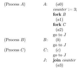
(2) Multiple fork-join: (Process A) A: (a0) counter := 3; fork B (a1) fork C (a2) go to J (Process B) B: (b) go to J (Process C) C: (c) go to J J: join counter (a3)
Process A proceeds after the instruction join counter, when both process B and process C have terminated.
Multiple fork-join is used, for example, when one has to sum two arrays, say A1 and
A2, of N elements each, and N is a large number. The sum can be done in parallel by
k processes, each summing N/k elements (we assume that N/k is an integer). These k processes are generated by a k-fold fork. In particular, process 1 sums the elements of the arrays A1 and A2 from position 0 to position (N/k) − 1, ..., and process k sums the
elements of the arrays A1 and A2 from position N − (N/k) to position N − 1.
With every fork-join program we can associate a multigraph, called control flow multigraph, whose nodes are the fork and join instructions and whose arcs connect nodes according to the usual notion of control flow for sequential programs. (We assume that the reader is familiar with this notion.) Note that we consider a multigraph, instead of a graph, because parallel execution may determine two or more arcs between two nodes. For example, the multigraph corresponding to the above program with processes A, B, and C, is depicted in the following Figure 1.
! ! " # $ " # # (a1) (a2) fork B % fork C % %join counter (b) (c)
Fig. 1. A control flow multigraph.
The computation continues after a join node n iff the computation relative to every arc arriving at n is terminated.
With every control flow multigraph we associate a relation, denoted ≤, induced by its arcs. For instance, in the multigraph of Figure 1 we have that: fork C ≤ join counter, fork B ≤ fork C, and fork B ≤ join counter. If a1≤ . . . ≤ an, for some n ≥ 0, we say
that a1 is an ancestor of an or, equivalently, an is a descendant of a1. In particular, any
node a is an ancestor and a descendant of itself.
3.3 Concurrency Based on Vectorization Using cobegin-coend
The cobegin-coend command was introduced in [8]. It has the following syntax: cobegin S1; ...; Sn coend
Its execution activates n processes, say P1, . . . , Pn. Process P1 executes statement S1, ...,
and process Pn executes statement Sn. The cobegin-coend command terminates when
all processes have terminated.
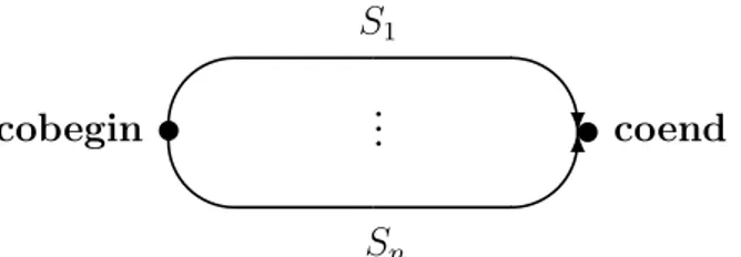
We assume that every cobegin S1; ...; Sn coend command generates a control flow
multigraph such as the one depicted in Figure 2.
! ! " # $ " % %
.
.
.
Sn S1 cobegin coendFig. 2. The control flow multigraph generated by the cobegin S1; ...; Sncoend command.
Not all control flow multigraphs that can be generated by fork-join constructs (together with sequentialization, if-then-else, and while-do constructs), can also be generated by cobegin-coend commands (together with sequentialization, if-then-else, and while-do constructs). Obviously, in this generation we consider only the topology of the multigraphs and not the labels of the nodes.
For instance, the multigraph depicted in Figure 3, generated by the program PABC
which consists of the following three processes A, B, and C, cannot be generated by cobegin-coend commands. (Process A) A: (a0) fork B (a1) fork C (a2) JB: join B (a3) JC: join C go to J (Process B) B: (b) go to JB (Process C) C: (c) go to JC J: (a4)
! ! " # $ " # # #
(a1) (a2) (a3) fork B % (b) fork C % JB% (c) JC %
Fig. 3. The control flow multigraph generated by the program PABC.
Let us consider the following Property ∆ of a control flow multigraph:
Property ∆: given any two nodes n1 and n2, every descendant of the least common
ancestor of n1 and n2, is predecessor or a descendant of the greatest common successor of
n1 and n2.
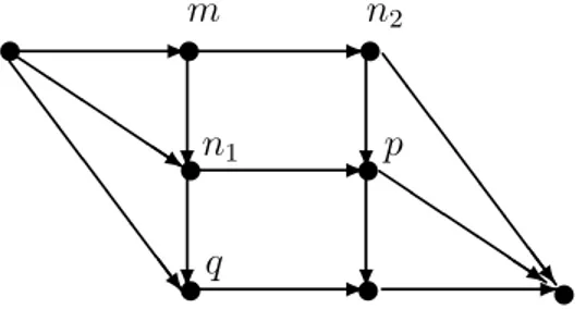
We have that if a control flow multigraph can be generated by using cobegin-coend commands then it satisfies Property ∆. A multigraph which does not satisfy Property ∆ (and therefore, it cannot be generated by using cobegin-coend commands), is the one depicted in Figure 4. Indeed, in Figure 4 node q which is a descendant of the least common ancestor m of the nodes n1 and n2, is neither a predecessor nor a descendant of the node p
which is the greatest common successor of n1 and n2.
Notice that Property ∆ is a necessary condition for a control flow multigraph to be generated by using cobegin-coend commands, but it is not a sufficient condition, as shown by the multigraph of Figure 3.
% % % % % % % % ! #! # # ! #! # $$ $$ $$% $$ $$ $$% & & & & & & &&' & & & & & & &&' m n1 n2 p q
Fig. 4. A control flow multigraph which cannot be generated by using cobegin-coend commands.
3.4 Example: Evaluating Recurrence Relations
In order to compute recursive programs which are not linear recursive we can compute in parallel the m (> 1) recursive calls. For instance, for the Fibonacci numbers we have:
procedure fibonacci(int n, int f ); begin if n ≤ 1 then f := 1 else
begin cobegin fibonacci(n−1, f 1); fibonacci(n−2, f 2) coend; f := f 1 + f 2
end end
3.5 Example: Multiplying Matrices
Given the following two n × n matrices A and B such that A = " " " "AA1121AA1222 " " " " and B = " " " "BB1121BB1222 " " " ", we have that C = " " " "CC1121CC1222 " " " " is the product A × B iff C11 = A11×B11+ A12×B21, C12= A11×B12+ A12×B22, C21 = A21×B11+ A22×B21, C22= A21×B12+ A22×B22.
Thus, we can compute C by performing in parallel 8 multiplications of n/2 × n/2 matrices as follows. For reasons of simplicity we assume that n is a power of 2.
procedure mult(int n, int A[1..n, 1..n], int B[1..n, 1..n], int C[1..n, 1..n]); begin if n = 1 then C := A × B else
begin cobegin mult(n/2, A11, B11, C1); mult(n/2, A12, B21, C2); mult(n/2, A11, B12, C3); mult(n/2, A12, B22, C4); mult(n/2, A21, B11, C5); mult(n/2, A22, B21, C6); mult(n/2, A21, B12, C7); mult(n/2, A22, B22, C8) coend; cobegin C11 := C1 + C2; C 12 := C3 + C4; C21 := C5 + C6; C 22 := C7 + C8 coend; C := arrange(C11, C12, C21, C22) end end
where arrange is a function that given four n/2 × n/2 matrices, say C11, C12, C21, and C22, constructs the n×n matrix C =
" " " "C11 C12C21 C22 " " " ".
4
Concurrent Programs Based on Shared Variables
4.1 Preliminary Example: Prefix Sums
Let us present a preliminary example of a concurrent program based on shared variables. We are given a sequence &x0, x1, . . . , xn−1' of n numbers and we want to compute the
sequence &s0, s1, . . . , sn−1' also of n numbers such that:
s0 = x0,
s1 = x0 + x1,
s2 = x0 + x1+ x2, . . ., and
sn−1 = x0+ x1+ . . . + xn−1.
This computation can be performed by the following program, where we assume n pro-cessors P0, P1, . . . , Pn−1. For i = 0, 1, . . . , n−1, processor Pi initially holds xi and, finally,
Pi holds si. To make subscripts more readable we write 2∧t, instead of 2t.
par-for i = 0 to n − 1 do si := xi od;
for t = 0 to (log n) − 1 do
par-for k = 2∧t to n − 1 do s
k := sk+ sk−2∧t od (†)
od In this program the construct
par-for i = 0 to p do bodyi od
is executed by making every processor Pi, for i = 0, . . . , p, to execute bodyi independently
and in parallel. The statement terminates when all processors have terminated. Thus, in line (†) above the values of sk and sk−2∧t in the expression sk+ sk−2∧t are the results of
the previous iteration of the par-for loop of the same line (†). In general: par-for i = 1 to p do bodyi od
is assumed to be equivalent to:
cobegin body1 ; . . .; bodyp coend.
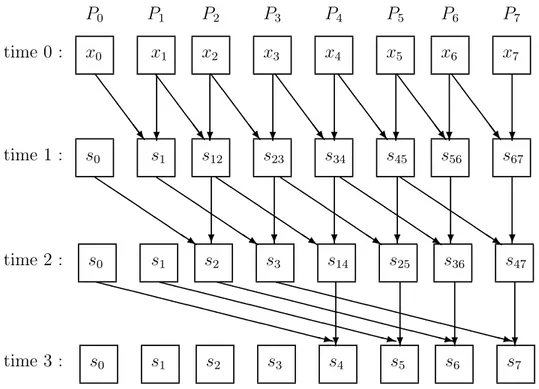
The above program uses the so called recursive doubling technique. This name comes from the fact that the number of processors which have no sums to perform, doubles at each execution of the body of the outermost par-for loop. The flow of data, when n = 8, is depicted as in Figure 5. There are 8 processors, one for each column. Each row shows the value computed by the processors at the corresponding time. Values arriving at a processor along incoming arcs are added together, and copies of the results are sent along the outgoing arcs.
The complexity or cost of the above program measured in time × number of processors is O(log n)×O(n), i.e., O(n log n). This cost is not optimal because if we use one processor only, the time × number of processors complexity is O(n) × O(1), that is, O(n).
Notice that the above program which is used for summing up the numbers of a se-quence, can also be used for computing the sequence &p0, p1, . . . , pn−1' of products such
that: p0 = x0, p1 = x0×x1, . . ., and pn−1 = x0×x1×. . .×xn−1, by replacing sk := sk+ sk−2∧t
bysk := sk× sk−2∧t. Indeed, that program can be used for any binary operation which is
! ! ! ! ! ! ! & & & &&' & & & &&' & & & &&' & & & &&' & & & &&' & & & &&' & & & &&' ! ! ! ! ! ! $$ $$ $ $$% $$ $$ $ $$% $$ $$ $ $$% $$ $$ $ $$% $$ $$ $ $$% $$ $$ $ $$% ! ! ! ! ((((( ((((( (((((() ((((( ((((( (((((() ((((( ((((( (((((() ((((( ((((( (((((() P0 P1 P2 P3 P4 P5 P6 P7 time 0 : time 1 : time 2 : time 3 : x0 x1 x2 x3 x4 x5 x6 x7 s0 s1 s12 s23 s34 s45 s56 s67 s0 s1 s2 s3 s14 s25 s36 s47 s0 s1 s2 s3 s4 s5 s6 s7
Fig. 5. The computation of prefix sums of the 8 numbers: x0, x1, . . ., x7. For 0 ≤ i ≤ 7,
si denotes x0+ x1+ . . . + xi. s0 = x0. For 0 ≤ i ≤ j ≤ 7, sij denotes xi+ xi+1+ . . . + xj.
Finally, let us notice that sometimes the distinction between concurrent computations which are based on vectorization and those which are based on shared memory is not so sharp. Indeed, this distinction very much depends on the amount of interactions among the various processes (or processors) during the execution of the bodies of the par-for loops involved in the computation. If there is little interaction, we prefer to say that the computation is based on vectorization, otherwise, we say that it is based on shared memory.
4.2 Prefix Sums Revisited
Let us consider again the example of the previous Section 4.1. We will present two new programs for the computation of the prefix sums of a given sequence x0, . . . , xn−1 of n
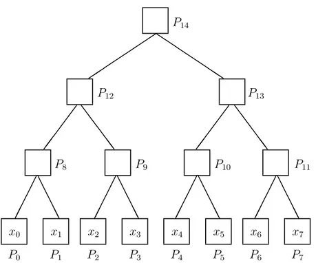
numbers. Both programs run on a tree of processors (see also Figure 6 where we consider the case for n = 8), but they have different complexity measured in terms of time × num-ber of processors. The first program has O(n log n) complexity (which is not optimal), while the second program has O(n) complexity (which is optimal). The optimal complex-ity is O(n) because every program should look at every number of the sequence and the length of the sequence is n.
Let us consider the first program P 1. We assume that we have n processors P0, . . .,
Pn−1, each one at a leaf of a binary tree of processors, and we also have n − 1 processors,
P0 P1 P2 P3 P4 P5 P6 P7 * * * * * * * $$ $$ $ $$ & & & && + + + + + & & & && + + + + + , , , ,, - --, , , ,, - --, , , ,, - --, , , ,, - --x0 x1 x2 x3 x4 x5 x6 x7 P8 P9 P10 P11 P12 P13 P14
Fig. 6. The computation of prefix sums of a sequence x0, . . . , x7 of n (= 8) numbers on a
tree of 2n−1 (= 15) processors: P0, . . . , P14.
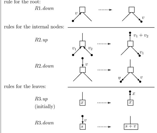
n is a power of 2 (see Figure 6 where n = 8). The parallel computation proceeds according to the following rules (see also Figure 7) in an asynchronous way, that is, a rule is applied in a node of the tree whenever it can be applied, regardless at what happens in other nodes:
- rule for the root:
Rule R1.down: the root, after receiving a value v from its left child, sends v to the right child;
- rules for the internal nodes:
Rule R2.up: an internal node, after receiving the values v1 and v2 from its children,
sends their sum v1+ v2 to the father and sends the value v1 from the left child to the right
child;
Rule R2.down: an internal node, after receiving a value v from its father, sends v to the two children;
- rules for the leaves:
Rule R3.up: a leaf sends its value x to its father, and this operation is performed only once at the beginning of the computation;
Rule R3.down: a leaf, after receiving a value v from its father, sums v to its own value. Notice that throughout the computation: (i) one value only is received by the root and this value is the only value sent by the root down to its children, (ii) one value only is sent up by any non-root node to its father, and (iii) one value only is sent down by any non-leaf node to its children.
. . . ///0 & /// ...1& # # # # # /// ... ! & / / / 2 & ...1& ! & /// ...1& ///0 & ..3.& " & " & v v rule for the root:
R1.down v1 v2 v1+ v2 R2.down v vv v
rules for the leaves:
x
R3.down
s v
s + v rules for the internal nodes:
v1
R2.up
R3.up
(initially) x x
Fig. 7. The rules for the computation of prefix sums for Program P 1. The initial value of s is x. The rule for the root is an instance of the rules for the internal nodes, because the root has no father.
The time taken by this program is O(log n) because a value has to travel up to the root and then down to the leaves. The number of processors is 2n−1. Thus, the time × number of processors complexity is O(n log n).
Now we present a second program P 2 for the computation of the prefix sums. This program P 2 is like program P 1, except that the rules for the computation at the leaves are modified.
We assume that we are given a sequence of n numbers, and we have N processors, named P0, . . . .PN−1, placed at the N leaves of the binary tree of processors from left to
right. We have some more N −1 processors located at the non-leaf nodes of the binary tree. (For reasons of simplicity, we assume that n is a power of 2.) Thus, the total number of processors is 2N −1. Without loss of generality, we also assume that n/N is an integer. Let q be that integer. We divide the given sequence x0, . . . , xn−1 in N subsequences of q
numbers each, and we allocate each of these subsequences in left-to-right order to each of the N processors at the leaves of the binary tree. Each leaf has an associated accumulator initialized to 0.
R3.up: a leaf computes the prefix sums of the associated subsequence of q numbers and sends the sum of all these q numbers of that subsequence to its father;
R3.down: a leaf, after receiving a value from its father, sums it to its accumulator r; R3.end : the leaf with processor Pi, after receiving b(i) values from its father, sums the
final value of r to each value of the prefix sums computed at Step R3.up. b(i) is the number of right-child arcs to take for going from the root to the leaf. It can be computed as follows:
b(0) = 0 b(2n) = b(n)
b(2n+1) = b(n) + 1
It is the case that b(i) is equal to the number of 1’s in the binary expansion of i. The total number of values received from the leaf with processor Pi is b(i), thus, the rule R3.end is
applied in each leaf at the end of the computation (hence, the name of the rule).
# # ! & v s0, . . . , sq−1 r r + v R3.down s0, . . . , sq−1 # R3.end s0, . . . , sq−1 r s 0, . . . , sq−1 for 0 < j ≤ q−1, sj = sj + r Pi Pi r initialized to 0 s0 = x0 for 0 < j ≤ q−1, sj = sj−1+ xj " & x0, . . . , xq−1 R3.up (initially) sq−1 s0, . . . , sq−1 r rules for the leaves:
Fig. 8. The rules for the leaf computation of prefix sums for Program P 2. Rule R3.end is applied when b(i) values are arrived at the leaf with processor Pi. The function b(i) is
defined as follows: b(0) = 0, b(2n) = b(n), b(2n + 1) = b(n) + 1.
We have that: (i) R3.up requires O(n/N) time, (ii) rules R1.down, R2.up, and R2.down require O(log N) time as for program P 1, and (iii) rules R3.down and R3.end require O(n/N) time. Thus, the total time is O(n/N) + O(log N). The total number of proces-sors is 2N −1. The time × number of procesproces-sors complexity of Program P 2 is: O(n) + O(N log N) = O(n + N log N), because O(f (n) + g(n)) = O(f (n)) + O(g(n)). Now O(n + N log N) is equal to O(n), if we take N = n/ log n. Since the base of the loga-rithm is not significant, we may take it to be 2. This means that if the total length n of
the sequence is 1000 then N may be taken to be about 1000/ log21000 ≈ 100 to ensure that the total running time of the algorithm is linear.
Notice that the parallel algorithm for computing the prefix sums is not fully parallel, in the sense that some operations are done sequentially. For instance, the computation of the prefix sums of the subsequences in each of the leaves of the tree of processors is done sequentially, but it can also be done in parallel if enough processors are available.
Exercise 1. We leave to the reader to study: (i) the prefix sums computation on a mesh architecture, (ii) the sorting problem in parallel, and (iii) the Owicki-Gries calculus for proving correctness of parallel programs with shared variables.
4.3 Semaphores
Semaphores are used for synchronizing the activities of several processes which run con-currently. They were introduced by Prof. E. W. Dijkstra in [8]. A semaphore s is an integer variable which can be manipulated by the following two operations only:
(i) the wait(s) operation (also called P (s) operation), and (ii) the signal(s) operation (also called V (s) operation).
The initialization of a semaphore to an integer value, say N, is done by the clause initial(N) added to its definition (see below).
Note 2. Prof. E. W. Dijkstra was Dutch and in Dutch ‘to pass’ is ‘passeren’ (thus, the letter P) and ‘to release’ is ‘vrygeven’ (thus, the letter V ). ! var s : semaphore initial(N ); /* initialization. N is an integer */
wait(s) : while s ≤ 0 do skip od; s := s−1; signal(s) : s := s+1;
In the definition of the wait(s) operation we have used the construct ‘while b do c od’, instead of the construct ‘while b do c’, for denoting in an unambiguous way the body of the while-loop. The wait(s) operation is equivalent to:
α: if s ≤ 0 then goto α else s := s−1
In order to understand the behaviour of semaphores it is important to know which oper-ations are atomic and which are not. Atomic operoper-ations are defined as follows.
Definition 1. An operation (or statement or sequence of statements) performed by a process is said to be atomic iff during its execution no other operation can be executed by any other process. We also say that an atomic operation (or statement or sequence of statements) is performed in mutual exclusion with respect to every other operation. Atomicity of operations (or statements or sequences of statements) is enforced by the hardware. The wait(s) operation is not atomic, but each execution of the statement
if s ≤ 0 then goto α else s := s−1
is atomic. Thus, in particular, when a process finds that s has positive value, it performs the assignment s := s − 1 on that value of s, because no other process can intervene between the test and the assignment.
We say that the wait(s) operation is completed when the assignment s := s − 1 is performed.
Between two consecutive executions of the statement if s ≤ 0 then goto α else s := s−1
performed by a process, say P , (and during the first of the two executions we have that s ≤ 0), a different process, say Q, may perform an operation, and if this operation is a signal(s) operation then P may complete its wait(s) operation because it may find that s is positive and performs the assignment s := s−1.
The operation signal (s) is atomic, that is, no other operation occurs on the variable s while the signal (s) operation takes place.
A semaphore is said to be binary iff the value of s belongs to {0, 1}. For any binary semaphore s, when s is 1, subsequent signal(s) operations do not have any effect. A binary semaphore may be realized by a boolean variable s which, after its initialization to a boolean value B ∈ {false, true}, can be manipulated only by the two operations wait(s) and signal (s) defined as follows.
var s : semaphore initial(B ); /* initialization. B ∈ {true, false} */ wait(s) : while s = false do skip od; s := false;
signal(s) : s := true;
A semaphore which is not binary, is also called a counting semaphore.
The use of semaphores may determine the so called busy waiting phenomenon, which we now illustrate in the case of counting semaphores. Busy waiting occurs when a process while performing the wait(s) operation keeps on testing whether or not s ≤ 0, even if at a previous instant in time, it found s to be non-positive and since then its value has not been changed.
In order to avoid busy waiting we do as follows. We suspend every process which, while performing a wait(s) operation, finds s to be non-positive, and we tell every process which performs a signal(s) operation to wake up a suspended process. Thus, the implementation of a semaphore s includes an associated (possibly empty) set of waiting processes, that is, processes which are executing a wait(s) operation on the semaphore s and have not yet completed that operation. Every process in that set is said to be suspended on the semaphore s.
When a signal(s) operation is executed on the semaphore s, then exactly one process in the set associated with s is resumed. In order to satisfy a fairness requirement, that set of waiting processes is usually served using the first-in-first-out policy, that is, it is structured as a queue.
Obviously, some properties of the concurrent programs which use a semaphore, may depend on the policy of serving the set of processes associated with the semaphore. One such property is, for instance, the freedom of starvation (see end of Section 4.4). Notice, however, that when a semaphore is used for ensuring mutually exclusive access to a shared resource (see Section 4.4), that property should not depend on the policy of serving the set of processes associated with the semaphore.
4.4 Semaphores and Test-and-Set Operations for Mutual Exclusion
Let us consider a set of n processes which run concurrently. For i = 1, . . . , n, the i-th process executes a program Pi that has a section, called critical section, which should be
executed in a mutually exclusive way. This means that the entire sequence of instructions of a critical section should be executed by a process, while the control point of every other process in the given set of processes is at an instruction outside a critical section.
When mutual exclusion is ensured, we say that at most one process at any time is inside a critical section. The following program realizes the mutual exclusion among n processes by using the binary semaphore mutex.
var mutex : semaphore initial(1); /* mutex ∈ {0, 1} */ process P1(...)
begin ...; wait(mutex ); critical section 1; signal(mutex ); ... end; ...
process Pn(...)
begin ...; wait(mutex ); critical section n; signal(mutex ); ... end;
The semaphore mutex is like a token which is put in a basket or is taken from it. There is one basket and one token only. At any instant in time, in the basket there is at most one token, and initially, the token is in the basket (see initial(1)). The fact that two or more processes cannot be inside their critical sections at the same time, is a consequence of how semaphores behave (see Section 4.3). Thus, mutual exclusion may be ensured by the use of semaphores.
If the set of processes waiting on the semaphore mutex is served using the first-in-first-out policy, then there is no starvation.
Mutual exclusion may also be ensured by the use of test-and-set instructions as we now illustrate. The instruction test-and-set(m, l) acting on the global variable m (that is, a variable which can be read or written by every process) and the local variable l (that is, a variable which can be read or written only by the process which has defined it), is a pair of assignments of the form:
l := m; /* copying the old value of m into a local variable l */ m := 0 /* setting the new value of m to 0 */
with the condition, imposed by the hardware, that no other instruction may be executed on the variables m and l in between the two assignments of the pair.
Now we present a program which ensures mutual exclusion among n processes using test-and-set operations and the global variable m. If m = 0 then a process is inside its critical section, and if m = 1 then no process is inside a critical section.
var m : 0..1 initial(1); /* m ∈ {0, 1} */ process P1(...)
begin var l1 : 0..1; /* local variable l1 for copying the global variable m */
...;
α1 : test-and-set(m, l1); if l1= 0 then goto α1;
critical section 1; m := 1; ...
end; ...
process Pn(...)
begin var ln : 0..1; /* local variable ln for copying the global variable m */
...;
αn : test-and-set(m, ln); if ln= 0 then goto αn;
critical section n; m := 1; ...
end;
In this program mutual exclusion is ensured because when m = 0, we have that a process is inside its critical section and no other process may enter. The variable m is initialized to 1 by the clause initial(1). However, in this program there is the possibility of starvation, that is, a process which wants to enter its critical section, can never do so it because it is always overtaken by some other process.
4.5 Semaphores for Mutual Exclusion for Producers and Consumers
Let us consider a set of processes. A process is said to be a producer if it calls the procedure send, and it is said to be a consumer if it calls the procedure receive (see below).
Let us consider a circular buffer of N cells, from cell 0 to cell N−1 which is implemented as an array, called buffer, of N elements (see Figure 9). We assume that a cell of the buffer can be occupied by a message. There are two indexes: in and out, and these indexes are used for inserting and extracting messages to and from the buffer, respectively.
Initially the N cells of the buffer are all free, i.e., no message is in the buffer. For instance, a message may be a text page which is generated by a process (viewed as a producer) and is printed by another process (viewed as a consumer).
The use of the circular buffer by some producer and consumer processes is regulated by the following procedures and shared variables.
Variables shared among all processes (as usual, the clause initial(n) in the definition of a variable initializes that variable to the value n):
var buffer : array [0..N −1] of message; /* the circular buffer */ in : 0..N −1 initial(0);
' ( ) * 4 4 4 5 4544 + , -./ / / N −1 0 1 out in . . .
Fig. 9. A circular buffer of size N.
mutex_s : semaphore initial(1); /* mutex_s ∈ {0, 1} */ mutex_r : semaphore initial(1); /* mutex_r ∈ {0, 1} */ free_cells : semaphore initial(N ); /* free_cells ∈ {0, . . . , N} */ messages_in : semaphore initial(0); /* messages_in ∈ {0, . . . , N} */ Procedure called by a producer :
procedure send (x : message);
begin wait(free_cells); wait(mutex_s);
buffer [in] := x ; in := (in +1) mod N; /* critical section 1 */ signal(mutex_s); signal (messages_in);
end
Procedure called by a consumer :
procedure receive(var x : message); begin wait(messages_in); wait(mutex_r );
x := buffer [out]; out := (out +1) mod N; /* critical section 2 */ signal(mutex_r ); signal (free_cells);
end
The semaphore mutex_s forces that at most one process at a time executes the send procedure. Analogously, the semaphore mutex_r forces that at most one process at a time executes the receive procedure.
Remark 1. Notice that it is not enough to consider the value of the variables in and out to ensure a correct behaviour of the circular buffer. Indeed, if in *= out then a producer and a consumer will act in different cells without interference. However, since in general, there is more than one producer and more than one consumer, we have to ensure their mutual exclusive access to the circular buffer by using semaphores. !
Having the semaphore free_cells is like having a basket and N tokens, called free_cells tokens, which initially are all in the basket (see initial(N)). After the execution of wait(free_cells), a free_cells token is taken away from the basket (which means that there is one less free cell in the circular buffer), and after the execution of signal (free_cells), a free_cells token is put back in the basket (which means that there is one more free cell in the circular buffer).
Having the semaphore messages_in is like having a basket and N tokens, called messages_in tokens, each of which initially is not in the basket (see initial(0)). After the execution of signal (messages_in) by the send procedure, a messages_in token is placed in the basket (which means that at least one message is in the circular buffer), and after the execution of wait(messages_in) by the receive procedure, a messages_in token is taken away from the basket (which means that one message has been extracted from the circular buffer).
These are four possible situations:
(i) either no process is in a critical section, or (ii) one producer is in its critical section, or (iii) one consumer is in its critical section, or
(iv) one producer is in its critical section and one consumer is in its critical section. In order to avoid situation (iv) it is enough to replace the two semaphores mutex_s and mutex_r by a single semaphore, say mutex.
Since free_cells is initially N, at any time we have that:
number of messages inserted during the whole history by the producers
≤ N+ number of messages extracted during the whole history by the consumers. 4.6 Private Semaphores for Establishing a Policy to Resume Processes Many processes may be in a busy waiting status when testing the value of the semaphores. In order to avoid busy waiting, we may suspend processes. Then, we have to establish a policy for resuming a process among the ones which are suspended. Using a suitable policy we may avoid starvation as well. To this aim we may use private semaphores, as indicated in the example below.
Definition 2. A semaphore s is said to be private to a process iff only that process can execute the wait(s) operation.
Let us assume that there are K processes (from 1 to K), and a shelf with capacity N, modeled by an array, called shelf, of N cells (from 0 to N −1), depicted in the following Figure 10.
Any process, say Pi, if it is a producer, requires m cells (not necessarily contiguous) from
the shelf to place m cakes. We assume that 0 < m ≤ N. This action is performed by Pi by calling the procedure put(m : integer, i : 1..K ) (see below). If the request of m
cells cannot be granted (maybe because m is greater than the current available number of cells), it is recorded by the assignment request[i] := m, that is, by making the i -th element of a given array, called request, equal to m. A consumer process which wants to
shelf:
0 1 2 . . . N −1
Fig. 10. The array shelf with N cells.
get m cakes from the shelf, calls the procedure get(m : integer ) (see below). We assume that 0 < m ≤ N.
The value of the variable free_cells is the number of cells of the shelf which do not have a cake (these cells are also called free cells).
Beside the rule which states that the put(m, i) and get(m) procedures should be exe-cuted in a mutually exclusive way, we use the following rules for regulating the activity of the producers and the consumers.
Rule R1. A producer which wants to execute put(m, i), that is, wants to place m cakes on the shelf, can do so if no producer is suspended and m is not greater than the number of free cells.
Rule R2. A producer which wants to execute put(m, i), is suspended if there are other producers which are suspended or m is greater than the number of free cells at that time. Rule R3. If a producer Pi which wants to execute put(m, i), is suspended, it leaves its
request which was not granted by setting request[i] := m. Consumers are never suspended. Rule R4. During the execution of the procedure get(m), the consumer in its critical section uses the following policy for activating suspended producers:
α : the consumer considers among the suspended producers the one, say Pk,
with the largest request, say request[k], and if request[k] cannot be granted
(that is, the number of free cells is smaller than request[k]) then Pk is left suspended, no other producer is activated, and
the consumer exits its critical section,
else Pk is activated, Pk puts as many as request[k] cakes on the shelf, and
the consumer goes back to α and stays in its critical section. ! These rules ensure neither absence of deadlock nor absence of starvation.
The variables shared among all processes are the following ones:
var shelf : array [0..N −1] of cell ; /* the shelf */
request : array [1..K] of integer initial_all(0); /* array [1..K] of integers */ free_cells : integer initial(N); /* free_cells ∈ {0, . . . , N} */ mutex : semaphore initial(1); /* mutex ∈ {0, 1} */
done : semaphore initial(0); /* done ∈ {0, 1} */ priv_sem : array [1..K] of semaphore initial_all(0); /* array [1..K] of 0..1 */
A producer process Piwhich wants to put m (> 0) cakes on the shelf, executes the following
two instructions:
put(m,i ); /* if free_cells < m then no cakes are put on the shelf */
if request[i] = m then begin Pi puts m cakes in the shelf; signal (done) end;
where: (i) no jump from other instructions to the if-then statement is allowed, and (ii) the procedure put(m, i) is as follows:
procedure put(m : integer, i : 1..K ); begin wait(mutex );
if ∀i, 1 ≤ i ≤ K, request[i] = 0 and free_cells ≥ m then begin free_cells := free_cells−m;
Pi puts m cakes on the shelf;
signal(priv_sem[i]); end else request[i] := m; signal(mutex ); wait(priv_sem[i]); end
A consumer process Pj which wants to get m (> 0) cakes from the shelf, executes the
following instruction: get(m);
where the procedure get(m) is as follows: procedure get(m : integer );
begin wait(mutex );
Pj gets m cakes from the shelf; /* ——— (1) */
free_cells := free_cells + m;
while ∃i, 1 ≤ i ≤ K, request[i] *= 0 do
choose a suspended producer with largest request, say Pk;
if request[k] ≤ free_cells
then begin signal (priv_sem[k]); wait(done);
free_cells := free_cells − request[k]; request[k] := 0;
end
else goto η; od; η : signal (mutex );
end
Remark 1. If all processes are producers there is deadlock, in the sense that we get into a situation in which no process can proceed, although each of them wants to proceed.
Indeed, if all processes are producers, at a given moment the buffer gets filled with cakes and subsequent producers will be suspended forever. ! Remark 2. ∀i, 1 ≤ i ≤ K, request[i] = 0 means that there is no suspended producer. ! Remark 3. In order to avoid the possibility that a consumer executes the procedure get(m) with m which is greater than the number of cakes available on the shelf, we should replace line (1) of that procedure, that is:
Pj gets m cakes from the shelf;
by:
(a) if free_cells + m > N then goto η else Pj gets m cakes from the shelf;
or else:
(b) if free_cells + m > N then m := N− free_cells; Pj gets m cakes from the shelf;
In Case (a) the consumer is forced to exit the critical section without getting any cake, while in Case (b) the consumer is allowed to get all the cakes which are on the shelf (notice that during the execution of statement at line (1), only assignments to the array
shelf are performed). !
Remark 4. Let us assume that a producer, say Pi, is suspended outside its critical
sec-tion because it executes signal (mutex ) and then wait(priv_sem[i]) and we have that request[i] = m. This means that during the execution of the put procedure, the else branch was taken. When a consumer, say Pj, has executed signal (priv_sem[i]), then Pi
executes:
if request[i] = m then begin Pi puts m cakes on the shelf; signal (done) end
where request[i] = m holds. Thus, Pi puts m cakes on the shelf and then it executes
signal(done). This last signal operation allows the consumer Pj, still in its critical section,
to continue running and thus, it may update the value of free_cells and reset the value of request[i] to 0 (because now process Pi has no longer a pending request).
Notice also that while the consumer Pj is waiting for the signal (done) to be executed
by the producer Pi, no other producer or consumer may enter a critical section, because Pj
is waiting in its critical section and no signal operation has been done on the semaphore
mutex. !
Remark 5. If ∀i, 1 ≤ i ≤ K, request[i] = 0 and free_cells ≥ m holds, then a producer, say Pi, puts m cakes on the shelf, performs signal (priv_sem[i]), and exits its critical section.
Then, it also exits the put procedure, because the signal (priv_sem[i]) operation allows the completion of the wait(priv_sem[i]) operation. Then when process Pi executes:
if request[i] = m then begin Pi puts m cakes on the shelf; signal (done) end
we have that request[i] *= m and, Pi correctly neither puts cakes on the shelf nor executes
signal(done). !
Remark 6. Let us assume the following definitions for the producer process and the con-sumer process. They are variants of the definitions we have given above and do not use the semaphore done.
A producer process Piwhich wants to put m (> 0) cakes on the shelf, executes the following
two instructions:
put(m,i ); /* if free_cells < m then no cakes are put on the shelf */ if request[i] = m then Pi puts m cakes in the shelf; /* ——— (2) */
The procedure get(m) for a consumer process is: procedure get(m : integer );
begin wait(mutex );
Pj gets m cakes from the shelf;
free_cells := free_cells + m;
while ∃i, 1 ≤ i ≤ K, request[i] *= 0 do
choose a suspended producer with largest request, say Pk;
if request[k] ≤ free_cells
then begin signal (priv_sem[k]); /* ——— (3) */ free_cells := free_cells − request[k];
request[k] := 0; end
else goto η; od; η : signal (mutex );
end
These variant definitions for a producer process and the procedure get, are not correct, because the following undesirable situations (A) or (B) may arise.
(A) After the execution of the statement (3), the consumer may execute the subsequent two statements (which update the values of free_cells and request[k]) before the producer process which has been activated may execute the statement (2). The activated producer will not put its cakes on the shelf because we have that request[i] *= m (indeed, m is larger than 0 and the consumer sets request[i] to 0).
(B) Assume that when a consumer process, say Pj, is in its critical section, it activates a
producer process Pk which is the only one which is suspended. Then process Pj exits its
critical section because no more suspended producers are present. Before Pk executes the
statement (2), another producer process, say Pz, enters its critical section finding the new
values of free_cells and request[k] as they should be after Pk would have put its cakes on
the shelf. This allows Pz to put cakes in the cells which should be used by Pk. !
4.7 Critical Regions and Conditional Critical Regions
The above section shows that the proofs of correctness of concurrent programs that use semaphores can be rather difficult. To allow easier proofs of correctness, some new lan-guage constructs have been proposed such as the critical regions (also called regions), the conditional critical regions (also called conditional region), and the monitors.
In this section we will consider the critical region construct and the conditional critical region construct.
Critical Regions
var v : shared T ; /* v is a variable of type T and
can be shared among several processes */ region v do S end
This construct ensures that during the execution of the statement S, called critical region, no other process may access the variable v. We also assume that:
(i) for each variable v, at most one process at a time can execute a statement of the form region v do S end,
(ii) if a process wants to enter a critical region S, that is, it wants to execute the statement region v do S end, and no other process has access to the variable v, then it will be allowed to do so within a finite time, and
(iii) if S does not contain any critical region construct, then the execution time of the construct region v do S end is finite.
Notice that the variable v need not occur inside S.
If a process executes region v do S1 end at about the same time another process
executes region v do S2 end, then the result is equivalent to either S1; S2 or S2; S1,
depending on the first process which enters its critical region according to the actual scheduling performed by the system.
The system associates a queue, say Qv, with each shared variable v, so that if a process, say P , must be suspended because another one is inside a critical region associated with v, then P is inserted in the queue Qv, and it will be resumed according to the first-in-first-out policy.
By using critical regions we can get mutual exclusion for the access to critical sections as follows:
var v : shared T ; process P1(...);
begin ...; region v do critical section 1; end; ...; end; ...
process Pn(...);
begin ...; region v do critical section n; end; ...; end;
The construct region v do S end can be realized by a semaphore as follows: var mutex_v : semaphore initial (1);
wait(mutex_v ); S ; signal (mutex_v );
Notice that if we use critical regions we may get deadlock as the following example shows, because at Point (1) process P1 waits for process P2 to exit the critical region relative
to the variable w, while at Point (2) process P2 waits for process P1 to exit the critical
var v : shared T1; w : shared T2;
process P1(...);
begin ...;
region v do ...; (1) region w do critical section 1; end; ...; end; ...;
end;
process P2(...);
begin ...;
region w do ...; (2) region v do critical section 2; end; ...; end; ...;
end;
Conditional Critical Regions
This construct was introduced in [12]. When using a semaphore, a process, say P , can test whether or not a variable is 0 and if it is so the process P is suspended. There is no way for P to test the value of two variables at the same time. To overcome this limitation we can use the following construct called conditional critical region:
var v : shared T ; /* v is a variable of type T and
can be shared among several processes */ region v when B do S end
This construct ensures that when the condition B is true, the process executes S and during the execution of S no other process may access the variable v, in particular, no other construct of the form: region v when B! do S! end can be executed by a process.
When a process P executes the construct region v when B do S end, first P gets mutually exclusive access to the variable v (thereby leaving the associated queue Qv) and then it tests whether or not the condition B is true. If B is true, then P executes S and exits the critical region. Otherwise, if the condition B is false, then the process P releases the mutually exclusive access to the variable v and enters another queue, call it QvB. When a process exits its critical region, all processes in the queue QvB are transferred to the queue Qv to allow one of them to regain mutually exclusive access to the variable v and to re-test whether or not the value of B is true. This re-testing generates a form of busy waiting.
This technique for executing conditional critical regions may determine unnecessary swaps from the queue QvB to the queue Qv and back. However, in practice, these disad-vantages are compensated by the simplicity of using conditional critical regions, instead of semaphores.
When using conditional critical regions, there could be deadlock if the condition B is false for all processes.
By using conditional critical regions the program for the circular buffer of size N with producers and consumers is as follows. Our program is equivalent to the one of Section 4.5
where the two semaphores mutex_s and mutex_r have been replaced by a single semaphore mutex. Thus, it is never the case that the procedures send and receive are concurrently executed.
/* the circular buffer */ var BUFFER : shared record buffer : array [0..N −1] of message
in : 0..N −1 initial(0); out : 0..N −1 initial(0); free_cells : 0..N initial(N ) end;
procedure send (x : message);
begin region BUFFER when free_cells > 0 do
buffer [in] := x; in := (in +1) mod N; /* critical section 1 */ free_cells := free_cells −1; /* critical section 1 */ end
end
procedure receive(var x : message);
begin region BUFFER when free_cells < N do
x := buffer [out]; out := (out +1) mod N; /* critical section 2 */ free_cells := free_cells +1; /* critical section 2 */ end
end
A semaphore s can be realized by using conditional critical regions as follows:
/* semaphore s realized by using conditional critical regions */ wait(s) : region s when s > 0 do s := s−1 end
signal(s) : region s do s := s+1 end
Notice that region s do s := s+1 end is equivalent to region s when true do s := s+1 end.
The conditional critical region region v when B do S end can be realized by using semaphores as follows [1]:
/* region v when B do S end realized by using semaphores */ var mutex_v : semaphore initial(1); /* mutex_v ∈ {0, 1} */ testB : semaphore initial(0); /* testB ∈ {0, 1, . . .} */ count_B : integer initial(0); /* count_B ∈ {0, 1, . . .} */
wait(mutex_v ); while not B do
begin count_B := count_B + 1; signal (mutex_v ); wait(testB ); wait(mutex_v ); end;
S;
while count_B > 0 do
begin signal (testB ); count_B := count_B − 1; end; signal(mutex_v );
With reference to the queues Qv and QvB associated with the implementation of a con-ditional critical region, the suspended processes waiting on the semaphore mutex_v are inserted in the queue Qv, and the suspended processes waiting on the semaphore testB are inserted in the queue QvB.
Now let us illustrate in some detail how the conditional critical regions are executed by explaining the instructions of the above program and the way in which the semaphores mutex_v and testB control the activities of the processes.
Let us assume that there are several processes each of which wants to execute its own conditional critical region. Let us also assume, without loss of generality, that all conditional critical regions have the same shared variable v, that is, they are of the form: region v when B do S end, where B and S may vary from process to process. (If two conditional critical regions have different shared variables, their execution can be done in any order one desires.) Let us consider one of these processes, say P , and let us assume that it is trying to execute the conditional critical region region v when B do S end. First P gets mutually exclusive access to the variable v by performing wait(mutex_v ). Then, if P finds its condition B to be false, it is suspended on the semaphore testB, and thus, inserted in the queue QvB. The number of processes which are in the queue QvB, is stored in the variable count_B. Otherwise, if the process P finds the condition B to be true, it executes S and then it executes signal (testB ) as many times as the number of processes which are suspended in the queue QvB (that is, as many times as the value of count_B). Finally, the process P releases the mutually exclusive access to the variable v by performing signal(mutex_v ). At this point,
(1) all processes suspended in the queue QvB are removed from that queue and inserted in the queue Qv, and then
(2) the queue Qv is served according to the first-in-first-out policy and thus, one process in the queue is activated. If the activated process, say Q, finds its condition B to be false, then Q releases the mutually exclusive access to the variable v (by executing signal (mutex_v )) and enters the queue QvB (by executing wait(testB )). Otherwise, if Q finds its condition B to be true, then Q executes S and then it executes signal (testB ) as many times as the number of processes which are suspended in the queue QvB. Finally, the process Q releases the mutually exclusive access to the variable v by performing signal(mutex_v ).
From then on, the state of affairs continues by going again through the Points (1) and (2) indicated above. The loop around these points terminates when the queues Qv and QvB are both empty.
Notice that in our program there are no statements which explicitly insert processes into queues or remove processes from the queues. These operations are implicitly per-formed by the wait and signal operations on the semaphores mutex_v and testB.
Notice also that, in general, the value of the condition B depends also on the value of the local variables of the individual processes. Thus, a deadlock situation may occur and, indeed, this happens when for all processes the condition B is false.
The intensive swapping of processes between the queue Qv associated with the sema-phore mutex_v and the queue QvB associated with the semasema-phore testB, suggests the use of the conditional critical regions only for loosely connected processes, that is, processes whose interactions for accessing shared resources are not very frequent.
4.8 Monitors
In this section we examine the monitor construct which was introduced by Prof. Hoare [13] for controlling the mutual exclusive access of several processes to their critical sections.
A monitor is an abstract data type with local variables and procedures for reading and writing these local variables. There are no global variables. The procedures of a monitor are executed in a mutually exclusive way (see Remark 3 below). This is enforced by the system.
Here is an example of a monitor (taken from [13]) which can be used for ensuring the mutually exclusive access to a resource which is shared among several processes which dynamically take and release the resource.
resource : monitor;
begin free : boolean initial(true); /* declaration and initialization of local data */ available : condition; /* available should not be initialized */
entry procedure take; /* declaration of procedures for external use */ begin if free = false then available.wait;
free := false; end;
entry procedure release; begin free := true;
available.signal ; end;
end
The boolean variable free whose initial value is true, tells us whether or not the resource is free for use. If a process wants to take the resource and the resource is not free, then that process is delayed waiting on the variable available of type condition. This variable is signalled by a process which releases the resource.
A process which wants to take the resource should execute the procedure take, and a process which wants to release the resource should execute the procedure release. From a mathematical point of view, a monitor can also be viewed as an algebra with: (i) its data (i.e., the variables which are all local variables), (ii) the state of these data (i.e., the value of the local variables which are not condition variables), and (iii) the operations on these data.
The following remarks will clarify the notion of a monitor. The reader may also refer to [13] for more details.
Remark 1. There could be more than one reason for waiting. These reasons must all be distinguished from each other. The programmer must introduce a variable of type condi-tion for each reason why a process might have to wait. Each variable of type condition is subject to two operations: the wait operation and the signal operation. The wait opera-tion on a variable cond of type condiopera-tion is denoted by cond.wait, and a signal operaopera-tion on a variable cond of type condition is denoted by cond.signal.
A variable of type condition does not get values: it is neither true nor false and, thus, should not be initialized. We can think of a variable of type condition as the label which is associated with the corresponding wait and signal operations. ! Remark 2. Only entry procedures can be called from outside the monitor. Besides entry procedures, in a monitor there could be other procedures, local to the monitor. They are called by the entry procedures. The entry procedures and the other procedures may, in general, have parameters, and they are collectively called procedures.
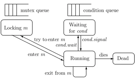
Entry procedures and procedures of a monitor can only access the local variables of the same monitor. These local variables cannot be accessed from outside the monitor. ! Remark 3. We assume that inside a monitor procedure a process is either (i) in the exe-cution state (i.e., running), or (ii) is in the waiting state (i.e., waiting) (see also Figure 11 below).
A process which has executed a cond.wait operation from inside a monitor procedure and has not yet resumed execution (see the following Remark 4), is not considered to be a process which executes that procedure. That process is on a waiting state and not in an execution state. Notice, however, when that waiting process starts the execution again, it will resume from the statement just after the cond.wait operation which made it to stop. Thus, it may be the case that while a process is waiting on a cond.wait operation on a procedure of a monitor, another process is executing the same or a distinct procedure of that same monitor.
We have the following properties.
(Mutual Exclusion) For each monitor at any given time, there exists at most one procedure of the monitor which is executed by a process, and that procedure, if it exists, is executed by exactly one process (This statement holds regardless whether it is relative to an entry procedure or a procedure).
(Process Locality) For each process at any given time, there exists at most one monitor procedure among the procedures of all monitors such that the process is either executing that procedure or waiting in that procedure (This statement holds regardless whether it is relative to an entry procedure or a procedure). ! Remark 4. A cond.wait operation performed on a condition variable cond, issued from inside a monitor procedure, causes the process which performs it, to be stopped and that process is made to wait for a future cond.signal operation to occur. This cond.signal operation will be performed by a different process. A cond.signal operation performed on