Alma Mater Studiorum · Università di Bologna
Scuola di Scienze
Corso di Laurea Magistrale in Fisica del Sistema Terra
Study of Jupiter’s auroral regions through the
measurements of the Juno/JIRAM instrument
Relatore:
Prof. Tiziano Maestri
Correlatori:
Dr. Bianca Maria Dinelli
-ISAC-CNR Bologna
Dr. Francesca Altieri
-IAPS-INAF Roma
Presentata da:
Chiara Castagnoli
Sessione II
Anno Accademico 2019/2020
Abstract
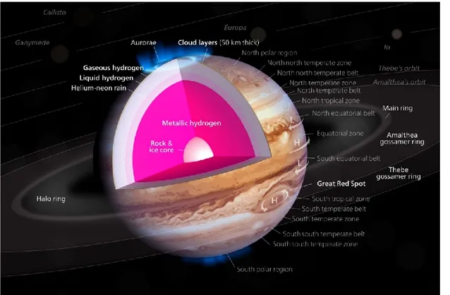
Lo strumento JIRAM (Jovian Auroral Infrared Mapper) a bordo della sonda spaziale Juno della NASA, in orbita attorno a Giove da luglio 2016, è stato progettato per eseguire il monitoraggio dell’atmosfera di Giove e delle sue aurore. Grazie all’orbita polare di Juno, i poli del pianeta sono stati osservati per la prima volta con una risoluzione spaziale molto più elevata di missioni spaziali precedenti. In questo lavoro di tesi, i dati di JIRAM, misurati nelle regioni polari, sono stati utilizzati per ricavare informazioni quantitative sulle specie CH4 e H3+ e sulla variabilità della loro distribuzione spaziale.
Gli spettri sono stati analizzati nella regione spettrale fra 3 𝜇m e 4 𝜇m, che è particolarmente favorevole per lo studio delle emissioni aurorali, a causa del quasi totale assorbimento della radiazione solare da parte degli strati più bassi dell’atmosfera Gioviana. A partire dai dati precedentemente analizzati per l’orbita JM0003 [Dinelli et al., Adriani et al. e Moriconi et al., 2017], il dataset è stato ampliato includendo osservazioni al di fuori degli ovali aurorali con un segnale più basso ed estendendo l’analisi ad orbite successive. Le prime orbite di Juno, dalla JM0003 alla JM0091, sono state esaminate per trovare quelle con una buona copertura delle zone polari da parte dello spettrometro e con un buon rapporto segnale rumore. Accanto all’orbita JM0003, sono state analizzate le orbite JM0071 e JM0081, risultate particolarmente promettenti per lo studio dell’aurora sud. Le misure spettroscopiche selezionate mostrano la presenza di emissioni di H3+ e CH4 sia nell’aurora sud
che nell’aurora nord e sono state analizzate usando una tecnica di inversione basata su un approccio di tipo bayesiano. Test preliminari hanno permesso di ottimizzare per il nuovo dataset il vettore di informazione a-priori e l’errore corrispondente. È stato inoltre possibile limitare i gradi di libertà dell’informazione alle sole abbondanze delle due specie emittenti e temperatura dell’H3+. Questo ha
permesso di evitare l’insorgere nelle quantità ricavate di bias causati dalla forte correlazione con le altre variabili di stato (temperatura di CH4 e alcuni parametri strumentali) e di diminuire i valori di
𝜒2. I risultati hanno confermato la presenza di una significativa concentrazione di metano in
prossimità di entrambi i poli, all’interno dell’ovale aurorale, e abbondanze confrontabili di H3+ nelle
due regioni aurorali, con valori generalmente compresi tra 2.0∙ 1012 cm−2e 2.8∙ 1012 cm−2 e alcuni
picchi superiori a 2.8∙ 1012 cm−2. Le temperature dell’H 3
+ risultano invece inferiori nell’aurora sud,
dove mediamente si osservano valori che non superano 825 K, mentre in corrispondenza dell’aurora nord le temperature si aggirano tra 800 K e 950 K. Il confronto di questi risultati con le immagini ricavate dalle osservazioni di JIRAM nella banda L ha inoltre consentito di studiare la morfologia delle aurore Gioviane e di evidenziare il dislocamento di alcuni gradi verso ovest dell’aurora sud nel periodo di tempo preso in esame.
Abstract
The Jovian Auroral Infrared Mapper (JIRAM) instrument aboard NASA’s Juno spacecraft, which has been orbiting Jupiter since July 2016, was designed to monitor the atmosphere of Jupiter and its aurorae. Due to Juno’s polar orbit, the poles of the planet have been observed with a much higher spatial resolution than previous space missions. In this thesis, JIRAM data measured over the polar regions, have been used to derive quantitative information on the species CH4and H3+ and on the
variability of their spatial distribution. JIRAM spectra have been analysed in the spectral region from 3 to 4 μm, that is particularly favourable for the study of the auroral emissions, due to the quasi-total absorption of the incoming solar radiation from the lowest layers of Jupiter atmosphere. Starting from the data previously analysed for the orbit JM0003 [Dinelli et al., Adriani et al. e Moriconi et al., 2017], the dataset has been enlarged to include observations outside the auroral ovals with a lower signal and extending the analysis to successive orbits. The first Juno orbits, from JM0003 to JM0091, have been examined in order to find the ones with both good polar coverage of the spectrometer measurements and good signal to noise ratio. Along with the JM0003, the orbits JM0071 and JM0081 have been analysed, resulting particularly promising for the study of the southern aurora. The selected spectroscopic measurements show the presence of H3+ and CH4emissions in both the southern aurora
and the northern aurora and have been analysed using an inversion technique based on a Bayesian approach. Preliminary tests have allowed to optimize for the new dataset the a-priori information vector and the corresponding error. It has also been possible to limit the degrees of freedom of the information to just the abundances of the two species and H3+ temperature. This has enabled to avoid
the retrieved quantities to be affected by biases produced by the strong correlation with the other state variables (CH4 temperature and some instrumental parameters) and to decrease the 𝜒2 values.
The results have confirmed the presence of a significant concentration of methane near both poles, within the auroral oval, and comparable abundances of H3+ in the two auroral regions, with values
generally ranging from 2.0∙ 1012 cm−2to 2.8∙ 1012 cm−2 e some peaks larger than 2.8∙ 1012 cm−2.
Instead, the H3+ temperatures appear lower in the south aurora, where on average the values do not
exceed 825 K, while in the northern aurora the temperatures span between 800 K and 950 K. The comparison of these results with the images obtained from the JIRAM’s observations in the L band has also allowed to study the morphology of the Jovian aurorae and to highlight the displacement of a few degrees westward of the south aurora over the time.
i
Contents
Introduction
... 1 1.Radiative transfer
... 3 1.1 Molecular spectroscopy ... 3 1.1.1 General principles ... 3 1.1.2 Molecular spectra ... 51.2 Absorption spectra of gaseous molecules ... 13
1.2.1 Spectral line shapes and absorption coefficient ... 14
1.2.2 Voigt profile... 16
1.3 Atmospheric Radiation ... 17
1.3.1 Electromagnetic radiation ... 17
1.3.2 Radiation Intensity and Flux ... 19
1.3.3 Black body radiation ... 21
1.3.4 Absorption, reflection, transmission coefficients and emissivity ... 23
1.3.5 Kirchhoff’s law ... 24
1.4 Radiative Transfer Theory ... 25
1.4.1 Radiative transfer equation: Schwarzschild’s equation ... 26
1.4.2 Schwarzschild’s equation general solution ... 27
1.4.3 Plane-parallel approximation ... 28
1.5 The Einstein coefficients ... 29
1.6 Remote Sensing ... 31
1.6.1 Brightness Temperature ... 32
2. Retrieval Methods
... 332.1.1 Introduction to the Inversion Problem ... 33
2.1.2 Bayes’ Theorem and Inversion Problem solution ... 35
2.1.3 Maximum likelihood method ... 36
2.1.4 Gauss-Newton method and Levenberg-Marquardt method ... 37
3. Jupiter
... 41ii
3.2 Introduction to Jupiter ... 46
3.2.1 Jupiter’s formation and migration ... 47
3.2.2 Jupiter’s orbit and rotation ... 48
3.3 Jupiter’s atmosphere ... 50
3.3.1 Composition of Jupiter’s atmosphere ... 50
3.3.2 Jupiter’s temperatures and vertical structure ... 51
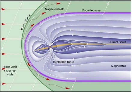
3.4 Jupiter’s magnetospheres ... 53
3.4.1 Planetary magnetospheres ... 53
3.4.2 Planetary plasmas: sources and dynamics ... 55
3.4.3 Structure of Jupiter’s magnetosphere ... 58
3.4.4 Jupiter’s plasma sources and dynamics ... 61
3.5 Jupiter’s Aurorae ... 62
3.5.1 Satellite footprints: Io footprint ... 63
3.5.2 Main Aurora ... 64
3.5.3 Polar Aurora ... 67
3.5.4 H3+ and its discovery on Jupiter ... 69
4. Detection of H
3+and CH
4on Jupiter by Juno/JIRAM
... 734.1 𝐇𝟑+ and 𝐂𝐇𝟒 detection in Jupiter’s auroral regions ... 73
4.1.1 H3+ emissions ... 73
4.1.2 CH4 emissions ... 74
4.2 Juno and JIRAM ... 75
4.2.1 Juno spacecraft and subsystem ... 75
4.2.2 JIRAM instrument ... 79
4.2.3 Planning strategy ... 83
4.2.4 Science observations ... 84
4.3 JIRAM Data ... 85
4.3.1 JIRAM observation modes ... 85
4.3.2 JIRAM Data Format ... 86
4.4 Major findings from JIRAM measurements ... 86
5. Analysis of H
3+and CH
4in Jupiter’s auroral regions
... 915.1 Data selection ... 91
5.5.1 Orbits selection ... 92
5.5.2 Spectra selection ... 96
iii
5.3 Retrieval Code ... 101
5.4 Initial guesses parameters ... 102
5.4.1 Determination of the CH4 effective temperature ... 103
5.4.2 Wavelength shift ... 106
5.5 Filtering of the retrievals ... 107
5.6 𝐇𝟑+ column density and temperature in Jupiter’s polar regions ... 112
5.6.1 H3+ column density and effective temperature maps for the North aurora ... 112
5.6.2 H3+ column density and effective temperature maps for the South aurora ... 115
5.7 𝐂𝐇𝟒 distribution in Jupiter’s polar regions ... 120
5.8 Aurorae’s morphology: comparison with the imager ... 124
5.8.1 H3+ column density and effective temperature maps for the North aurora ... 124
5.8.2 H3+ column density and effective temperature maps for the South aurora ... 125
Conclusions
... 129Bibliography
... 131iv Constants h = 6.62607015 ∙ 10−34 J∙s Planck constant 𝑘𝑏 = 1.380649 ∙ 10−23 J∙ K−1 Boltzmann constant 𝜎 = 5.67 ∙ 10−8 W∙ 𝑚−2∙ K−4 Stefan-Boltzmann constant c = 2.99792458 ∙ 108 𝑚 ∙ 𝑠−1 speed of light c2 = ℎ𝑐 𝑘⁄ = 1.43878 𝑒𝑟𝑔 𝑐𝑚 𝐾 Units of measurement
1
Introduction
Jupiter’s aurorae were first observed by the ultraviolet spectrometer (UVS) on board of Voyager 1 spacecraft in 1979. Successively, in the 1990’s, the Hubble Space Telescope collected several high-resolution images which showed bright emissions in Jupiter’s polar regions, similar to those occurring on Earth, but much more intense. Actually, Jupiter exhibits the most powerful auroras of the Solar System and, just as the Earth, these auroral emissions can be considered the projection of the magnetospheric processes, such as the precipitation of energetic particles along the planet’s magnetic field onto the upper atmosphere, where the collision with atmospheric gases causes the auroral phenomenon. After the discovery of the H3+ infrared spectrum by Oka (1980), and its detection in
Jupiter’s aurorae by Drossart et al. (1989), observations of the H3+ emissions have been used to study
the complex Jovian auroral morphology and the magnetospheric mechanisms leading to the aurorae’s occurrence. With this aim, the Jovian InfraRed Auroral Mapper (JIRAM) instrument, consisting in both an imager and a spectrometer has been developed and installed on board of the NASA Juno satellite. The imager of JIRAM acquires images in two spectral bands, M-band and L-band, where the L-band is dedicated to the auroral observations and allows detailed images of the H3+ distribution’s
morphology. The spectrometer measures the Jupiter spectrum in the spectral range from 2 µm to 5 µm over a slit featuring 256 pixels. This spectral range includes the infrared region from 3 to 4 µm, spectral range that is particularly suitable for mapping the H3+ thermal emissions, exploiting the
absorption by methane of most of the light coming and reflected from the lower atmosphere. Since trihydrogen cations form because of the ionization processes in the upper atmosphere, H3+ lines can
be detected thanks to the high contrast with respect to the dark background, enabling to map both H3+ concentration and temperature. During the first Juno’s orbit around Jupiter a large number of measurements have been collected in the auroral regions, showing both the emissions of H3+and of
CH4 in the 3-4 µm spectral range. Various analyses have then been performed on JIRAM’s first sequence of observations of Jupiter’s north and south poles. A first comparison of the UV and IR auroral features has revealed three main components of the aurorae’s morphology: the main oval, the polar emissions (poleward of the main oval) and the satellite footprints (equatorward of the main emission) [Gerard et al. (2017)]. With the help of a retrieval code developed to analyse JIRAM spectra, the H3+ effective temperatures and column densities along the line of sight (LOS) of each
observation have been retrieved. In particular, H3+ infrared emission lines have been used to derive
the atmospheric temperature, being the trihydrogen cations thermalized by the surrounding neutral atmosphere shortly after their formation, while the integrated column densities retrieved from the
2
emission lines’ intensity enabled the mapping of the ion distribution. Moreover, considering the detection of methane emissions in Jupiter’s aurorae, in the retrieval analysis the CH4 contribution to
the spectral signature has been taken into account; therefore, together with the H3+ data, methane
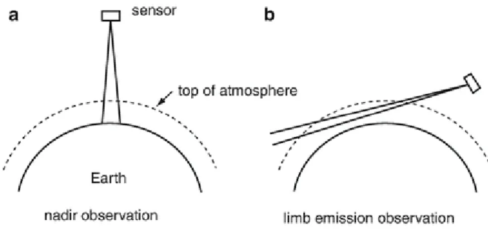
column density has been retrieved along the LOS [Dinelli et al. (2017); Adriani et al. (2017); Moriconi et al. (2017)]. In light of such results, this thesis is born with the purpose to integrate the work already done on JIRAM’s auroral observations acquired at nadir over Jupiter’s north and south pole during the first Juno’s orbit and to extend it to the subsequent orbits where JIRAM provided an optimal coverage of the auroral regions. In fact, initially the focus of this work has been posed on the first ten orbits of Juno satellite. However, only two of them have a sufficient coverage to study the Jovian northern aurora, whereas four orbits have been considered for the southern auroral emissions. Throughout all the examined orbits around the planet, the Juno/JIRAM instrument collected tens thousands of spectra, but only the most promising ones have been selected and analysed using the retrieval code described by Dinelli et al (2017) to determine temperatures and column densities of H3+ and CH4. The analysis’s outputs have been further filtered to reject those with higher 𝜒-test values and/or larger errors associated to the retrieved quantities and retain only the more reliable retrievals. Lastly, these ultimate results have been used to determine the morphological evolution of Jupiter’s aurorae over time, from one orbit to another, by comparing the resultant horizontal distributions of H3+ and CH
4temperatures and concentrations. Moreover, the final maps have been confronted with
the images from the imager, which differently from the spectrometer, cannot discern the two emitting species. All the procedures and methodologies adopted to draw the final conclusions are here presented in Chapter 5, preceded by four theoretical chapters having the purpose to provide the necessary background information for better understanding the target of this work and to introduce the JIRAM instrument.
- Chapter 1 consists in a general introduction to molecular spectroscopy and radiative transfer theory.
- Chapter 2 presents the Bayesian approach used for the inversion of JIRAM measurements. - Chapter 3 recalls the theory behind Jupiter and, in particular, describes the Jovian magnetosphere
and the auroral phenomena.
- Chapter 4 provides an overview of the physics that drives the Jovian aurorae and an accurate description of Juno/JIRAM instrument.
- Chapter 5 focuses on the data analysis performed in this thesis and on the discussion of the final results.
3
1. Radiative Transfer
1.1 Molecular spectroscopy
Spectroscopy is the science concerned with the investigation and measurement of spectra produced when materials interact with or emit electromagnetic (EM) radiation [van der Meer (2018)]. Based on the study of the EM radiation emitted, absorbed, or scattered by molecules, chemical information and molecular structure (bond lengths, angles, energy levels etc.) can be found.
1.1.1 General principles
A molecule is usually defined as a system of atoms, whose properties depend on ▪ the type of atoms constituting the molecule;
▪ the spatial structure of the molecule, i.e. the way in which the atoms are arranged, ▪ the binding energy of atoms or atomic groups,
The molecule stability results from a balance among the attractive and repulsive forces of the positively atomic nuclei (positively charged) and electrons (negatively charged). The molecule’s total energy resulting from these interacting forces can be sorted either as a potential energy or kinetic energy in 1. Translational energy: the kinetic energy of the molecules in a free environment due to their
motion.
2. Rotational energy: the kinetic energy associated with the rotational motion of the molecules. 3. Vibrational energy: the oscillatory motion of the atoms or groups of atoms within a molecule,
featuring a kinetic and potential energy exchange.
4. Electronic energy: energy stored as potential energy in excited electronic configurations. Thus,
𝐸𝑚𝑜𝑙 = 𝐸𝑡𝑟𝑎𝑛𝑠 + 𝐸 𝑖𝑛= 𝐸𝑡𝑟𝑎𝑛𝑠 + 𝐸𝑟𝑜𝑡+ 𝐸𝑣𝑖𝑏+ 𝐸𝑒𝑙 (1.1)
where 𝐸𝑚𝑜𝑙 is the total molecular energy given by the sum of translational energy and internal energies
(rotational, vibrational, and electronic). All these energies, except the translational one, are quantized: a quantum mechanical system (or particle) that is bond (i.e. spatially confined) can only assume certain discrete values, called energy levels. If a molecule (or atom) is at the lowest possible energy level, it and its electrons are said to be at the ground state, while if it is at a higher energy level, it is
4
said to be excited; also, if more than one quantum mechanical state is at the same energy, the energy level is said degenerate.
Fig 1.1 Molecular energy level diagram: (a) electronic transition, (b) vibrational transition, (c) rotational transition and
(d) roto-vibrational transition.
A molecular spectrum results when a molecule undergoes the absorption or emission of EM radiation jumping from a quantized energy state to another (Fig 1.1), however not all the transitions are allowed. In this regard, quantum mechanics laws define which pairs of energy levels can participate in energy exchange and the extent of the radiation absorbed or emitted. In first place, the condition for the absorption of EM radiation by a molecule going from a lower energy state, 𝐸′′, to a higher
one, 𝐸′, is that the frequency of the absorbed radiation must be related to the energy change, according
to the relation
𝐸′− 𝐸′′ = ℎ𝜈̃ = ℎ𝑐𝜈 (1.2)
where, ℎ𝜈 is the energy of the absorbed or emitted electromagnetic radiation, ℎ is the Plank’s constant, 𝜈 is the radiation frequency, 𝜈 = 𝜈̃ 𝑐⁄ is the radiation wavenumber, 𝐸′′ is the initial energy state and
𝐸′ the final energy state (see section 1.3.1). This phenomenon is referred to as stimulated absorption (Fig 1.2b). On the other hand, if a molecule in an excited energy state interact with an EM radiation of frequency 𝜈̃, and the transition to a lower energy state results in the emission of additional radiation
5
at the same frequency 𝜈̃, this is the case of stimulated emission (Fig 1.2c). Also, emission can happen spontaneously (spontaneous emission) (Fig 1.2a), without the presence of inducing radiation.
Fig 1.2 (a) spontaneous emission, (b) stimulated absorption and (c) stimulated emission.
According to what just said, the interaction of an electromagnetic radiation with the molecule can modify the incident wave, leaving a characteristic signature. For this interaction to take place, a force must act on the molecule in presence of an external magnetic field, and the existence of such a force does depend on the presence on the molecule of an electric or magnetic instantaneous dipole moment. In case of interactions through an electric dipole moment, the dipole moment 𝜇 ⃗⃗⃗ is directed from the negative to the positive charge and it is defined as
𝜇
⃗⃗⃗ = ∑ 𝑒𝑖𝑑 𝑖
𝑖
[Cm]
(1.3)
where 𝑒𝑖 are the electronic charges and 𝑑 𝑖 are the relative position vectors. The moment induced per
unit incident field is called polarizability of the molecule and it is related to the extent to which a molecule has a permanent dipole moment or can acquire an oscillating dipole moment through its vibrational motion.
1.1.2 Molecular spectra
The quantization of molecular energy levels and the resulting emission/absorption of radiation involving these levels depends on several mechanisms, as the interaction of the nuclei with each other and with the electrons. Thanks to their differences in magnitude, all these mechanisms, even if not clearly separated, can be examined independently by using a diatomic molecule model as an example.
6 Rotational energy levels
Molecules in gas phase are relatively far apart and free to rotate around their axis. Rotational energy depends on the moment of the inertia of the system, I: diatomic or linear triatomic molecules have two equal moments of inertia and two degrees of rotational freedom, while asymmetric top molecules have three unequal moments of inertia and three degrees of freedom (Fig 1.3, left).
Fig 1.3 (left) Axes of rotational freedom for linear diatomic, linear triatomic and asymmetric top molecules. (right) Rigid
rotor.
In quantum mechanics if a diatomic molecule is assumed to be rigid (internal vibrations are ignored), to predict its rotational energy a linear rigid rotor model can be used. The diatomic molecule is then considered to be a system of two-point masses, 𝑚1 and 𝑚2 located at fixed distances to their centre
of mass, with an internuclear distance 𝑟 (Fig 1.3, right). The moment of inertia is then estimated for each molecule as a function of the reduced mass 𝑚′ and the internuclear distance 𝑟. For a two-body
rigid rotator I is equal to
𝐼 = 𝑚1𝑟 + 𝑚2𝑟 = 𝑚′𝑟 (1.4)
where the reduce mass is defined as 𝑚′= 𝑚1𝑚2
𝑚1+𝑚2. Then, the kinetic energy of a rigid rotator is
𝐸𝑟𝑜𝑡 = 1 2 𝐼 𝜔
7
While for a classical rotator the angular velocity 𝜔, hence 𝐸𝑟𝑜𝑡, can assume any value, for a quantized
rotator quantum limitations occur, which result from a solution of the time-independent Schrödinger equation for reduced mass and null potential energy, i.e.
𝐼 𝜔 = ℎ
2𝜋 √𝐽 (𝐽 + 1) , 𝐽 = 0, 1, … (1.6) where J is the rotational quantum number. Consequently, the quantized rotational energy can be written
𝐸 𝑟𝑜𝑡 , 𝐽 =
ℎ2
8𝜋2𝐼𝐽(𝐽 + 1) = 𝐵ℎ𝑐𝐽(𝐽 + 1) (1.7)
with 𝐵 = ℎ
8𝜋2𝐼𝑐 , is called the rotational constant.
Molecular rotational spectra result when a molecule undergoes a transition from a rotational level to another. The allowed transitions are determined by quantum mechanics’ selection rules, which are defined in terms of allowed change in the quantum number characterizing the energy states. For a diatomic molecule, a transition between two rotational energy levels can occur when
1. the diatomic molecule has a permanent dipole moment; 2. the quantum condition ℎ𝜈̃ = 𝐸𝐽′− 𝐸𝐽′′ is satisfied;
3. the selection rule according to which only transitions among adjacent J-levels are allowed is met: ∆𝐽 = ±1.
According to these restrictions, the difference between two energy levels with lower and upper rotational quantum numbers 𝐽′and 𝐽′′respectively (𝐽′ = 𝐽′′+ 1 ) is
∆𝐹 =∆𝐸 ℎ𝑐 = 𝐵𝐽
′(𝐽′+ 1) − 𝐵𝐽′′(𝐽′′+ 1) = 2𝐵𝐽′= 𝜈
𝑟𝑜𝑡 (1.8)
where 𝜈𝑟𝑜𝑡 (cm−1) is the wavenumber of the spectral line resulting from the energy transition.
Vibrational energy levels
Real molecules are not rigid, as it is assumed when dealing with the rotational motion of a diatomic molecule: an aggregate of nuclear masses held together by elastic valence bonds can vibrate in one or more directions. In a diatomic molecule the two nuclei are in constant vibrational motion relative one
8
to another; therefore, it can be approximated to a two-masses vibrator with a natural harmonic frequency
𝜈̃ = 1 2𝜋(√
𝑘𝑒
𝑚′) (1.9)
where 𝑘𝑒 is the elastic force constant characteristic of the particular molecule. The resulting potential
energy of this system is
𝐸𝑝 = 2𝜋2 𝑚′ (𝑟 − 𝑟𝑒)2 𝜈̃2
(1.10)
where 𝑟𝑒 is the equilibrium distance. As it is shown in Fig 1.4, the potential energy of a classical
harmonic oscillator has a simple parabolic behaviour.
Fig 1.4 Potential energy of a harmonic and an anharmonic (Morse) two-masses vibrator (𝐷𝑒 is the binding energy for
rigid molecule, hence the dissociation energy, while 𝐷0 the true dissociation energy for non-rigid molecule due to the
zero point energy of the lowest vibrational level).
By the resolution of the one-dimensional time-independent Schrödinger equation, the eigenvalues defining the allowed vibrational energy levels can be found:
𝐸𝜈 = (𝜈 + 1 2) ℎ𝜈̃ = (𝜈 + 1 2) ℎ 2𝜋√ 𝑘𝑒 𝑚′ , 𝜈 = 0, 1, … (1.11)
9
Therefore, the conditions to observe a vibrational spectrum for a diatomic molecule are:
1. the change in the dipole moment of the molecule under vibration, which is not possible for a homonuclear diatomic molecule;
2. the quantum condition ℎ𝜈̃ = 𝐸𝜈′ − 𝐸𝜈′′ has to be satisfied, where 𝜈′ is any level (except
𝜈0) and 𝜈′′ is the lower level;
3. the selection rule according to which only transitions among adjacent 𝜈-levels are allowed is met: ∆𝜈 = ±1.
As a result, the difference between the two adjacent energy levels is equal to
𝛥𝐸𝜈 = ℎ 2𝜋√ 𝑘𝑒 𝑚′[(𝜈′+ 1 2) − (𝜈 ′′+1 2)] = ℎ𝜈̃ = ℎ𝑐 𝜈𝑣𝑖𝑏 (1.12)
where 𝜈𝑣𝑖𝑏 is the wavenumber of the transition (the absorption by a molecule cause the depletion of
the EM radiation of wavenumber 𝜈𝑣𝑖𝑏, resulting in a absorption spectral line). However, the harmonic
oscillator, hence the parabolic curve, well represents the potential energy of vibrating molecules for transition from 𝜈 = 0 to 𝜈 = 1, while for larger vibrational quantum number the repulsive forces make the curve steeper when the bond length is reduced and less steep when it is expanded. The result is an empirical function called Morse potential (Fig 1.4), which better represents the reality: the vibrational energy levels become increasingly dense with large quantum numbers and at certain value 𝜈, the molecule no longer vibrates but dissociates, because at larger distances the restoring force tends to zero (while the parabolic behaviour predicts an infinite increase of the potential energy with the increase of the internuclear distance).
Electronic energy levels
In a diatomic molecule the energy relations among nuclei and electros is more complex than for a single atom. In fact, electrons are not assigned to individual bonds between atoms, but are considered to move under the influence of the nuclei within the molecule. In order to describe the molecule’s electronic structure, the Molecular Orbital theory (MO) is used. This approach builds on the electron wave functions of quantum mechanics to describe chemical bonding. As a matter of fact, electrons may be considered either a particle or a wave: an electron in an atom may be described as occupying an atomic orbital, or by a wave function 𝛹 which is a solution of the Schrödinger equation. According
10
to this method, the electronic wave functions of the individual atoms constituting the molecules, called the atomic orbitals (AOs), are combined to obtain the wave function of the molecular orbitals.
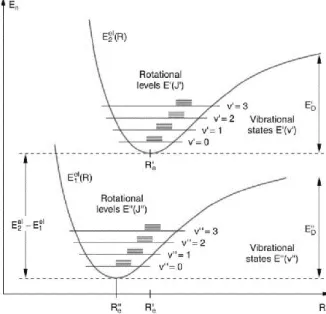
Fig 1.5 Rotational and vibrational levels in two different electronic states of a diatomic molecule.
The formation of molecular orbital occurs by the combination of atomic orbitals of proportional symmetry and comparable energy; therefore, the number of resulting molecular orbital is equal to the number of atomic orbitals, and while an atomic orbital is monocentric, a molecular orbital results to be polycentric. Consequently, molecular electronic spectra arise from the transition of an electron from a MO to another, where, since the diatomic molecule constantly undergoes vibrational motion, the potential energy of an electron in a particular MO is plotted relative to the internuclear separation in the molecule in a potential-energy diagram (Fig 1.5).
Roto-vibrational energy level
In real molecules the absolute separation of the different type of motions is rarely encountered. As it has already been mentioned, molecules without a permanent dipole moment can possess an oscillating dipole moment. A molecule in a given vibrational state can rotate, therefore each vibrational level is in reality divided into several rotational levels of energy equal to the sum of the vibrational and rotational energies. Being the difference among rotational energy levels of the order of 1-10 𝑐𝑚−1 ,
while the difference in the vibrational ones of the order of 1000 𝑐𝑚−1, the difference of magnitude
between the energy levels very often allows to separate the rotational levels belonging to one vibrational level to the ones belonging to another. Consequently, the more complex is the molecular
11
structure the higher is the number of the possible roto-vibrational transitions. For the simple case of absorption by a heteronuclear diatomic molecule with one degree of rotational freedom in the electronic ground state, the selection rules are 𝛥𝜈 = 1 and 𝛥𝐽 = ±1. Typically, at room temperature, only the ground vibrational state is populated 𝜈′′= 0, but several rotational states 𝐽 may be populated.
Therefore, the molecule can go to 𝜈′= 1, either to the next higher rotational level (𝛥𝐽 = +1), when
the energy of the rotational transition is added to the energy of the vibrational transition, increasing the transition energy gap, or, conversely, to the next lower one (𝛥𝐽 = −1), when the transition energy gap is decreased. Then, the total energy given by the sum of rotational and vibrational energy can be written 𝐸𝜈 = 𝐵ℎ𝑐 𝐽 (𝐽 + 1) + (𝜈 +1 2) ℎ 2𝜋 √ 𝑘𝑒 𝑚′ (1.13)
where the wavenumber of the corresponding absorption line is
𝜈 = ±2𝐵𝐽′+ 1 2𝜋𝑐√
𝑘𝑒
𝑚′ (1.14)
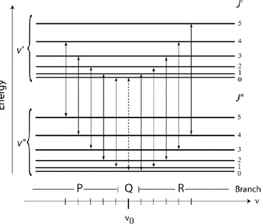
In a molecular roto-vibrational spectrum, the transition from one rotational level of the vibrational ground state to one rotational level in the vibrational excited state generates a spectral line and the assembly of the lines corresponding to a certain vibrational transition is called a vibrational band.
12
As shown in Fig 1.6, the vibrational transitions belonging to the same vibrational band can be separated in the following branches
1. P-branch → The transitions with selection rule 𝜟𝑱 = −𝟏 represented on the left of the central dotted vertical line. This group is the lower-energy, hence lower-frequency portion of the band.
2. R-branch → The transitions with selection rule 𝜟𝑱 = +𝟏, represented on the right of the central dotted vertical lines. This group is the higher-energy, hence higher-frequency portion of the band.
3. Q-branch → It is the part of the infrared spectrum involving vibrational transitions with the same rotational quantum number in ground and excited states (𝜟𝑱 = 𝟎). The position of the Q-branch is then defined by the term 𝜈0.
The roto-vibrational spectra are also classified according to the direction of the dipole moment change vector:
▪ P-branch and R-branch are called parallel branches because the dipole moment oscillates parallel to the internuclear axis. For this vibrational mode, the transition 𝛥𝐽 = 0 is forbidden, therefore no spectral line appears.
▪ Q-branch is called perpendicular branch because for perpendicular vibration the transition 𝛥𝐽 = 0 is allowed.
Fig 1.7 (left) Ideal roto-vibrational spectrum and (right) Real roto-vibrational spectrum.
Actually, the R-branch is not a perfect mirror of the P-branch, as it may appear from an ideal roto-vibrational spectrum (Fig 1.7, left). For real molecules, due to the increased moment of inertia in higher vibrational levels and the consequent reduction of rotational energy, the distance between
13
rotational levels in the higher vibrational energy level 𝜈′ is slightly smaller than in the 𝜈′′; moreover,
the frequency spacing between the spectral lines decreases with increasing frequency. Consequently, real roto-vibrational spectra show several asymmetric features (Fig 1.7, right).
Let now call 𝑓𝜈 = 𝑛𝑋,𝜈⁄𝑛𝑋 the population fraction of the excited level 𝜈 of a molecule X with
respect to the number density of the molecule. At thermal equilibrium1, 𝑓
𝜈 is given by the Boltzmann
factor, i.e.
𝑓𝜈 = 𝑔𝜈𝑒
−(𝑐2𝐸𝜈⁄𝑇)
𝑄𝑋(𝑇) (1.15)
where𝑔𝜈 is the degeneracy factor of level 𝜈, 𝑐2 is a constant and 𝑄𝑋(𝑇) is the partition sum of molecule X at temperature T, given by
𝑄𝑋(𝑇) = ∑ 𝑔𝜈𝑒−(𝑐2𝐸𝜈⁄𝑇) 𝜈
(1.16)
1.2 Absorption spectra of gaseous molecules
As already seen, molecular spectra are much more complicated than those of atoms and three types of absorption (or emission) spectra can be observed, with different absorption features, as the ones represented in Fig 1.8, left:
1. lines: sharp lines of finite width. 2. bands: aggregation of lines.
3. spectral continuum: atmospheric absorption which do not exhibit a line-like structure and it varies smoothly with the wavelength.
While within liquids and solids the absorption and emission take place throughout a continuum spectrum of wavenumbers, due to the strong interaction between molecules, gases produce line spectra.
1The thermodynamic equilibrium is the state of a physical system in which the quantities that specify its properties remain
14
1.2.1 Spectral line shapes and absorption coefficient
An absorption line is defined by three main factors: the central position of the line, such as the central wavenumber 𝜈0, the strength (or intensity, S) of the line and the shape factor (or line profile, f). The
condition for a strictly monochromatic absorption/emission to occur at 𝜈 and for the absorption line to appear like a Dirac 𝛿-function, is that the energy involved for each gaseous molecule must be 𝛥𝛦 = ℎ𝑐𝜈. However, in the atmosphere three processes may cause the broadening of spectral lines:
1. Natural broadening 2. Collision broadening 3. Doppler broadening
which are individually explained below and are represented in Fig 1.8, right.
Fig 1.8 (left)Types of absorption/emission spectra: (top) lines, (middle) bands and (bottom) spectral continuum. (right)
Comparison of normalized line broadening profiles, where ν is frequency and ∆ν is the Doppler width for the Doppler and Voight profiles and the Lorentz width for the Lorentz profile [Thomas (1999)].
1. Natural broadening
Every excited quantum state has finite duration, after which it spontaneously decays to the lower energy state. Due to their finite lifetime, energy levels are not infinitesimally narrow but have to be replaced by an energy distribution; therefore, the energy of a given state cannot be determined with infinitesimal precision. Heisenberg’s uncertainty principle connects the uncertainty 𝛥𝛦 of the
15
energy E of any atomic system with its mean lifetime 𝛥𝑡. If 𝛥𝛦 and 𝛥𝑡 are defined as the standard deviations of the respective distribution, the uncertainty principle demands
𝛥𝛦 ∙ 𝛥𝑡 ≈ ℎ
2𝜋 (1.17)
(h is the Planck constant). Consequently, a short lifetime will have a large energy uncertainty; hence,
∆𝜈 ≈∆𝐸 ℎ ≈
1
2𝜋 ∆𝑡 (1.18)
it will result in a broadening of the spectral line. The Michelson-Lorentz theory predicts the shape of this broadened line, which correspond to a Lorentzian line:
𝑘𝑁(𝜈) = 𝑆𝑓𝑁(𝜈) = 𝑆 𝜋 𝛼𝑁 (𝜈 − 𝜈0)2+ 𝛼 𝑁2 (1.19) where 𝑆 = ∫ 𝑘𝑁(𝜈) +∞
−∞ 𝑑𝜈 is the line strength and 𝛼𝑁 the line half width, which corresponds to
the distance from the centre of the line at half maximum power. The value of 𝛼𝑁 is independent
of wavelength and it is of the order of 10−5nm.
2. Collision broadening
This broadening results from the variation of the molecular potentials, and consequently of the energy levels, caused by inelastic and elastic collisions between a molecule and the surrounding ones occurring during emission/absorption processes. When the partial pressure of the absorbing gas constitutes only a small fraction of the total gas pressure, the Michelson-Lorentz theory used before can be exploited; therefore, this pressure broadening follows a Lorentz line shape:
𝑘𝐶(𝜈) = 𝑆𝑓𝐶(𝜈 − 𝜈0) =𝑆 𝜋
𝛼𝐶
(𝜈 − 𝜈0)2+ 𝛼𝐶2
(1.20)
where 𝛼𝐶 , which is several order of magnitude greater than 𝛼𝑁, is inversely proportional to the mean
free path, hence varies with pressure and temperature. Moreover, collisions between the same kind of particles produce a different broadening, called self-broadening, than the collisions with other molecules (i.e. occurring when we deal with a gas mixture), called the foreign-broadening that is evaluated as the average effect of the collisions between the separate gases.
16 3. Doppler broadening
Because in gas phase the molecules possess a Maxwell velocity distribution related to the temperature of the gas itself, in absence of collisions spectral lines exhibit a finite width. In fact, the components of the velocity along the direction of observation produce a Doppler effect, which shifts the apparent frequency of the emitted or absorbed radiance. Defining the probability to have a relative velocity u between the absorber and the observer (using the Maxwell law) 𝑝(𝑢) = √ 𝑚
2𝜋𝑘𝑇 𝑒𝑥𝑝 (− 𝑚𝑢2
2𝑘𝑇) and
the Doppler shift for 𝑢 𝑐⁄ << 1, 𝜈 − 𝜈0 = 𝜈0𝑢
𝑐 , the Doppler line shape results
𝑘𝐷(𝜈) = 𝑆𝑓𝐷(𝜈 − 𝜈0) = 𝑆 √𝜋𝛼𝐷
𝑒𝑥𝑝 [−(𝜈 − 𝜈0)
2
𝛼𝐷2 ] (1.21)
where the Doppler line half width is defined
𝛼𝐷 = 𝜈0
𝑐√2𝑘𝑇 𝑀⁄ 𝐴 (1.22)
𝑀𝐴 is the molar mass.
1.2.2 Voigt profile
Because collisions are proportional to pressure, the collisional broadening dominates in those region of the atmosphere where the pressure is large, and therefore the broadening due to pressure is larger than the one due to temperature (e.g. Earth’s troposphere); instead, the Doppler broadening is dominant where the molecules mean free path is large and the temperature broadening dominates (e.g. Earth’s upper stratosphere). However, there are region where neither of the two processes dominates, thus the final line shapes can be represented by a convolution of the two: the collision broadened shape is shifted by the Doppler effect and averaged over the Maxwell distribution. The resulting profile is called Voigt profile (Fig 1.8, right) and it is defined as
𝑓𝑉(𝜈 − 𝜈0 ) = ∫ 𝑓𝐶(𝜈′− 𝜈0) +∞ −∞ 𝑓𝐶(𝜈 − 𝜈′) 𝑑𝜈′= 𝛼𝐶 𝜋3 2⁄ 𝛼 𝐷 ∫ 1 (𝜈′− 𝜈 0)2+ 𝛼𝐶2 𝑒𝑥𝑝 [−(𝜈 − 𝜈 ′)2 𝛼𝐷2 ] +∞ −∞ (1.23)
17
1.3 Atmospheric Radiation
1.3.1 Electromagnetic radiation
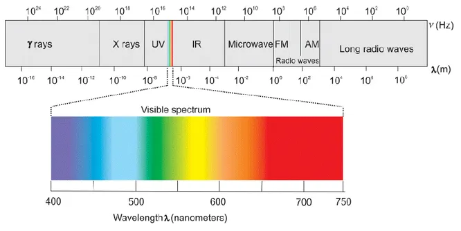
The electromagnetic radiation is an electric and magnetic disturbance traveling through space at the speed of light. The EM radiation has a dual nature, showing both wave and particulate properties. Electromagnetic waves can be classified in the electromagnetic spectrum (Fig 1.9) according to their wavelengths (𝜆) or frequency (𝜈̃), which are connected to each other by the relation:
𝜆 = 𝑐
𝜈̃ (1.24)
where c is the speed of light in vacuum.
Fig 1.9 Electromagnetic spectrum.
The EM radiation can be classified (in increasing order of wavelength) as: 1. Gamma radiation
A γ-ray is a penetrating form of electromagnetic radiation arising from the radioactive decay of atomic nuclei. It consists of the shortest wavelength electromagnetic waves (≤3· 10−13m) that
corresponds to the highest photon energy (≥100 keV). 2. X-radiation
An X-ray is a penetrating form of high-energy electromagnetic radiation. Generally, X-rays have a wavelength ranging from 10 pm to 10 nm and energies in the range 124 eV to 124 keV.
18 3. Ultraviolet radiation
UV radiation constitutes about 10% of the total electromagnetic radiation output from the Sun and consists in an electromagnetic radiation whose wavelength ranges from 10 nm to 400 nm. Together with X-rays and γ-rays, short wavelength UVs are called ionizing radiations, because they can cause chemical reactions to take place or many substances to glow.
4. Visible light
Visible light represents the region of the EM spectrum the human eye is most sensitive to. Typically, electromagnetic radiation with wavelengths between 380-760 nm, typically absorbed and emitted by electrons in molecules and atoms is perceived as visible light.
5. Infrared radiation
Infrared is that part of the electromagnetic spectrum characterized by wavelengths extending from the nominal red edge of the visible spectrum at 750 nm to 1 mm. Any object with a temperature emits infrared radiation (IR), also known as thermal radiation. The wavelength at which a body radiates most intensely depends on its temperature; therefore, the infrared range is often subdivided into three regions, which are used for observation of different temperature ranges, and hence different environments in space.
▪ Near-Infrared (NIR) [2500 -750 nm] → The physical processes that are relevant for this range are similar to those for visible light. Also, the highest frequencies in this region can be detected directly by many types of solid-state image sensors for infrared photography. ▪ Mid-Infrared (MIR) [10 -2.5 μm] → The mid-infrared spectral region contains strong
characteristic vibrational transitions of many important molecules, as well as two atmospheric transmission windows of 3-5 μm and 8-13 μm.
▪ Far-Infrared (FIR) [1mm -10 μm] → Radiation within this range are typically absorbed by rotational modes in gas-phase molecules, by molecular motions in liquids, and by phonons in solids. Due to the strong absorption by water within this range, Earth’s atmosphere appears opaque to FIR radiations; however, few wavelength ranges (“windows”) allow their partial transmission and can be used for astronomy.
19 6. Microwave radiation
MW radiation is a form of electromagnetic radiation with wavelengths ranging from about 1 m to 1 mm. Different from light and infrared radiations which are mostly absorbed by the surface, microwaves can penetrate into materials. Moreover, at the low end of this band the atmosphere is mainly transparent.
7. Radio waves
Radio waves have the longest wavelengths in the electromagnetic spectrum, exhibiting frequency between 30 hertz (Hz) and 300 gigahertz (GHz). Radio waves are widely used to transmit information across distances in radio communication system (mobile phone, satellites, etc.). In fact, Earth's atmosphere is mainly transparent to radio waves, except for layers of charged particles in the ionosphere which can reflect certain frequencies.
Conventionally, to describe the radiation emitted from the sun the wavelength in micrometers (µm) is used. In the case of infrared radiation, it is conventional to use the wavenumber 𝜈 (cm−1)
𝜈 =1 𝜆=
𝜈̃
𝑐 (1.25)
Finally, in the microwave region the frequency in gigahertz (GHz) is used.
Electromagnetic radiation can also be described as a stream of massless particles, called photons, having an energy
𝜀𝑝ℎ𝑜𝑡𝑜𝑛 = ℎ𝜈̃ = ℎ 𝑐
𝜆= ℎ𝑐𝜈 (1.26)
where h is the Plank’s constant.
1.3.2 Radiation Intensity and Flux
When radiative energy leaves a medium (e.g. a plane surface) end enters another, the resultant energy flux shows different strengths in different directions. Similarly, the EM radiation passing through any point inside any medium tends to be variable with the direction. Therefore, in order to quantify the intensity of the radiation in a certain direction it is necessary to introduce the concept of solid angle,
20
which is denoted with Ω and it is expressed in a dimensionless unit called steradian (sr). A solid angle is defined as the ratio between the area 𝜎 of a spherical surface intercepted at the core and the square of the radius, r
𝛺 = 𝜎
𝑟2 (1.27)
Therefore, it can be said that “the area of a surface on a sphere of unit radius is equivalent in magnitude to the solid angle it subtends”, resulting both equal to 4𝜋. A more relevant case to radiation emitted/received by a surface is that of the hemisphere, corresponding to a solid angle of 2𝜋.
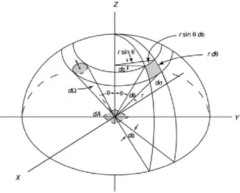
Let now consider a sphere with its central point in O and imagine a line starting from point O and intersecting a differential surface 𝑑𝜎 at distance r from the centre of the sphere. The resulting differential solid angle in polar coordinates (Fig 1.10) is
𝑑𝛺 = 𝑑𝜎
𝑟2 = 𝑠𝑖𝑛𝜃 𝑑𝜃 𝑑𝜙 (1.28)
where 𝜃 and 𝜙 are respectively the zenith angle, which is angle between the zenith (the point in the celestial sphere directly located on the observer’s ascending vertical) and the direction observed, and the azimuth angle, namely the angle of the object around the horizon, usually measured from true north and increasing eastward.
Fig 1.10 Differential solid angle in polar coordinates.
Once defined the solid angle, two concepts can be introduced: the radiation intensity (or Radiance) and the radiation flux (or Irradiance).
21
1. The monochromatic Radiance, 𝐿𝜆 → It is a directional quantity defined as the radiant energy
(𝑑𝐸𝜆) emitted, received, or transmitted by a surface (dA) per unit time (dt) per unit solid
angle (d𝛺) per unit area normal to the pencil of ray and per unit of wavelength (d𝜆) (or frequency, d𝜈̃), i.e.
𝐿𝜆 = 𝑑𝐸𝜆
𝑑𝑡 𝑑𝛺 𝑑𝐴 𝑐𝑜𝑠𝜃 𝑑𝜆 (1.29)
The SI unit for the radiance is [𝑊 𝑚−2 𝑠𝑟−1 µ𝑚−1].
2. The monochromatic Irradiance, 𝐹𝜆 → It is defined as the integral over the entire hemisphere of
the normal component of the radiance, i.e.
𝐹𝜆 = ∫ 𝐿𝜆 2𝜋 𝑐𝑜𝑠𝜃 𝑑𝛺 = ∫ ∫ 𝐿𝜆 𝑐𝑜𝑠𝜃 𝑠𝑖𝑛𝜃 𝜋 2 ⁄ 0 𝑑𝜃 𝑑𝜙 2𝜋 0 (1.30)
where this relation in case of an isotropic radiation (the intensity of the radiation is independent of the direction) results
𝐹𝜆 = 𝜋𝐿𝜆 (1.31)
The SI unit for the monochromatic Irradiance is then [𝑊 𝑚−2 µ𝑚−1].
3. The total Irradiance, F → It is the flux density (energy per area per time) for all the wavelengths, obtained by integrating the monochromatic irradiance over the entire electromagnetic spectrum, i.e.
𝐹 = ∫ 𝐹𝜆
∞ 0
𝑑𝜆 (1.32)
whit SI unit [𝑊 𝑚−2]. Similarly, the total Radiance L, can be obtained with unit [𝑊 𝑚−2 𝑠𝑟−1].
1.3.3 Black body radiation
According to the third law of thermodynamics, all the matter at a temperature above the absolute zero emits energy in form of EM radiation, in all the directions and over a wide range of wavelengths. The studies of the radiation are based on an ideal body, the black body, which is a perfect emitter and absorber: it shows the maximum possible emission at all wavelengths and absorbs all the incident
22
radiation. The black body radiance can be expressed as a function of 𝜆, 𝜈̃ or 𝜈, in unit of energy/area/time/sr/wavelength, frequency, or wavenumber, using the Plank’s law represented by these three relations 𝐵𝜆(𝑇) =2ℎ𝑐 2 𝜆5 1 𝑒ℎ𝑐⁄𝜆𝑘𝑏𝑇 − 1 𝐵𝜈̃(𝑇) =2ℎ 𝑐2 𝜈̃3 𝑒ℎ𝜈̃⁄𝑘𝑏𝑇 − 1 𝐵𝜈(𝑇) = 2ℎ𝑐2 𝜈 3 𝑒ℎ𝑐𝜈⁄𝑘𝑏𝑇 − 1 (1.33)
where 𝑘𝑏 is the Boltzmann constant and T the absolute temperature of the body. The resulting
distribution of black body radiance as a function of the wavelength is shown in Fig 1.11. The black body curve also exhibits an interesting behaviour: the maximum of intensity shifts to shorter wavelengths as the temperature increases, following the well know Wien’s law
𝜆𝑚𝑎𝑥 = 2898
𝑇 (𝜇𝑚) (1.34)
Fig 1.11 Spectral intensity distribution of Plank’s back body radiation as a function of wavelength for different
23
Another important law is the Stefan-Boltzmann law, which can be obtained from the Plank’s law, by firstly deriving the spectral irradiance of a black body exiting a plane surface
𝐹𝜆(𝑇) = ∫ 𝐵𝜆(𝑇)𝑐𝑜𝑠𝜃𝑑Ω = 𝜋𝐵𝜆(𝑇) 2𝜋
(1.35)
then, integrating it over the entire spectrum
𝐹𝜆(𝑇) = ∫ 𝜋𝐵𝜆(𝑇)𝑑𝜆 = 𝜎𝑇4 ∞
0
(1.36)
where 𝜎 is the Stefan-Boltzmann constant.
1.3.4 Absorption, reflection, transmission coefficients and emissivity
As already mentioned before, the temperatures of all objects are higher than the absolute zero, therefore they all are able to emit radiation. The definition of emissivity exploits the idea of the black body. As a matter of fact, the emissivity (𝜀) of a surface represents the ratio of the radiation emitted by the surface at a particular temperature to that emitted by a black body at the same temperature, and assumes values between 0 and 1. Therefore, the emissivity can be seen as a measure of how closely a surface approximate a black body, whose emissivity is equal to the unit. The emissivity varies not only with the surface’s temperature, but also with the wavelength and the direction of the emitted radiation, hence it can be expressed as a spectral directional emissivity and defined as the ratio of the intensity of the radiation emitted by the surface at a specific wavelength in a certain direction to the intensity of radiation emitted by a black body at the same temperature and wavelength.
𝜀𝜆(𝜃, 𝜙, 𝑇) =𝐿𝜆(𝜃, 𝜙, 𝑇)
𝐵𝜆(𝜆, 𝑇) (1.37)
A more generic definition is that of total hemispherical emissivity, representing the ratio of the total radiation energy emitted by the surface to that of a black body of the same surface area at the same temperature, i.e.
𝜀(𝑇) = 𝐿(𝑇)
24
Because bodies emit constantly, they are also bombarded by radiations coming from all the direction and at different wavelengths. When a radiation with a particular wavelength impacts a surface, part of it can be absorbed, part reflected, and part transmitted by the medium. In particular, the fraction of irradiation absorbed is called absorptivity, 𝛼𝜆, the fraction reflected by the surface is called reflectivity,
𝜌𝜆, and the fraction transmitted is the transmissivity, 𝜏𝜆, that are given by the ratio of the radiation energy incident on the surface with the portion of irradiation absorbed, reflected and transmitted, respectively. All these quantities have a value between 0 and 1, therefore the conservation of energy implies 𝛼𝜆 + 𝜌𝜆+ 𝜏𝜆 = 1 (1.39) where, • black body, 𝛼𝜆=1, 𝜌𝜆=0, 𝜏𝜆=0 • perfect window, 𝜏𝜆=1, 𝛼𝜆=1, 𝜌𝜆=0 • opaque surface, 𝜏𝜆=0, 𝛼𝜆 + 𝜌𝜆 = 1
It has to be noted that the absorptivity of a material is almost independent from the surface temperature: while the energy absorbed by a body depends on the incident electromagnetic radiation and on the absorptivity of the medium, the energy emitted depends on both emissivity and temperature.
1.3.5 Kirchhoff’s law
The relation between the emission and the absorption of a real surface is described by the Kirchhoff’s law. In order to introduce this law, let consider an object in a cavity whose interior walls radiate as a black body. Suppose, then, that the object and the walls are in radiative equilibrium, i.e. for the second law of thermodynamics they are at the same temperature. When a radiation arrives to the object at a certain wavelength and from a particular direction, the body absorbs a fraction 𝛼𝜆 of the incident
radiation. Therefore, to conserve the radiative equilibrium the body must return the same monochromatic intensity at each wavelength and along each path. Remembering that the object and the walls of the cavity are at the same temperature, it follows that at all wavelength its emissivity must be equal to its absorptivity. This result is at the base of the Kirchhoff law, which states that a medium
25
in thermodynamic equilibrium with its environment can absorb radiation of a certain wavelength and at the same time emit radiation of that wavelength. Consequently, the emissivity of the medium at that wavelength, 𝜀𝜆, is equal to its absorptivity at the same wavelength, 𝛼𝜆:
𝜀𝜆 = 𝛼𝜆 (1.40)
As underlined before, this relation requires the condition of thermodynamic equilibrium, which represents an ideal case, quite far from the real state of planetary atmospheres. However, in a localized volume, the atmosphere can be considered approximately isotropic and with a uniform temperature, where energy transitions are governed by molecular collisions. In this condition, called local thermodynamic equilibrium or LTE, the intrinsic properties of the atmosphere do vary in space and time, but much more slowly than the phenomenon under study; therefore, for any point one can assume the thermodynamic equilibrium conditions to be valid in some neighbourhood of that point. Consequently, the Planck function (which is derived under thermodynamic equilibrium conditions) can be used to represent the spectral radiance emitted by a given atmospheric layer and the Kirchhoff law can be applied.
1.2 Radiative Transfer theory
In order to introduce the equation of radiative transfer, let study extinction and emission processes. During an absorption process the radiative energy is turned into internal or kinetic energy, emission transforms internal or kinetic energy into radiative energy, whereas scattering involves the transfer of radiative to internal to radiative energy; therefore, the intensity of the radiation decreases when an extinction occurs and increases during emission. Let’s consider extinction due to absorption of a beam passing through a thin atmospheric layer, ds, along a specific path. For each particle that the beam encounters, its monochromatic intensity is decreased by the increment
26
where 𝜌𝑎 represents the mass density, while 𝑘𝑎𝜆 is defined as the mass absorption cross section [𝑚2⁄𝑘𝑔],
which depends on the pressure, the temperature and on the spectral features of the absorber (from now on the notation underlying the spectral dependence of 𝑘𝑎 and L will be omitted for simplicity).
This formula is referred to as the Beer-Bouguer-Lambert’s law.
1.4.1 Radiative Transfer equation: Schwarzschild’s equation
In order to determine the fraction of incident beam (or pencil of radiation) attenuated due to absorption, the previous equation may be integrated between 0 and d, thus
𝐿(𝑑) = 𝐿(0)𝑒− ∫ 𝑘0𝑑 𝑎𝜌𝑎𝑑𝑠 (1.42)
This formula introduces the definition of path’s transmissivity
𝑇𝑟 = 𝑒− ∫ 𝑘0𝑑 𝑎𝜌𝑎𝑑𝑠 (1.43)
where the exponential is a dimensionless number, called optical depth and denoted by 𝜏, giving an estimate of how opaque a medium is to radiation passing through it. Assuming, then, to measure the attenuation from the top of the atmosphere (TOA, z=∞) downward in the nadir direction, the relation becomes
𝐿 = 𝐿0 𝑒−𝜏 (1.44)
where 𝐿0 represents the radiance at z=0. Based on the energy conservation discussed in section [1.3.4],
in a non-scattering atmosphere the relation between absorption and transmission in an atmospheric layer of thickness 𝛥𝑧 is given by
𝛼(𝛥𝑧) = 1 − 𝑇𝑟 (1.45)
and assuming the atmospheric slab to be very thin, the transmissivity results 𝑇𝑟 ≅ 1 − 𝑘𝑎 𝜌𝑎 Δ𝑧,
hence 𝛼 = 𝜏. From here, suppose that the atmosphere is in LTE conditions, thus the Kirchhoff’s law can be used to determine the radiation emitted per unit area by the atmospheric slab, i.e.
27
𝜀𝐵(𝑇) = 𝑘𝑎𝜌𝑎𝛥𝑧𝐵(𝑇) (1.46)
The radiative transfer equation is then obtained by combining the absorption and emission processes, leading to the Schwarzschild’s equation in a differential form:
𝑑𝐿 = −𝐿 𝑘𝑎𝜌𝑎𝑑𝑧 + 𝐵𝑎𝑘𝑎𝜌𝑎𝑑𝑧 (1.47) Considering 𝑑𝜏(𝑧) = −𝑘𝑎 𝜌𝑎𝑑𝑧, the RT equation can also be written as
𝑑𝐿
𝑑𝜏 = 𝐿 − 𝐵 (1.48)
which may be solved to give both the upward (or upwelling, 𝐿↑) and downward (or downwelling,
𝐿↓) intensities.
1.4.2 Schwarzschild’s equation general solution
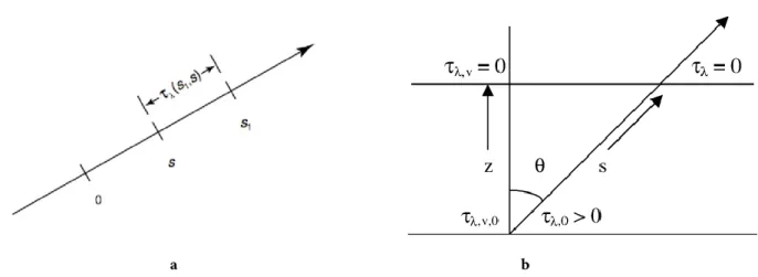
The equation RT equation found in the previous section can be solved by defining the monochromatic optical depth of a medium between two points 𝑠 and 𝑠1 (Fig 1.12a) as
𝜏(𝑠1, 𝑠) = ∫ 𝑘𝜌𝑑𝑠′
𝑠1
𝑠
(1.49)
Therefore, the differential form of the RT equation becomes
− 𝑑𝐿(𝑠)
𝑑𝜏(𝑠1, 𝑠)= −𝐿(𝑠) + 𝐵[𝑇(𝑠)] (1.50) By multiplying this result for 𝑒−𝜏(𝑠1,𝑠)∙ 𝑑𝜏(𝑠
1, 𝑠) and by integrating the thickness from 0 to 𝑠1, the
general solution of the Schwarzschild’s equation results
𝐿(𝑠1) = 𝐿(0) 𝑒−𝜏(𝑠1,0)+ ∫ 𝐵[𝑇(𝑠)] 𝑠1
0
28
where the first term in the right-hand side of the equation represents the attenuation of the radiation intensity due to absorption by the medium, while the second term is associated to the medium’s emission along the path from 0 to 𝑠1.
a b
Fig 1.12 (a) Schematic representation of the optical thickness of a medium between two point 𝑠 and 𝑠1. (b) Optical
depth along a ray path in a plane parallel atmosphere [Sánchez-Bajo et al, 2002].
1.4.3 Plane-parallel approximation
To facilitates many radiative transfer calculations and deal with a complex atmospheric vertical structure, a plane-parallel model, as the one shown in Fig 1.12b, can be used. This approximation consists in a set of atmospheric layers characterized by homogeneous properties; therefore, temperature and densities of the various component is assumed to vary with the high (or pressure) only. Traditionally, the vertical coordinate z is used to measure linear distances:
𝑧 = 𝑠 ∙ 𝑐𝑜𝑠𝜃 = 𝑠 ∙ 𝜇 → 𝑑𝑠 = 𝑑𝑧 𝑐𝑜𝑠𝜃 =
𝑑𝑧
𝜇 (1.52)
where 𝜃 is the zenith angle. With this approximation the flux density, passing through a certain atmospheric level either up- (↑, 𝜇 > 0) or downward (↓, 𝜇 < 0), is given by
𝐹↑↓(𝜏) = ∫ 𝐿↑↓(𝜏, 𝑐𝑜𝑠𝜃) 𝑐𝑜𝑠𝜃 𝑑𝛺 2𝜋 = 2𝜋 ∫ 𝐿↑↓(𝜏, 𝜇) 𝜇𝑑𝜇 1 0 (1.53)
29
The flux transmissivity of a layer can be approximated to the intensity transmissivity of parallel beam radiation passing through it with an average (or effective) zenith angle of 𝜃 = 53°
𝑇𝑟𝑓 = 2 ∫ 𝑒−𝜏 𝜇⁄ 1 0
𝜇𝑑𝜇 ≅ 𝑒−𝜏 𝜇̅⁄ (1.54)
where 1 𝜇̅⁄ ≡ 𝑠𝑒𝑐 53° = 1.66, is the diffusivity factor. Consequently,
𝐹↑↓(𝜏) = 𝜋𝐿↑↓(𝜏, 𝜇̅) (1.55)
Conventionally, the optical depth 𝜏 is measured downward from the top of the atmosphere (𝜏𝑡𝑜𝑝 = 0
and it increases for z decreasing) along the vertical optical path 𝑑𝑧 and it is defined as a measure of the light path in unit of the mean free path of photons (𝑙 = 1 𝑘𝜌)⁄ . In fact, when
• 𝜏 = 1 the intensity of the beam falls by 1/𝑒 over one mean free path • 𝜏 ≪ 1 the medium is said to be transparent or optically thin
• 𝜏 ≫ 1 the medium is said to be opaque or optically thick
1.5 The Einstein coefficients
Kirchhoff’s law, described in section 1.3.5, implies a relationship between emission and absorption at a microscopic level. This relation was first discovered by Einstein, who studied the properties of the single radiative transitions that couple matter with radiation. Let consider an ensemble of molecule X and the simple case of two discrete energy levels (Fig 1.13): the first of energy 𝐸, with a statistical weight 𝑔1 and the other of energy 𝐸 + ℎ𝜈0 and a statistical weight 𝑔2. As already seen in section
1.1.1, the radiative transition between this two levels are governed by three processes, which are here resumed to introduce the Einstein coefficients.
30 1. Spontaneous emission
This transition occurs when the system is in level 2 and drops to level 1 emitting a photon, and it occurs even in absence of a radiation field. In this case the Einstein A-coefficient, 𝑨𝟐𝟏,
is defined as the transition probability per unit time for spontaneous emission [𝑠−1].
2. Absorption
This occurs when the system makes a transition 1→2 by absorbing a photon of energy ℎ𝜈0.
Since there is no self-interaction of the radiation field, the probability per unit time of this process is proportional to the density of photons (or the mean intensity) at frequency 𝜈̃0,
namely where the line profile function 𝜙(𝜈̃) peaks. Therefore, the transition probability
per unit time of absorption is defined as 𝑩𝟏𝟐· 𝑱̅, where 𝐽̅ [erg cm−2 s−1 cm ]is the local
mean radiance at the transition energy ℎ𝜈0, while 𝐵12 [cm3erg−1cm−2] is the Einstein
B-coefficient.
3. Stimulated emission
Simulated emission is proportional to 𝐽̅ and causes the emission of a photon. Therefore, the
transition probability per unit time for simulated emission is defined as 𝑩𝟐𝟏· 𝑱̅, where 𝐵12
[cm3erg−1cm−2] is another Einstein B-coefficient.
The relation between these three coefficients can be obtained using a statistical approach first proposed by Einstein. Let consider an ensemble of molecules at equilibrium at temperature T with radiation. In thermodynamic equilibrium (TE) the number of transitions per unit time per unit volume out of state 1 is equal to the number of transition per unit time per unit volume into state 1. Therefore, defining 𝑛1 and 𝑛2 as the number densities of atoms in level 1 and 2, respectively, this
reduces to
𝑛1𝐵12𝐽̅ = 𝑛2𝐴21+ 𝑛2𝐵21𝐽̅ (1.56) where in TE the Boltzmann expression [see section 1.1.2, formula (1.15)] for the levels’ population ratios is 𝑛1 𝑛2 = 𝑔1𝑒 (−𝐸 𝑘⁄ 𝑏𝑇) 𝑔2𝑒[−(𝐸+ℎ𝜈0) 𝑘⁄ 𝑏𝑇] = 𝑔1 𝑔2 𝑒(ℎ𝜈0⁄𝑘𝑏𝑇) (1.57)
31
Therefore, combining (1.56) with (1.57), and solving for 𝐽̅
𝐽̅ = 𝐴21⁄𝐵21
(𝑛1⁄𝑛2)(𝐵12⁄𝐵21) − 1=
𝐴21⁄𝐵21
(𝑔1𝐵12⁄𝑔2𝐵21)𝑒(ℎ𝜈0⁄𝑘𝑏𝑇)− 1
(1.58)
and expressing the mean radiance with the Plank function at temperature T, the Einstein relations result: 𝑔1𝐵12= 𝑔2𝐵21 𝐴21= 2ℎ𝜈 3 𝑐2 𝐵21 (1.59)
These relations reflect the radiative properties 𝐴21, 𝐵12 and 𝐵21 of a single molecule and, different
from the Kirchhoff’s law, do not refer to the temperature T; therefore, even though they have been obtained in an equilibrium configuration, must hold whether or not the atoms are in thermodynamic equilibrium and can be considered an extension of the Kirchhoff’s law to include the nonthermal emission when the matter is not at TE.
1.6 Remote Sensing
Remote sensing is based on the interpretation of the radiometric measurements of the EM radiation in specific spectral intervals, which are sensitive to some physical property of the medium. Therefore, Remote Sensing can be defined as the science to obtain information on a target (object, area, or phenomenon) from distance, by sensor mounted on platforms (e.g. satellites) that use the entire electromagnetic spectrum. Remote sensing instruments can be classified into two categories: active or passive. An active sensor generates its own signal, which is successively measured when reflected, refracted, or scattered by a planetary surface or its atmosphere. A passive sensor is designed to receive, and measure either the natural emissions produced by constituents of the surface or atmosphere of a planet or the radiation emitted by an external source (typically the Sun or a star) and absorbed by the atmosphere.
32
1.6.1 Brightness Temperature
Many objects do not emit like black body; however, any measured spectral radiance can be represented as the radiation that a blackbody at a given temperature will emit. Moreover, applying the inverse of the Plank function to the measured radiation, a descriptive measure of the radiation in terms of temperature can be obtain:
𝑇𝑏= ℎ𝑓 𝑘𝑏𝑙𝑛 (1 −2ℎ𝑓3 𝑐2𝐿 𝑓) (1.60)
This formula represents the Brightness Temperature 𝑇𝑏 (for a radiance at a given frequency) and it is
defined as the temperature of a black body that radiates the same surface brightness at a given frequency. This temperature can be either independent of, or highly dependent on the radiation’s wavelength, depending on the nature of the source and any subsequent absorption.

![Fig 3.3 Juno’s orbital grid. [NASA/JPL/Caltech]](https://thumb-eu.123doks.com/thumbv2/123dokorg/7383638.96701/52.892.127.768.578.781/fig-juno-s-orbital-grid-nasa-jpl-caltech.webp)