Automatic generation of synthetic datasets for digital pathology image analysis

Alma Mater Studiorum · University of Bologna

School of Science

Department of Physics and Astronomy Master Degree in Physics

Automatic Generation of Synthetic

Datasets for Digital Pathology Image

Analysis

Supervisor:

Dr. Enrico Giampieri

Co-supervisor:

Dr. Nico Curti

Submitted by:

Alessandro d’Agostino

Abstract

The project is inspired by an actual problem of timing and accessibility in the anal-ysis of histological samples in the health-care system. In this project, I address the problem of synthetic histological image generation for the purpose of training Neural Networks for the segmentation of real histological images. The collection of real histo-logical human-labeled samples is a very time consuming and expensive process and often is not representative of healthy samples, for the intrinsic nature of the medical analysis. The method I propose is based on the replication of the traditional specimen preparation technique in a virtual environment. The first step is the creation of a 3D virtual model of a region of the target human tissue. The model should represent all the key features of the tissue, and the richer it is the better will be the yielded result. The second step is to perform a sampling of the model through a virtual tomography process, which produces a first completely labeled image of the section. This image is then processed with different tools to achieve a histological-like aspect. The most significant aesthetical post-processing is given by the action of a style transfer neural network that transfers the typical histological visual texture on the synthetic image. This procedure is presented in detail for two specific models: one of pancreatic tissue and one of dermal tissue. The two resulting images compose a pair of images suitable for a supervised learning technique. The generation process is completely automatized and does not require the intervention of any human operator, hence it can be used to produce arbitrary large datasets. The synthetic images are inevitably less complex than the real samples and they offer an easier segmentation task to solve for the NN. However, the synthetic images are very abundant, and the training of a NN can take advantage of this feature, following the so-called curriculum learning strategy.

Table of Contents

Introduction 6

1 Theoretical Background 12

1.1 Histological Images Digitalization . . . 12

1.1.1 Slides Preparation for Optic Microscopic Observation . . . 15

1.1.2 Pancreas Microanatomy and Evidences of Neoplasms . . . 16

1.1.3 Skin Microanatomy and Evidences of Neoplasms . . . 18

1.2 Introduction to Deep Learning . . . 20

1.2.1 Perceptrons and Multilayer Feedforward Architecture . . . 20

1.2.2 Training Strategies in Deep Learning . . . 22

1.2.3 Training Algorithms - Error Back-Propagation . . . 24

1.3 Deep Learning-Based Segmentation Algorithms . . . 28

1.3.1 State of the Art on Deep Learning Segmentation . . . 29

1.3.2 Image Segmentation Datasets . . . 34

2 Technical Tools for Model Development 37 2.1 Quaternions . . . 37

2.2 Parametric L-Systems . . . 39

2.3 Voronoi Tassellation . . . 41

2.4 Saltelli Algorithm - Randon Number Generation . . . 43

2.5 Planar Section of a Polyhedron . . . 45

2.6 Perlin Noise . . . 47

2.7 Style-Transfer Neural Network . . . 49

2.8 Working Environment . . . 52

3 Tissue Models Development 53 3.1 Pancreatic Tissue Model . . . 53

3.1.1 2D Ramification . . . 53

3.1.2 Expansion to 3D . . . 55

3.1.3 Subdivision in Cells . . . 56

3.1.4 Cells Identity Assignment . . . 59

3.2 Dermal Tissue Model . . . 60

3.3 Synthetic Images Production . . . 63

3.3.1 Sectioning Process . . . 63

3.3.2 Aesthetical Post-processing . . . 65

Conclusions 72

Introduction

In the last decades, the development of Machine Learning (ML) and Deep Learning (DL) techniques has contaminated every aspect of the scientific world, with interesting results in many different research fields. The biomedical field is no exception to this and a lot of promising applications are taking form, especially as Computer-Aided Detection (CAD) systems which are tools to support for physicians during the diagnostic process. Medical doctors and the healthcare system in general collect a huge amount of data from patients during all the treatment, screening, and analysis activities in many different shapes, from anagraphical data to blood analysis to clinical images.

In fact in medicine, the study of images is ubiquitous and countless diagnostic proce-dures rely on it, such as X-ray imaging (CAT), nuclear imaging (SPECT, PET), magnetic resonance, and visual inspection of histological specimens after biopsies. The branch of artificial intelligence in the biomedical field that handles image analysis to assist physi-cians in their clinical decisions goes under the name of Digital Pathology Image Analysis (DPIA). In this thesis work, I want to focus on a specific application of DPIA in the histological images analysis field, with particular attention to some of the issues in the development of DL models able to handle these procedure.

Nowadays the great majority of analysis of histological specimens occurs through visual inspection, carried out by highly qualified experts. Some analysis, as cancer de-tection, requires the ability to distinguish if a region of tissue is healthy or not with high precision in very wide specimens. It is necessary to recognize structures and features of the image on different scales, like the state of the single cell’s nucleus to the arrang-ment or macrostructures in the specimens. The required level of detail is very high and the analysis are performed on images of very high resolution. This kind of procedure is typically very complex and requires prolonged times of analysis besides substantial economic efforts. Furthermore, the designated personnel for this type of analysis is often limited, leading to delicate issues of priority assignment while scheduling analysis, based on the estimated patient’s preliminary prognosis development. Some sort of support to this procedure could therefore lead to improvments to the analysis framework.

The problem of recognizing regions with different features within an image and de-tect their borders is known in computer vision as the segmentation task, and it’s quite widespread with countless different applications. In ML the segmentation problem is

Figure 1: Interleaving of tumor (green annotation) and non-tumor (yellow annotation) regions [29].

usually classified as a supervised task, because the algorithm in order to be trained properly requires an appropriate quantity of pre-labeled images, from which learn the rules through which distinguish different regions. This means that the development of segmentation algorithms for a specific application, as would be the one on histological images, would require a lot of starting material, previously analyzed from the same qual-ified expert responsible for the visual inspection mentioned before. A human operator is thus required to manually draw the boundaries, for example, between healthy and tumoral regions within a sample of tissue and to label them with their identity, as shown in Figure 1. The more the algorithm to train is complex the more starting material is required to adjust the model’s parameters and reach the desired efficacy.

The latest developed segmentation algorithms are based on DL techniques, hence based on the implementation of Neural Networks (NN) which process the input images and produce the corresponding segmentation. These models are typically very complex, with millions of parameters to adjust and tune, therefore they need a huge amount of pre-labeled images to learn their segmentation rules. This need for data is exactly the main focus of my thesis work. The shortage of ground truth images is indeed one of the toughest hurdles to overcome during the development of DL-based algorithms. Another important aspect to bear in mind is the quality of the ground truth material. It’s impossible for humans to label boundaries of different regions with pixel-perfect precision, while for machines the more precise is the input the more effective is the resulting algorithm.

are mainly based on the generation of synthetic labeled data to use during the train-ing phase. Some techniques achieve data augmentation manipulattrain-ing already available images and then generating new images, but as we will see this approach suffers from different issues. Here, I want to make an overview of some other interesting works on the generation of synthetic histological images, which have followed completely different paths and strategies from mine.

The first work I want to cite is a work from Ben Cheikh et al. from 2017 [9]. In this work, they present a methodology for the generation of synthetic images of different types of breast carcinomas. They propose a method completely based on two-dimensional morphology operations, such as successive image dilation and erosion. This method is able to reconstruct realistic images reflecting different histological situations with the modulation of a very restricted number of parameters, like the abundance and the shape of the objects in the image. In Figure 2 is shown an example of generated material besides a real histological H&E stained sample. Starting from a generated segmentation mask which defines the tumoral pattern the production of the synthetic image passes through successive steps, as the generation of characteristic collagen fibers around the structure, the injection of all the immune system cells, and some general final refinements.

(a) (b) (c)

Figure 2: Example of generated tumoral pattern (left), which acts as seg-mentation mask, of generated image (center) and a real example of the tissue to recreate, from [9].

The second work I want to mention is based on a DL technique, which approaches synthetic image generation using a specific cGAN architecture inspired by the “U-net” [39] model, as will be described in section 1.3.1, and shown in Figure 1.15. This model works with Ki67 stained samples of breast cancer tissue, and it is able to generate high-fidelity images starting from a given segmentation mask. Those starting segmentation masks tough are obtained through the processing of other real histological samples, via a nuclei-detection algorithm. The differences between real and synthetic samples are imperceptible, and the material generated in this work has effectively fooled experts,

(a) (b) (c)

Figure 3: Example of generated tumoral pattern (left), which acts as seg-mentation mask, of generated image (center) and a real example of the tissue to recreate, from [39].

who qualified it has indistinguishable from the real one. In Figure 3 an example of a real image, a generated one, and their corresponding segmentation mask.

Both of the two before-mentioned strategies produce realistic results, but they are based on considerations and analysis limited only to the aspect of the images. In the first work, the segmentation mask is produced in an almost full-random way, while in the second the segmentation mask is extracted starting from actual real histological samples. The target of the present work instead lies in between those two approaches and wants to produce randomized new images following a plausible modelization based on physical and histological considerations.

The technique I propose in this work follows a generation from scratch of entire datasets suitable for the training of new algorithms, based on the 3D modelization of a region of human tissue at the cellular level. The entire traditional sectioning process, which is made on real histological samples, is recreated virtually on this virtual model. This yields pairs of synthetic images with their corresponding ground-truth. Using this technique one would be able to collect sufficient material for the training (the entire phase or the preliminary part) of a model, overcoming the shortage of hand-labeled data. The 3D modeling of a region of particular human tissue is a very complex task, and it is almost impossible to capture all the physiological richness of a histological system. The models I implemented thus are inevitably less sophisticated respect the target biological structures. I’ll show two models: one of pancreatic tissue and another of dermal tissue, besides all the tools I used and the choices I made during the designing phase.

Furthermore, since the image production passes through a wide and elaborated model, the resulting images contain a new level of semantic information that would not be available otherwise. For example, the relationship between nuclei and their belonging cells, or between the basins of blood irrigation and their corresponding blood vessel

could be represented in the produced segmentation mask. Furthermore, an advanced modelization can reproduce different physiological states of the tissue like the healthy standard configuration or different pathological situations, which appear as particular arrangments at the cellular level. This aspect is of great interest, in fact, there is a strong lack of real histological of healthy tissue samples, given the intrinsic nature of the medical analysis: biopsies are usually invasive procedures and are typically performed only when there is a concern for a pathological situation, thus they typically collect a sample of non-healthy tissue. The technology described in this thesis would circumvent the problem of under-represented condition, and would allow us to collect a significative sample of every particular condition.

In order to present organically all the steps of my work the thesis is organized in chapters as follows:

1. Theoretical Background .

In this chapter, I will describe how real histological images are obtained and how they are digitalized. Afterward, I will introduce the reader to the Deep Learning framework, explaining the key elements of this discipline and how they work. Fi-nally, I will dedicate a section to the image segmentation problem, and the state of the art of segmentation DL-based algorithms, with particular attention to the applications in the bio-medical field.

2. Technical Tools for Model Development .

I will dedicate this chapter to the thorough description of every technical tool I needed during the designing phase of this project. The development has required the harmonization of many different technologies and mathematical tools, some of which are not so popular like quaternions and quasi-random number generation. In this chapter, I will describe also the specialized algorithm I devised and imple-mented for the sectioning of an arbitrary polyhedron, which is the key element for the correct working of the virtual tomography technique described by this thesis work. As a conclusion for this chapter, I will describe the working environment I built for developing this project and I will mention all the code libraries I employed in my work.

3. Tissue Models Development .

This third chapter is the heart of the project. I will describe in detail all the steps necessary to create the two models, one of pancreatic tissue and the other of dermal tissue, and how I am able to produce the synthetic images. The first section is devoted to the modeling of the histological structures, while the second in entirely dedicated to the sectioning process and the subsequent refinements to the images.

Chapter 1

Theoretical Background

In this first chapter, I will depict the theoretical context of the work. Section 1.1 will be dedicated to histological images, and the different techniques used to prepare the samples to analyze. Histological images recover a fundamental role in medicine and are the pillar of many diagnosis techniques. This discipline borns traditionally from the optical inspection of the tissue slides using a microscope, and it is gradually developing and improving with the advent of computers and digital image processing. It is important tough to understand how the samples are physically prepared, the final target of this work is in fact the virtual reconstruction of this process. The section comes to an end with an introduction to the anatomy of the two particular tissues under the attention of this project, a brief introduction to the most common neoplasms that involve pancreas and skin, and their evidences at the histological level. In section 1.2 I will introduce the Deep Learning framework and describe how a Neural Network works and actually learns. The most advanced techniques for the automatic image processing implement Deep Learning algorithm, and understanding the general rules behind this discipline is crucial for a good comprehension of this work. In section 1.3 I will discuss in particular the problem of image segmentation and how it is tackled with different Neural Network architectures, showing what it is the state of the art of this research field.

1.1

Histological Images Digitalization

Modern histopathology is essentially based on the careful interpretation of microscopic images, with the intention of correctly diagnose patients and to guide therapeutic de-cisions. In the last years, thanks to the quick development of scanning techniques and image processing, the discipline of histology have seen radical improvements: the main of which undoubtedly is the passage from the microscope’s oculars to the computer’s screen. This digitalization process has brought several advantages, that were previously impossible in classical histology, like telepathology and remote assistance in diagnosis

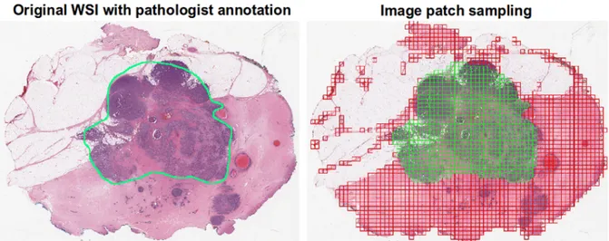
Figure 1.1: An example of whole slide image, with its grid decomposition in patches. It is visible the correspondence between a region of interest maually anotated and the patches that matches that region. From [13]

processes, the integration with other digitalized clinical workflows, and patients’ history, and most importantly the opening to applications of artificial intelligence.

The modern virtual microscopy discipline consists of scanning a complete microscope slide and creating a single high-resolution digital file, and it is typically referred as Whole Slide Imaging (WSI). The digitalization process is achieved capturing many small high-resolution image tiles or strips and then montaging them to create a full image of a histological section. The four key steps of this process are image acquisition (scansion), editing, and on-screen image visualization.

In the field of Digital Pathology (DP) an essential concept in image understanding is the magnification factor, which indicates the scale of representation of the image and allows dimension referencing. This factor is usually indicated as the magnification power of the microscope’s lenses used during the analysis. After the digitalization process, this original magnification factor is prone to change, depending on the resolution of the visualization screen. Therefore, image resolution is measured in µm per pixel, and it is set by the different composition of the acquisition chain, as the optical sensor and the lenses. Histological scanner are usually equipped with 20× or 40× objectives, which correspond to 0.5 and 0.25 mm/pixels resolution values. Lenses with 20× magnification factor are the most suitable for the great majority of histopathological evaluations, and it is the golden standard for scansions, for its good trade-off between image quality and time of acquisition. Scansions with 40× magnification could increase four-fold acquisition and processing time, final file’s dimension, and storage cost. A single WSI image, acquired with 20× will occupy more than 600 MB alone.

the standard primitive diagnosis phase in histopathological laboratories. This is primar-ily due to some disadvantages, like images’resolution, image compression’s artifacts, and auto-focusing algorithms, which plays a key role in the specimen interpretation. Fur-thermore, the scansion of histological samples is an additional step in the analysis which takes time. Despite the technological improvements the average time for the acquisition of a sample is around 5/10 minutes, depending on the number of slices in the slide, for just a single level of magnification. While in traditional histology, the pathologist has access to all the magnification levels at the same time. The real advantage, in fact, is in the long term. Once the images have been acquired they can be archived and consulted remotely almost instantaneously, helping clinical analysis and allowing remote assistance (telemedicine). Furthermore, the images now can be processed by artificial intelligence algorithms, allowing the application of technologies like Deep Learning which could rev-olutionize the research field, as already has been on many different disciplines in the scientific world.

In order to automatically process images of such big dimensions, as the ones obtained through WSI, it is necessary to subdivide them in smaller patches. The dimension of which should be big enough to allow interpretation and to preserve a certain degree of representability of the original image. In Figure 1.1 is shown an example of a whole slide image, with its grid decomposition in patches. If the patches are too small, it should be over-specified for a particular region of tissue, loosing its general features. This could lead the learning algorithm to misinterpretation. However, this is not an exclusive limit of digital pathology, for a human pathologist would be impossible too to make solid decisions on a too limited sample of tissue. After the subdivision in patches, a typical process for biomedical images is the so-called data augmentation of images, that is the process of creating re-newed images from the starting material through simple geometrical transformations, like translation, rotation, reflection, zoom in/out.

The analysis of histological images usually consists of detecting the different com-ponents in the samples and to recognize their arrangement as a healthy or pathological pattern. It is necessary to recognize every sign of the vitality of the cells, evaluating the state of the nucleus. There are many additional indicators to consider like the pres-ence of inflammatory cells or tumoral cells. Furthermore, samples which are taken from different part of the human body present completely different characteristics, and this increase greatly the complexity of the analysis. A reliable examination of a sample thus requires a careful inspection made by a highly qualified expert. The automatization of this procedure would be extremely helpful, giving an incredible boost both in timing and accessibility. However, this is not a simple task and in section 1.3.1 I will show some actual model for biomedical image processing in detail.

Figure 1.2: A sample of tissue from a retina (a part of the eye) stained with hematoxylin and eosin, cells’ nuclei are stained in blue-purple and extracellu-lar material is stained in pink.

1.1.1

Slides Preparation for Optic Microscopic Observation

In modern, as in traditional, histology regardless of the final support of the image the slide has to be physically prepared, starting from the sample of tissue. The slide preparation is a crucial step for histological or cytological observation. It is essential to highlight what needs to be observed and to immobilize the sample at a particular point in time and with characteristics close to those of its living state. There are five key steps for the preparation of samples [4]:

1) Fixation is carried out immediately after the removal of the sample to be observed. It is used to immobilize and preserve the sample permanently in as life-like state as possible. It can be performed immersing the biological material in a formalin solution or by freezing, so immersing the sample in a tissue freezing medium which is then cooled in liquid nitrogen.

2) Embedding if the sample has been stabilized in a fixative solution, this is the sub-sequent step. It consists in hardening the sample in a paraffin embedding medium, in order to be able to carry out the sectioning. It is necessary to dehydrate the sample beforehand, by replacing the water molecules in the sample with ethanol. 3) Sectioning Sectioning is performed using microtomy or cryotomy. Sectioning is an

important step for the preparation of slides as it ensures a proper observation of the sample by microscopy. Paraffin-embedded samples are cut by cross-section, using a

microtome, into thin slices of 5 µm. Frozen samples are cut using a cryostat. The frozen sections are then placed on a glass slide for storage at -80◦C. The choice of these preparation conditions is crucial in order to minimize the artifacts. Paraffin embedding is favored for preserving tissues; freezing is more suitable for preserving DNA and RNA and for the labeling of water-soluble elements or of those sensitive to the fixation medium.

4) Staining Staining increases contrasts in order to recognize and differentiate the dif-ferent components of the biological material. The sample is first deparaffinized and rehydrated so that polar dyes can impregnate the tissues. The different dyes can thus interact with the components to be stained according to their affinities. Once staining is completed, the slide is rinsed and dehydrated for the mounting step. Hematoxylin and eosin stain (H&E) is one of the principal tissue stains used in histology [45], and it is the most widely used stain in medical diagnosis and is often the gold standard [36]. H&E is the combination of two histological stains: hematoxylin and eosin. The hematoxylin stains cells’ nuclei blue, and eosin stains the extracellular matrix and cytoplasm pink, with other structures taking on different shades, hues, and combinations of these colors. An example of H&E stained is shown in Figure 1.2, in which we can see the typical color palette of a histological specimen.

1.1.2

Pancreas Microanatomy and Evidences of Neoplasms

The Pancreas is an internal organ of the human body, part of both the digestive system and the endocrine system. It acts as a gland with both endocrine and exocrine functions, and it is located in the abdomen behind the stomach. Its main endocrine duty is the secretion of hormones like insulin and glucagon which are responsible for the regulation of sugar levels in the blood. As a part of the digestive system instead, it acts as an exocrine gland secreting pancreatic juice, which has an essential role in the digestion of many different nutritional compounds. The majority of pancreatic tissue has a digestive role, and the cells with this role form clusters called acini around the small pancreatic ducts. The acinus secrete inactive digestive enzymes called zymogens into the small intercalated ducts which they surround, and then in the pancreatic blood vessels system [27]. In Figure 1.3 is shown a picture of the pancreas, with its structure and its placement in the human body. All the tissue is actually rich in other important elements as the islets of Langerhans that have an important role in the endocrine action of the pancreas. All over the structure is present a layer of connective tissue which are clearly visible in the traditional histological specimens.

There are many tumoral diseases involving pancreas, they represent one of the main causes of decease for cancer in occidental countries, and its incidence rate in Europe and the USA has risen significantly in the last decades. There are two main kinds of pancreatic neoplasms: endocrine and exocrine pancreatic tumors. The endocrine

Figure 1.3: A picture of pancreas’ structure in its physiological context. In this picture is clearly visible the macroscopic structure and the glandular organization at microscopic level.

pancreas neoplasms derive from the cells constituting the Langherans’ islets and are typically divided into functioning and non-functioning ones, depending on the capability of the organs to secrete hormones. Those diseases might be benign or malignant and they can have a different degree of aggressivity. Exocrine pancreatic tumors tough are the most frequent ones. Among those, the great majority of episodes are of malignant neoplasms, and in particular, the ductal adenocarcinoma is the most frequent form of disease, responsible alone for the 95% of the cases. From a macroscopic point of view, those tumors are characterized by an abundant fibrotic stroma1, which can represent over 50% of the tumor’s mass and it is responsible for the hard-ligneous tumor’s aspect. This disease is frequently associated to pancreatitis episodes.

From a microscopical point of view, this tumor is characterized by the presence of glandular structures, made by one or more layers of columnar or cuboidal epithelial cells embedded in fibrotic parenchyma. The histological inspection of a sample of pancreatic tissue allows us to grade the stadium of the disease. While analyzing a specimen the operator looks for some specific markers like the glandular differentiation in tubular and ductal structure, the degree of production of mucin, the percentage of cells in the mitotic phase, and the degree of tissue nuclear atypia. The evaluation of those characters allows us to assign a degree of development form I to III to the specific case of ductal

1_{Stroma is the part of a tissue or organ with a structural or connective role. It is made up of all the}

parts without specific functions of the organ like connective tissue, blood vessels, ducts, etc. The other part, the parenchyma, consists of the cells that perform the function of the tissue or organ.

adenocarcinoma.

During the microscopical analysis of a histological sample, there are other interesting markers to be evaluated, as a specific set of lesions which goes under the name of PanIN (Pancreatic Intraepithelial Neoplasia) and could not be appreciated with other diagnostic techniques. PanIN describes a wide variety of morphological modifications, differentiated on the degree of cytological atypia and architectural alterations [20]. A careful analysis of a histological sample of tissue after a biopsy is a fundamental step in the treatment of a patient.

1.1.3

Skin Microanatomy and Evidences of Neoplasms

Skin is the layer of soft, flexible outer tissue covering the body of a vertebrate animal, with the three main functions of protection, regulation, and sensation. Mammalian skin is composed of two primary layers: the epidermis, and the dermis. The epidermis is composed of the outermost layers of the skin. It forms a protective barrier over the body’s surface, responsible for keeping water in the body and preventing pathogens from entering. It is a stratified squamous epithelium, composed of proliferating basal and differentiated suprabasal keratinocytes. The dermis is the layer of skin beneath the epi-dermis that consists of connective tissue and cushions the body from stress and strain. The dermis provides tensile strength and elasticity to the skin through an extracellular matrix composed of collagen fibrils, microfibrils, and elastic fibers, embedded in hyaluro-nan and proteoglycans.

Melanoma is the most aggressive form of skin tumor. It is the second most fre-quent tumors in men under 50 years, and the third for women under 50 years, with over than 12.300 cases in Italy every year. Melanoma is considered nowadays a multifactorial pathology, which originates from the interaction between genetic susceptibility and en-vironmental exposure. The most important enen-vironmental risk factor is the intermittent solar exposure, for the genotoxic effect of ultraviolet rays on the skin. Different studies show also a strong correlation between the total number of nevi on the skin and the incidence of melanoma: among the subjects with familiar medical history of melanoma, the risk is greater for the subject affected by dysplastic nevus syndrome.

We can distinguish two separated phases in the growth of melanoma: the radial phase, in which the proliferation of malignant melanocytes is limited to the epidermis, and the vertical phase, where malignant melanocytes form nests or nodules in the dermis. The dermatological analysis should distinguish which specific type of melanoma is affecting the patient. There are many types of melanoma:

Superficial Spreading Melanoma : This is the most common subtype, and it rep-resents alone more than the 75% of all melanoma cases. These neoplasms show relatively large malignant melanocytes, inflammatory cells (epithelioid), and an abundance of cytoplasm.

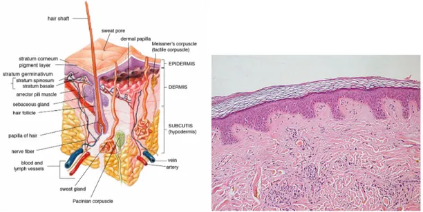
Figure 1.4: (left) Microanatomical description of a region of dermal tis-sue and all the interesting elements present in cutis, and subcutaneous layer. (right) An actual histological specimen from a sample of dermal tissue.

Lentigo Maligna Melanoma : It typically arises in photodamaged skin regions. Ne-plasmatic melanocytes are of polygonal shape, with hyperchromatic nuclei, and they are followed by a reduction in the cytoplasm.

Acral lentiginous melanoma : It typically arises on palmar, plantar, subungual, or mucosal surfaces. Melanocytes are usually arranged along the dermal-epidermal junction. The progression of this type of melanoma is characterized by the pres-ence of large junctional nests of atypical melanocytes, which are extended and hyperchromatic, with a shortage of cytoplasm.

Nodular Melanoma : By definition, this is the melanoma with a pure vertical growth. It is followed by the presence of numerous little tumoral nests of neoplastic melanocytes, with a high rate of mitotic state, arranged to form a single big nodule.

The careful examination of histological samples extracted from the tissue under anal-ysis is the most important step for the assessment of the actual form of neoplasms.

1.2

Introduction to Deep Learning

Deep Learning is part of the broader framework of Machine Learning and Artificial In-telligence. Indeed all the problems typically tackled using ML can also be addressed with DL techniques, for instance, regression, classification, clustering, and segmentation problems. We can think of DL as a universal methodology for iterative function ap-proximation with a great level of complexity. In the last decades, this technology has seen a frenetic diffusion and an incredible development, thanks to the always increasing available computational power, and it has become a staple tool in all sorts of scientific applications.

1.2.1

Perceptrons and Multilayer Feedforward Architecture

Like other artificial learning techniques, DL models aim to learn a relationship between some sort of input and a specific kind of output. In other words, approximating nu-merically the function that processes the input data and produces the desired response. For example, one could be interested in clustering data in a multidimensional features space, or in the detection of objects in a picture, or in text manipulation/generation. The function is approximated employing a greatly complex network of simple linear and non-linear mathematical operations arranged in a so-called Neural Network (typically with millions of parameters). The seed idea behind this discipline is to recreate the functioning of actual neurons in the human brain: their entangled connection system and their “ON/OFF” behavior [42].

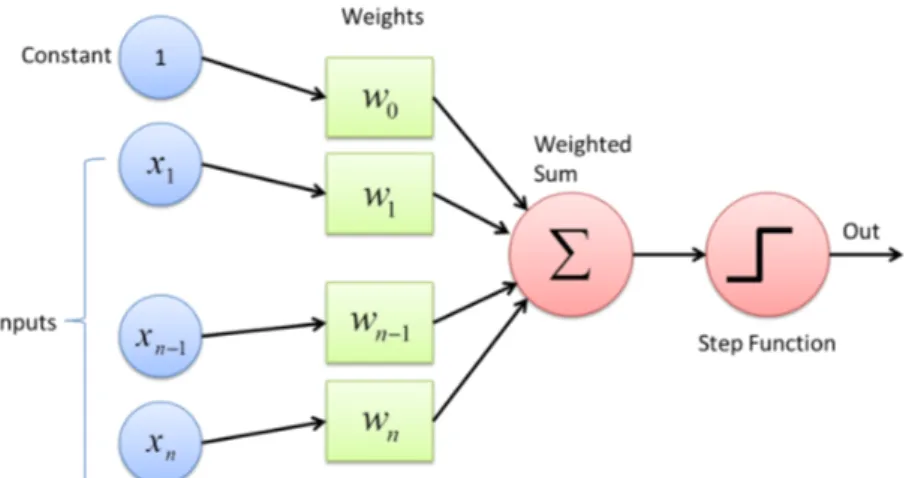
The fondamental unit of a neural network is called perceptron, and it acts as a digital counterpart of a human neuron. As shown in Figure 1.5 a perceptron collects in input a series on n numerical signals ~x = 1, x1, ..., xnand computes a linear wieghted combination

with the weights vectors ~w = w0, w1, ..., wn, where w0 is a bias factor:

f (~x, ~w) = χ(~x · ~w). (1.1) The results of this linear combination are given as input to a non-linear function χ(x) called the activation function. Typical choices as activation function are any sigmoidal function like sign(x) and tanh(x), but in more advanced applications other functions like ReLU [1] are used. The resulting function f (~x, ~w) has then a simple non linear behaviour. It produces a binary output: 1 if the weighted combination is high enough and 0 if it is low enough, with a smooth modulation in-between the two values.

The most common architecture for a NN is the so-called feed-forward architecture, where many individual perceptrons are arranged in chained layers, which take as input the output of previous layers along with a straight information flux. More complex ar-chitectures could implements also recursive connection, linking a layer to itself, but it should be regarded as sophistication to the standard case. There are endless possibilities

Figure 1.5: Schematic picture of a single layer perceptron. The input vector is linearly combined with the bias factor and sent to an activation function to produce the numerical ”binary” output.

of combination and arrangement of neurons inside a NN’s layer, but the most simple ones are known as fully-connected layers, where every neuron is linked with each other neuron of the following layer, as shown in Figure 1.6. Each connection has its weight, which contributes to modulate the overall combination of signals. The training of a NN consists then in the adjustment and fine-tuning of all the network’s weights and param-eters through iterative techniques until the desired precision in the output generation is reached.

Although a fully connected network represents the simplest linking choice, the inser-tion of each weight increases the number of overall parameters, and so the complexity of the model. Thus we want to create links between neurons smartly, rejecting the less useful ones. Depending on the type of data under analysis there are many different estab-lished typologies of layers. For example, in the image processing field, the most common choice is the convolutional layer, which implements a sort of discrete convolution on the input data, as shown in Figure 1.7. While processing images, the convolution operation confers to the perception of correlation between adjacent pixels of an image and their color channels, allowing a sort of spatial awareness. Furthermore, the majority of tradi-tional computer vision techniques are based on the discrete convolution of images, and on the features extracted from them.

As a matter of principle a NN with just two successive layers, which is called a shallow network, and with an arbitrary number of neurons per layer, can approximate arbitrary well any kind of smooth enough function [33]. However, direct experience suggests that networks with multiple layers, called deep networks, can reach equivalent results exploiting a lower number of parameters overall. This is the reason why this discipline goes under the name of deep learning: it focuses on deep networks with up

Figure 1.6: Schematic representation of a fully connected (or dense) layer. Every neuron from the first layer is connected with every output neuron. The link thickness represent the absolute value of the combination weight for that particular value.

to tents of hidden layers. Such deep structures allow the computation of what is called deep features, so features of the features of the input data, that allows the network to easily manage concepts that would be bearly understandable for humans.

1.2.2

Training Strategies in Deep Learning

Depending on the task the NN is designed for, it will have a different architecture and number of parameters. Those parameters are initialized to completely random values, tough. The training process is exactly the process of seeking iteratively the right values to assign to each parameter in the network in order to accomplish the task. The best start to understanding the training procedure is to look at how a supervised problem is solved. In supervised problems, we start with a series of examples of true connections between inputs and correspondent outputs and we try to generalize the rule behind those examples. After the rule has been picked up the final aim is to exploit it and to apply it to unknown data, so the new problem could be solved. In opposition to the concept of supervised problems, there are the unsupervised problems, where the algorithm does not try to learn a rule from a practical example but try to devise it from scratch. A task typically posed as unsupervised is clustering, when different data are separated in groups based on the values of their features in the feature space. Usually, only the number of groups is taken in input from the algorithm, and the subdivision is completely performed by the machine. However, in the real world, there are many different and creative shapes

Figure 1.7: Schematical representation of a convolutional layer. The input data are processed by a window kernel that slides all over the image. This operation can recreate almost all the traditional computer vision techniques, and can overcome them, creating new operations, which would be unthinkable to hand-engineered.

between pure supervised and pure unsupervised learning, based on the actual availability of data and specific limitations to the individual task.

An interesting mention in this regard should be made about semi-supervised learning, which is typically used in biomedical applications. This learning technique combines a large quantity of unlabeled data during training with a limited number of pre-labeled example. The blend between data can produce a considerable improvement in learning accuracy and leading to better results with respect to pure unsupervised techniques. The typical situation of usage of this technique is when the acquisition of labeled data requires a highly trained human agent (as an anatomopathologist) or a complex physical experiment. The actual cost of building entire and suitable fully labeled training sets in these situations would be unbearable, and semi-supervised learning comes in great practical help.

Another important training technique which worth mentioning is the so-called cur-riculum learning [5]. This is a learning technique inspired by the typical learning curve of human beings and animals, that are used to resolve problems of always increasing difficulty while learning something new or a new skill. The example presented to the Neural Network are not randomly presented but organized in a meaningful order which illustrates gradually more concepts, and gradually more complex ones. The experiments show that through curriculum learning significant improvements in generalization can be achieved. This approach has both an effect on the speed of convergence of the training

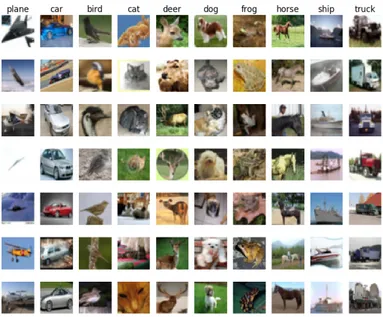
Figure 1.8: Sample grid of images from the CIFAR10 dataset. Each one of the 32 × 32 image is labeled with one of the ten classes of objects: plane, car, bird, cat, deer, dog, frog, horse, ship, truck.

process to a minimum and, in the case of non-convex criteria, on the quality of the local minima obtained. This technique is of particular interest for this work: the generated images, which will be shown in section 3.3 , will offer a segmentation task much less complex respect to the analysis of real histological tissue. In the view of training a DL-based model the abundantly produced images can be used for the preliminary phase of training, setting aside the more complex and more valuable hand-labeled images for the finalization of the training process.

1.2.3

Training Algorithms - Error Back-Propagation

A good example of supervised problems tough is the classification of images. Let’s assume we have a whole dataset of pictures of different objects (as cats, dogs, cars, etc.) like the CIFAR10 [23] dataset. This famous dataset is made of over 60K labeled colored images 32×32 divided into 10 categories of objects as shown in Figure 1.8. We could be interested in the creation of a NN able to assign at every image its belonging class. This NN could be arbitrarily complex but it certainly will take as input a 32×32×3 RGB image and the output will be the predicted class. A typical output for this problem would be a probability distribution over all the 10 classes like:

~ p = (p1, p2, . . . , p10), (1.2) 10 X i=1 pi = 1, (1.3)

and it should be compared with the true label, that is represented just as a binary sequence ~t with the bit correspondent to the belonging class set as 1, and all the others value set to 0:

~t = (0, 0, . . . , 1, . . . , 0, 0). (1.4) Every time an image is given to the model an estimate of the output is produced. Thus, we need to measure the distance between that prediction and the true value, to quantify the error made by the algorithm and try to improve the model’s predictive power. The functions used for this purpose are called loss functions. The most common choice is the Mean Squared Error (MSE) function that is simply the averaged L2 _norm

of the difference vector between ~p and ~t: M SE = 1 n n X i=0 (ti− pi)2. (1.5)

Let’s say the NN under training has L consecutive layers, each one with its activation function fk and its weights vector ~wk, hence the prediction vector ~p could be seen as the result of the concesutive, nested, application through all the layers:

~

p = fL( ~wL· (fL−1_{( ~w}L−1_{· ... · f}1_{( ~w}1_{· ~x)))). (1.6)}

From both equations 1.5 and 1.6 it is clear that the loss function could be seen as a function of all the weights vectors of every layer of the network. So if we want to reduce the distance between the NN prediction and the true value we need to modify those weights to minimize the loss function. The most established algorithm to do so for a supervised task in a feed-forward network is the so-called error back-propagation.

The back-propagation method is an iterative technique that works essentially com-puting the gradient of the loss function with respect to the weights using the derivative chain rule and updating by a small amount the value of each parameter to lower the overall loss function at each step. Each weight is moved counter-gradient, and summing all the contribution to every parameter the loss function approaches its minimum. In equation 1.7 is represented the variation applied to the jth weight in the ith layer in a single step of the method:

∆wij = −η

∂E ∂wij

where E is the error function, and η is the learning coefficient, that modulate the effect of learning through all the training process. This iterative procedure is applied completely to each image in the training set several times, each time the whole dataset is reprocessed is called an epoch. The great majority of the dataset is exploited in the training phase to keep running this trial and error process and just a small portion is left out (typically 10% of the data) for a final performance test.

The loss function shall inevitably be differentiable, and its behavior heavily influences the success of the training. If the loss function presents a gradient landscape rich of local minima the gradient descent process would probably get stuck in one of them. More sophisticated algorithms capable of avoiding this issue have been devised, with the insertion of some degree of randomness in them, as the Stochastic Gradient Descent algorithm, or the wide used Adam optimizer [22].

While Error-Back Propagation is the most established standard in DL applications, it suffers from some problems. The most common one is the so-called vanishing or explod-ing gradient issue, which is due to the iterative chain derivation through all the nested level of composition of the function. Without a careful choice of the right activation function and the tuning of the learning hyper-parameters, it is very easy to bump into this pitfall. Furthermore, the heavy use of derivation rises the inability to handle non-differentiable components and hinders the possibility of parallel computation. However, there are many alternative approaches to network learning besides EBP. The Minimiza-tion with Auxiliary Variables (MAV) method builds upon previously proposed methods that break the nested objective into easier-to-solve local subproblems via inserting auxil-iary variables corresponding to activations in each layer. Such a method avoids gradient chain computation and the potential issues associated with it [10]. A further alterna-tive approach to train the network is the Local Error Signals (LES), which is based on layer-wise loss functions. In [30], is shown that layer-wise training can approach the state-of-the-art on a variety of image datasets. It is used a single-layer sub-networks and two different supervised loss functions to generate local error signals for the hidden layers, and it is shown that the combination of these losses helps with optimization in the context of local learning.

The training phase is the pulsing heart of a DL model development and it could take even weeks on top-level computers for the most complicated networks. In fact, one of the great limits to the complexity of a network during the designing phase is exactly the available computational power. There are many more further technical details necessary for proper training, the adjustment of which can heavily impact the quality of the algorithm. However, after the training phase, we need to test the performance of the NN. This is usually done running the trained algorithm on never seen before inputs (the test dataset) and comparing the prediction with the ground-truth value. A good way to evaluate the quality of the results is to use the same function used as the loss function during the training, but there is no technical restriction to the choice of this quality metric. The average score on the whole test set is then used as a numerical score for

the network, and it allows straightforward comparison with other models’ performances, trained for the same task. All this training procedure is coherently customized to every different application, depending on which the problem is posed as supervised or not and depending on the more or less complex network’s architecture. The leitmotif is always finding a suitable loss function that quantifies how well the network does what it has been designed to do and trying to minimize it, operating on the parameters that define the network structure.

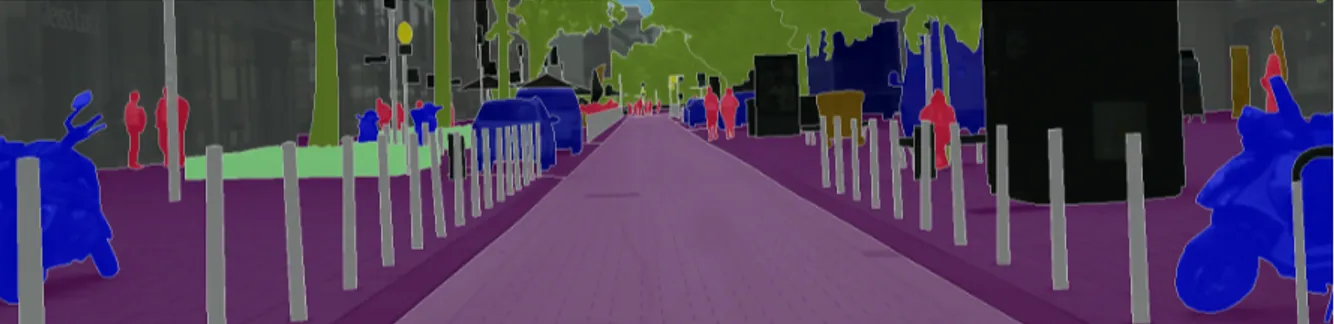
Figure 1.9: Example of the resulting segmentation mask of an image of an urban landscape. Every interesting object of the image is detected and a solid color region replaces it in the segmentation mask. Every color corresponds to a different class of objects, for example, persons are highlighted in magenta and scooters in blue. The shape and the boundaries of every region should match as precisely as possible the edges of the objects.

1.3

Deep Learning-Based Segmentation Algorithms

In digital image processing, image segmentation is the process of recognizing and sub-dividing an image into different regions of pixels that show similar features, like color, texture, or intensity. Typically, the task of segmentation is to recognize the edges and boundaries of the different objects in the image and assigning a different label to every detected region. The result of the segmentation process is an image with the same dimen-sions of the starting one made of solid color regions, representing the detected objects. This image is called segmentation mask. In Figure 1.9 is shown an example of segmenta-tion of a picture of an urban landscape: different colors are linked to different classes of objects like persons in magenta and scooters in blue. This technology has a significant role in a wide variety of application fields such as scene understanding, medical image analysis, augmented reality, etc.

A relatively easy segmentation problem, and one of the first to be tackled, could be distinguishing an object from the background in a grey-scale image, like in Figure 1.10. The easiest technique to perform segmentation in this kind of problem is based on thresholding. Thresholding is a binarization technique based on the image’s grey-level histogram: to every pixel with luminosity above that threshold is assigned the color white, and vice versa the color black. However, this is a very primitive, yet very fast method, and it manages poorly complex images or images with un-uniformity in the background.

A lot of other traditional techniques improve this first segmentation method [11]. Some are based on the object’s edges recognition, exploiting the sharp change in lumi-nosity typically in correspondence of the boundary of a shape. Other techniques exploit instead a region-growing technology, according to which some seed region markers are

Figure 1.10: Example of the resulting segmentation mask of an image of a fingeprint obtained trhough a thresholding algorithm. The result is not ex-tremely good, but this techinque is very easy to implement and runs very quickly.

scattered on the image, and the regions corresponding to the objects in the image are grown to incorporate adjacent pixels with similar properties.

Every development of traditional computer vision or of Machine Learning-based seg-mentation algorithm suffers from the same, inevitable limitation. In every one of these techniques a human operator should precisely decide during the designing phase which features to extract from the data and how to process them for the rest of the analysis: typical features that are used are different directional derivatives in the image plane, image entropy, and luminosity distribution among the color channels. There is thus an intrinsic limitation in the human comprehension of those quantities and in the possible way to process them. The choice is made on the previous experimental results in other image processing works, and on their theoretical interpretation. Neural Networks instead are relieved from this limitation, allowing themselves to learn which features are best suited for the task and how they should be processed during the training phase. The complexity is then moved on to the design of the DL model and on its learning phase rather than on the hand-engineering design of the features to extract. In Figure 1.11 an example of high-level feature extracted from a DL model trained for the segmentation of nuclei in a histological sample. The model learns the typical pattern of arrangement of nuclei, which would have been impossible to describe equally in advance.

1.3.1

State of the Art on Deep Learning Segmentation

In a similar way to many other traditional tasks, also for segmentation, there has been a thriving development lead by the diffusion of deep learning, that boosted the perfor-mances resulting in what many regards as a paradigm shift in the field [28].

In further detail, image segmentation can be formulated as a classification problem of pixels with semantic labels (semantic segmentation) or partitioning of individual objects (instance segmentation). Semantic segmentation performs pixel-level labeling with a set

Figure 1.11: (A) An extract from an histological samples, used as input image for the model. (B) The exact segmentation mask. (C) Example of accentuated features during the training: (1-4) for back-ground recognition, (5-8) for nuclei detection. From [2].

of object categories (e.g. boat, car, person, tree) for all the pixels in the image, hence it is typically a harder task than image classification, which requires just a single label for the whole image. Instance segmentation extends semantic segmentation scope further by detecting and delineating each object of interest in the image (e.g. partitioning of individual nuclei in a histological image).

There are many prominent Neural Network architectures used in the computer vision community nowadays, based on very different ideas such as convolution, recursion, di-mensionality reduction, and image generation. This section will provide an overview of the state of the art of this technology and will dwell briefly on the details behind some of those innovative architectures.

Recurrent Neural Networks (RNNs) and the LSTM

The typical application for RNN is processing sequential data, as written text, speech or video clips, or any other kind of time-series signal. In this kind of data, there is a strong dependency between values at a given time/position and values previously processed. Those models try to implement the concept of memory weaving connections, outside the main information flow of the network, with the previous NN’s input. At each time-stamp, the model collects the input from the current time Xi and the hidden state from the previous step hi−1 and outputs a

target value and a new hidden state (Figure 1.12). Typically RNN cannot manage easily long-term dependencies in long sequences of signals. There is no theoretical limitation in this direction, but often it arises vanishing (or exploding) gradient problematics during the training phase. A specific type of RNN has been designed

Figure 1.12: Example of the structure of a simple Recurrent Neural Network from [28].

to avoid this situation, the so-called Long Short Term Memory (LSTM) [19]. The LSTM architecture includes three gates (input gate, output gate, forget gate), which regulate the flow of information into and out from a memory cell, which stores values over arbitrary time intervals.

Encoder-Decoder and Auto-Encoder Models

Encoder-Decoder models try to learn the relation between an input and the corre-sponding output with a two steps process. The first step is the so-called encoding process, in which the input x is compressed in what is called the latent-space rep-resentation z = f (x). The second step is the decoding process, where the NN predicts the output starting from the latent-space representation y = g(z). The idea underneath this approach is to capture in the latent-space representation the underlying semantic information of the input that is useful for predicting the out-put. ED models are widely used in image-to-image problems (where both input and output are images) and for sequential-data processing (like Natural Language Processing, NLP). In Figure 1.13 is shown a schematic representation of this ar-chitecture. Usually, these model follow a supervised training, trying to reduce the reconstruction loss between the predicted output and the ground-truth output pro-vided while training. Typical applications for this technology are image-enhancing techniques like de-noising or super-resolution, where the output image is an im-proved version of the input image, or image generation problems (e.g. plausible new human faces generation) in which all the properties which define the type of image under analysis should be learned in the representation latent space.

Generative Adversarial Networks (GANs)

The peculiarity of Generative Adversarial Network (GAN) lies in its structure. It is actually made of two distinct and independent modules: a generator and a discriminator, as shown in Figure 1.14. The first module G, responsible for the generation, typically learns to map a prior random distribution of input z to a

Figure 1.13: Example of the structure of a simple Encoder-Decoder Neural Network from [28].

target distribution y, as similar as possible to the target G = z → y (i.e. almost any kind of image-to-image problem could be addressed with GANs, as in [21]). The second module, the discriminator D, instead is trained to distinguish between real and fake images of the target category. These two networks are trained alternately in the same training process. The generator tries to fool the discriminator and vice versa. The name adversarial is actually due to this competition within different parts of the network. The formal manner to set up this adversarial training lies in the accurate choice of a suitable loss function, that will look like:

LGAN = Ex∼pdata(x)[logD(x)] + Ez∼pz(z)[log(1 − D(G(z)))].

The GAN is thus based on a min-max game between G and D. D aims to reduce the classification error in distinguishing fake samples from real ones, and as a consequence maximizing the LGAN. On the other hand, G wants to maximize the

D’s error, hence minimizing LGAN. The result of the training process is the trained

generator G∗, capable of produce an arbitrary number of new data (images, text, or whatever else):

G∗ = arg minGmaxDLGAN.

This peculiar architecture has yielded several interesting results and it has been developed in many different directions, with influences and contaminations with other architectures [21].

Convolutional Neural Networks (CNNs)

As stated before CNNs are a staple choice in image processing DL applications. They mainly consist of three types of layers:

i convolutional layers, where a kernel window of parameters is convolved with the image pixels and produce numerical features maps.

ii nonlinear layers, which apply an activation function on feature maps (usually element-wise). This step allows the network to introduce non-linear behavior and then increasing its modeling capabilities.

Figure 1.14: Schematical representation of a Generative Adversarial Net-works, form [28].

iii pooling layers, which replace a small neighborhood of a feature map with some statistical information (mean, max, etc.) about the neighborhood and reduce the spatial resolution.

Given the arrangement of successive layers, each unit receives weighted inputs from a small neighborhood, known as the receptive field, of units in the previous layer. The stack of layers allows the NN to perceive different resolutions: the higher-level layers learn features from increasingly wider receptive fields. The leading computational advantage given by CNN architecture lies in the sharing of kernels’ weights within a convolutional layer. The result is a significantly smaller number of parameters than fully-connected neural networks. In section 2.7 will be shown a particular application of this architecture, known as style-transfer network, which is a particular algorithm capable of implanting the visual texture of a style image onto the content of a different image, producing interesting hybrid images. Some of the most notorious CNN architectures include: AlexNet [24], VGGNet [41], and U-Net [35].

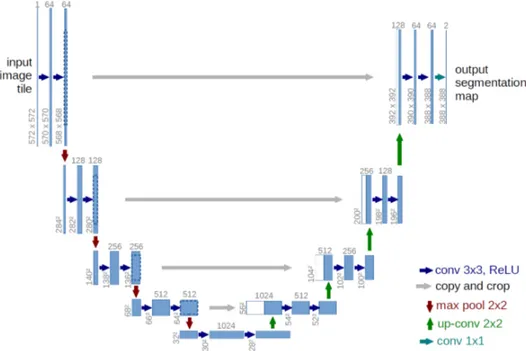
For this work, U-net architecture is particularly interesting. The U-net model was initially developed for biomedical image segmentation, and in its structure reflects char-acteristics of both CNN and Encoder-Decoder models. Ronneberger et al.[35] proposed this model for segmenting biological microscopy images in 2015. The U-Net architecture is made of two branches, a contracting path to capture context, and a symmetric expand-ing path (see Figure 1.15). The down-samplexpand-ing flow is made of a Fully Convolutional Network (FCN)-like architecture that computes features with 3 × 3 kernel convolutions. On the other hand, the up-sampling branch exploits up-convolution operations (or de-convolution), reducing the number of feature maps while increasing their dimensions. Another characteristic of this architecture is the presence of direct connections between layers of a similar level of compression in compressing and decompressing branches. Those links allow the NN to preserve spatial and pattern information. The Network flow eventually ends with a 1 × 1 convolution layer responsible for the generation of the segmentation mask of the input image.

Figure 1.15: Scheme of the typical architecture of a U-net NN. This par-ticular model was firstly proposed by Ronneberger et al. in [35].

A recent example of a practical application of a CNN to histological images could be found in [29]. In this work the Inception v3 is trained on hand-labeled samples of pancreatic tissue (like in Figure 1) to recognize tumoral regions from healthy ones in a pancreatic tissue specimen treated with Ki67 staining. The Inception v3 [34] network is a deep convolutional network developed by Google, trained for object detection and image classification on the ImageNet dataset [15]. Recognition of the tumoral region of Ki67 stained pancreatic tissue samples is based on the detection and counting of some specific marker cells. In Figure 1.16 is shown a pair of the original image and the computed segmentation mask, which label in red tumoral regions and green the healthy ones. This work is based on a technique called transfer learning, which consists of the customization and specialization of a pre-trained NN previously trained for similar, but essentially different, tasks. The final part of the training of this version of Inception v3 has been performed of a dataset of 33 whole slide images of Ki67 stained neuroendocrine tumor biopsies acquired from 33 different patients, digitized with a 20× magnification factor and successively divided in 64×64 patches.

1.3.2

Image Segmentation Datasets

Besides the choice of suitable architecture the most important aspect while developing a NN is the dataset to use for the training process. Let’s confine the discussion only to

Figure 1.16: (left) Original image of a Ki67 stained pancreatic tissue sam-ple, (right) the corresponding segmentation mask, which label in red tumoral regions and in green the healthy ones. From [29].

Figure 1.17: An example image from the PASCAL dataset and its corre-sponding segmentation mask [17].

image-to-image problems, like segmentation problems. There are a lot of widely used datasets, but I want to mention just a few of them to give the idea of their typical characteristics.

A good example of segmentation is the Cityscapes dataset [12], which is a large-scale database with a focus on semantic understanding of urban street scenes. The dataset is made of video sequences from the point of view of a car in the road traffic, from 50 different cities in the world. The clips are made of 5K frames, labeled with extremely high quality at pixel-level and an additional set of 20K weakly-annotated frames. Each pixel in the segmentation mask contains the semantic classification, among over 30 classes of objects. An example of an image from this dataset is shown in Figure 1.9.

The PASCAL Visual Object Classes (VOC) [17] is another of the most popular datasets in computer vision. This dataset is designed to support the training of algo-rithms for 5 different tasks: segmentation, classification, detection, person layout, and action recognition. In particular, for segmentation, there are over 20 classes of labeled objects (e.g. planes, bus, car, sofa, TV, dogs, person, etc.). The dataset comes divided into two portions: training and validation, with 1,464 and 1,449 images, respectively. In Figure 1.17 is shown an example of an image and its corresponding segmentation mask.

As the last mention, I would report the ImageNet project [15], which is a large visual database designed for use in visual object recognition software research. It consists of more than 14 million images that have been hand-annotated by the project to indicate what objects are pictured and in at least one million of the images, bounding boxes are also provided. ImageNet contains more than 20,000 categories of objects. Since 2010, the ImageNet project runs an annual software contest, the ImageNet Large Scale Visual Recognition Challenge (ILSVRC), where software programs compete to correctly classify and detect objects and scenes. This kind of competition is very important for the research field, as it inspires and encourages the development of new models and architectures.

It is worth mentioning that in the medical image processing domain typically the available dataset is definitely not that rich and vast (that is actually the seed of this work) and thus many techniques of data augmentation have been devised, to get the best out of the restricted amount of material. Generally, data augmentation manipu-lates the starting material applying a set of transformation to create new material, like rotation, reflection, scaling, cropping and shifting, etc. Data augmentation has been proven to improve the efficacy of the training, making the model less prone to over-fitting, increasing the generalization power of the model, and helping the convergence to a stable solution during the training process.

Chapter 2

Technical Tools for Model

Development

As mentioned in the introduction, this project wants to produce synthetic histological images paired with their corresponding segmentation mask, to train Neural Networks for the automatization of real histological images analysis. The production of artificial images passes through the processing of a three-dimensional, virtual model of a histo-logical structure, which is the heart of this thesis work. The detailed description of the development of the two proposed histological models will follow the present chapter and will occupy the entire chapter 3. Here I will dwell, instead, on every technical tool em-ployed during the models’ designing phase. From the practical point of view, this project is quite articulated and the development has required the harmonization of many dif-ferent technologies, tools, and code libraries. The current chapter should be seen as a theoretical complement for chapter 3, and its reading is suggested to the reader for any theoretical gap or for any further technical deepening. The reader already familiar with those technical tools should freely jump to the models’ description.

All the code necessary for the work has been written in a pure Python environment, using several already established libraries and writing by myself the missing code for some specific applications. I decided to code in Python given the thriving variety of available libraries geared toward scientific computation, image processing, data analysis, and last but not least for its ease of use (compared to other programming languages). In each one of the following subsections, I will mention the specific code libraries which have been employed in this project for every technical necessity.

2.1

Quaternions

Quaternions are, in mathematics, a number system that expands to four dimensions the complex numbers. They have been described for the first time by the famous

mathemati-cian William Rowan Hamilton in 1843. This number system define three independent imaginary units i, j, k as in (2.1), which allows the general representation of a quaternion q is (2.2) and its inverse q−1 (2.3) where a, b, c, d are real numbers:

i2 = j2 = k2 = ijk = −1, (2.1)

q = a + bi + cj + dk, (2.2)

q−1 = (a + bi + cj + dk)−1= 1

a2_{+ b}2_{+ c}2_{+ d}2 (a − bi − cj − dk). (2.3)

Furthermore, the multiplication operation between quaternions does not benefit from commutativity, hence the product between basis elements will behave as follows:

i · 1 = 1 · i = i, j · 1 = 1 · j = j, k · 1 = 1 · k = k (2.4) i · j = k, j · i = −k

k · i = j, i · k = −j j · k = i, k · j = −i.

This number system has plenty of peculiar properties and applications, but for this project, quaternions are important for their ability to represent, in a very convenient way, rotations in three dimensions. The particular subset of quaternions with vanishing real part (a = 0) has a useful, yet redundant, correspondence with the group of rotations in tridimensional space SO(3). Every 3D rotation of an object can be represented by a 3D vector ~u: the vector’s direction indicates the axis of rotation and the vector magnitude |~u| express the angular extent of rotation. However, the matrix operation which expresses the rotation around an arbitrary vector ~u it is quite complex and does not scale easily for multiple rotations [7], which brings to very heavy and entangled computations.

Using quaternions for expressing rotations in space, instead, it is very convinient. Given the unit rotation vector ~u and the rotation angle θ, the corresponding rotation quaternion q becomes (2.6):

~

u = (ux, uy, uz) = uxi + uyj + uzk, (2.5)

q = eθ2(uxi+uyj+uzk)= cosθ

2 + (uxi + uyj + uzk) sin θ 2, (2.6) q−1 = cosθ 2 − (uxi + uyj + uzk) sin θ 2, (2.7)

where in (2.6) we can clearly see a generalization of the Euler’s formula for the exponential notation of complex numbers, which hold for quaternions. It can be shown