Statistical methods for the analysis of DNA sequences: application to dinucleotide distribution in the human genome

(1)

Alma Mater Studiorum · Universit`

a di Bologna

Scuola di Scienze

Corso di Laurea Magistrale in Fisica

Statistical methods for the analysis of DNA

sequences: application to dinucleotide

distribution in the human genome

Relatore:

Prof.

Daniel Remondini

Correlatore:

Dott.

Giampaolo Cristadoro

Presentata da:

Giulia Paci

Sessione II

Anno Accademico 2013/14

(2)

(3)

Abstract

Questa tesi si inserisce nell’ambito delle analisi statistiche e dei metodi sto-castici applicati all’analisi delle sequenze di DNA. Nello specifico il nostro la-voro è incentrato sullo studio del dinucleotide CG (CpG) all’interno del genoma umano, che si trova raggruppato in zone specifiche denominate CpG islands. Queste sono legate alla metilazione del DNA, un processo che riveste un ruolo fondamentale nella regolazione genica. La prima parte dello studio è dedicata a una caratterizzazione globale del contenuto e della distribuzione dei 16 di-versi dinucleotidi all’interno del genoma umano: in particolare viene studiata la distribuzione delle distanze tra occorrenze successive dello stesso dinucleotide lungo la sequenza. I risultati vengono confrontati con diversi modelli nulli: sequenze random generate con catene di Markov di ordine zero (basate sulle frequenze relative dei nucleotidi) e uno (basate sulle probabilità di transizione tra diversi nucleotidi) e la distribuzione geometrica per le distanze. Da questa analisi le proprietà caratteristiche del dinucleotide CpG emergono chiaramente, sia dal confronto con gli altri dinucleotidi che con i modelli random. A se-guito di questa prima parte abbiamo scelto di concentrare le successive analisi in zone di interesse biologico, studiando l’abbondanza e la distribuzione di CpG al loro interno (CpG islands, promotori e Lamina Associated Domains). Nei primi due casi si osserva un forte arricchimento nel contenuto di CpG, e la dis-tribuzione delle distanze è spostata verso valori inferiori, indicando che questo dinucleotide è clusterizzato. All’interno delle LADs si trovano mediamente meno CpG e questi presentano distanze maggiori. Infine abbiamo adottato una rap-presentazione a random walk del DNA, costruita in base al posizionamento dei dinucleotidi: il walk ottenuto presenta caratteristiche drasticamente diverse all’interno e all’esterno di zone annotate come CpG island. Riteniamo pertanto che metodi basati su questo approccio potrebbero essere sfruttati per miglio-rare l’individuazione di queste aree di interesse nel genoma umano e di altri organismi.

(4)

(5)

Introduction

There’s real poetry in the real world. Science is the poetry of reality. -Richard Dawkins

Methylation of DNA is one of the most important epigenetic processes, some-times referred to as the “fifth base” for its key role in functions such as gene regulation. CpG islands are important genomic regions, which are believed to be protected from methylation but can also show aberrant methylation pat-terns in different diseases, including cancer; it is therefore important to obtain “maps” of these regions in order to develop appropriate assays to monitor DNA methylation where this could be linked to diseases.

However, since the first formal definition of a CpG island, given by Gardner, Gardiner and Frommer in 1987 [18], many alternative definitions and algorithms for CGI annotation have been proposed (see for example [42] and [24]), and the matter is still much debated.

As physicists approaching a biological problem new to us, we decided to take a step back and first of all aim at characterising in detail the positioning of CpG dinucleotides in the whole genome, comparing them with the different dinucleotides and with appropriate random models. To do this, we employed a method based on the computation of distances between successive occurrences of dinucleotides and we considered a zeroth and first order Markov chain models for random reference sequences.

(8)

The first part of our work is focused on a global analysis of dinucleotides in the whole human genome: we compare the relative frequencies and the distance dis-tributions of all 16 dinucleotides with each other and with reference sequences generated with both a Markov 0 and Markov 1 models, as well as a null model of distance distributions given by the geometric distribution. We then focus on genomic regions of interest, specifically CpG islands (we compare two differ-ent annotations), promoters and LADs (Lamina Associated Domains, regions of DNA which bind to the nuclear membrane and control the three dimensional structure of the DNA sequence) to gather insight on the mutual relationship between these areas and their CpG content and distributions. In the final part of this thesis we employ a random walk based representation of the DNA se-quence, which is constructed based on dinucleotide positioning, and we discuss the possibility of using simple methods based on DNA walks for the search of candidate CpG islands.

In the first chapter we introduce the biological background and motivation of this work, with a focus on DNA methylation and the concept of CpG islands. The second chapter is devoted to the main methods employed in our study, namely Markov chain models, inter-dinucleotide distance distribution analysis and the random walk representation of DNA. In the third chapter we illustrate the results of the characterisation of dinucleotide abundances and distribution in the whole genome. The fourth chapter is focused on the analysis inside genomic regions of interest and on the results of our DNA walk representation applied to CpG islands.

(9)

CHAPTER

1

CpG islands and DNA methylation

In this chapter we briefly review the biological background of this work. In the first two sections we give an overview of the human genome and of the most important sequencing techniques which allow the analysis of the DNA bases sequence. We then give a brief description of the methylation process in DNA, which is an important epigenetic modification and the main reason for the interest in CpG dinucleotides, the subject of this study. In the last section we describe the main definitions of CpG islands and we give a survey of methods and algorithms for CpG islands annotation present in literature.

1.1 The human genome

In all living organisms hereditary information is stored, transmitted and expressed with the help of nucleic acids DNA (deoxyribonucleic acid) and RNA (ribonucleic acid). DNA is the genetic material that organisms inherit from their parent: it provides directions for its own replication, directs RNA synthesis and, through RNA, controls protein synthesis.

DNA and RNA composition and structure

Nucleic acids are polymers, constituted of monomers called nucleotides. Each nucleotide is composed of a phosphate group, a sugar (deoxyribose in DNA, ribose in DNA) and a nitrogenous bases. There are two families of

(10)

nitrogenous bases: pyrimidines and purines. The first ones include cytosine, thymine and uracil (which is present in RNA instead of T) and are character-ized by one six-membered ring of carbon and nitrogen atoms. Purines, which are larger molecules formed by a six-membered ring fused to a five-membered ring, include adenine and guanine (see Figure 1.1b). In the polymer structure, adjacent nucleotides are joined by a phosphodiester bond: a phosphate group links the sugars of two nucleotides. This bonding results in a backbone with a repeating pattern of sugar-phosphate units characterized by an intrinsic direc-tionality: one end has a phosphate attached to the 5’ carbon, whereas the other has a hydroxyl group on a 3’ carbon (see Figure 1.1a).

RNA molecules usually exist as single polynucleotide chains, on the other hand DNA molecules have two polynucleotides, or strands, that spiral around an imaginary axis, forming a double helix structure (see Figure 1.2). The two strands are antiparallel, with sugar-phosphate backbones on the outside of the double helix running in the 5’-3’ direction opposite from each other. The ni-trogenous bases are paired in the interior of the helix, and hydrogen bonds between them hold the two strands together (see Figure1.2). Only certain bases in the double helix are compatible with each other: adenine always pairs with thymine by two hydrogen bonds and cytosine with guanine by three hydrogen bonds. The two strands are therefore complementary: if we were to read the sequence of bases along one strand of the double helix, we would know the se-quence of bases along the other strand. This unique feature of DNA allows the creation of two identical copies of each DNA molecule in a cell that is preparing to divide, making daughter cells genetically identical to the parent. Base pair-ing also occurs in RNA among bases in two different RNA molecules or on the same molecule: for example it is responsible for the three-dimensional functional structure of transfer RNA.

1.2 DNA sequencing: history and techniques

The goal of DNA sequencing is the determination of the precise order of nucleotides within a DNA molecule: this knowledge is essential for the advance-ment of biological and medical research, and can help the understanding of many diseases, for example with the identification of oncogenes and mutations linked to different forms of cancer. The main efforts towards the sequencing of the Human Genome started in 1990 with the launch of the Human Genome Project through funding from the the National Institutes of Health (NIH) and

(11)

1.2. DNA SEQUENCING: HISTORY AND TECHNIQUES 5

(a) (b)

Figure 1.1: (a) Structure of a polynucleotide and nucleotide compo-nents. (b) Nitrogenous bases. Figures from [43].

the US Department of Energy, whose labs joined with international partners in a quest to sequence all 3 billion letters, or base pairs, in the human genome in just 15 years. A first draft of the human genome was released in 2000, and in 2003 the human DNA sequence was deemed complete[7]. This version of the human genome actually consists of 99 percent of the gene-containing se-quence, with the missing parts essentially contained in less than 400 defined gaps. Since then, the Genome Reference Consortium (GRC) has been working to improve the sequence by closing gaps, fixing errors and representing complex variation. Sequencing technologies played a vital role in the Human Genome Project, and the project itself stimulated the development of new, faster and cheaper methods. We will now briefly review the most important sequencing techniques, from Sanger sequencing, which was widely exploited by the HGP, to the so called next-generation methods.

Early DNA sequencing technologies

Early efforts at DNA sequencing were extremely labor intensive and time consuming (e.g the Gilbert & Maxam technique), and a huge improvement occurred around mid 1970 with the methods developed by Sanger (who later received the Nobel Prize in Chemistry in 1980) and his colleagues. Sanger se-quencing is also called chain-termination method and it was the most widely used sequencing technique for approximately 25 years.

(12)

Figure 1.2: Structure of the DNA double helix. Figure from [43].

This method is characterized by the use of dideoxynucleotides triphosphates (ddNTP) which lack the 3’ hydroxyl (OH) group needed to form the phospho-diester bond between nucleotides along the strand of DNA: due to this unique feature, incorporation of a dideoxynucleotide in the growing strand inhibits fur-ther strand extension. In the standard Sanger process, four parallel sequencing reactions are used for a single sample: each reaction involves a single-stranded template, a specific primer, the four standard deoxynucleotides and DNA poly-merase. The polymerase adds bases to a DNA strand that is complementary to the single-stranded sample template. One of the four dideoxynucleotides (ddATP, ddGTP, ddCTP, or ddTTP) is then added to each reaction at a lower concentration than the standard deoxynucleotides. Because the dideoxynu-cleotides lack the 3’ OH group, whenever they are incorporated by DNA poly-merase, the growing DNA terminates. Four different ddNTPs are used such that the chain doesn’t always terminate at the same nucleotide (i.e., A, G, C, or T). This produces a variety of strand lengths for analysis. Then, by putting the resulting samples through four columns on a gel (according to which dideoxynu-cleotide was added), researchers can see the fragments line up by size and know which base is at the end of each fragment. If the four terminators are labelled with fluorescent dyes, each of which emit light at different wavelengths, sequenc-ing can be performed in a ssequenc-ingle reaction (dye-terminator sequencsequenc-ing). Due to its greater expediency and speed, this method is now the mainstay in automated

(13)

1.2. DNA SEQUENCING: HISTORY AND TECHNIQUES 7 sequencing.

Figure 1.3: Results of traditional (on the left) and dye-terminator (on the right) Sanger sequencing. Figure from [6].

Next-generation sequencing technologies

Since around 2005 there has been a gradual shift away from automated Sanger sequencing towards completely new methods. In fact, despite many tech-nical improvements, the limitations of automated Sanger sequencing showed a need for new and improved technologies for sequencing large numbers of hu-man genomes. Newer methods are commonly referred to as next-generation sequencing (NGS), and include different techniques for template preparation, sequencing and imaging, and data analysis. The most widespread methods in-clude 454-Pyrosequencing, Illumina/Solexa and SOLiD: these are all different implementation of cyclic-array sequencing, which is the sequencing of a dense array of DNA features by iterative cycles of enzymatic manipulation and image-based data collection.

The major advance offered by NGS is the ability to produce an enormous volume of data cheaply: this allows for example performing large-scale comparative and evolutionary studies by sequencing the whole genome of related organism, and resequencing of human genomes to improve our understanding of the impact of genetic differences on health and disease.

(14)

Pyrosequencing-454 The first next-generation DNA sequencer on the market was the GS20 machine, released in 2005 by the 454 Life Sciences Com-pany (now owned by Roche Diagnostics). Pyrosequencing relies on the lumino-metric detection of pyrophosphate that is released during primer-directed DNA polymerase catalyzed nucleotide incorporation.

The workflow of 454 sequencing can be summarized as follows (see also Figures 1.4 and 1.5):

• Library preparation: the double stranded DNA is broken into short seg-ments, which are joined with an adaptor at either end. The fragments are then separated into single stranded DNA and joined with micro-sized beads.

• Emulsion formation: the DNA-bead complexes are mixed with emulsion oil, so that the water forms droplets around the beads, called an emulsion. • Emulsion PCR: each droplet contains only one DNA molecule, which is amplified producing million copies of each DNA fragment on the surface of each bead.

• Beads loading: the droplets are broken and the beads are loaded into a picoliter plate, designed such that one well only fits one bead (∼ 28µm in diameter). Smaller beads are also added, bearing immobilized enzymes also required for pyrosequencing (ATP sulfurylase and luciferase). • Pyrosequencing: the sequencing reagents are delivered across the wells of

the plate. These include ATP sulfurylase, luciferase, apyrase, the sub-strates adenosine 5 phosphosulfate (APS) and luciferin and the four de-oxynucleoside triphosphates (dNTPs). The latter are added sequentially in a fixed order during a sequencing run. During the nucleotide flow, millions of copies of DNA bound to each bead are sequenced in paral-lel. When a nucleotide complementary to the template strand is added into a well, the polymerase extends the existing DNA strand by adding nucleotide(s). Via ATP sulfurylase and luciferase, incorporation events immediately drive the generation of a burst of light, which is detected by the CCD camera as corresponding to the array coordinates of spe-cific wells. Across multiple cycles (e.g., A-G-C-T-A-G-C-T...), the pattern of detected incorporation events reveals the sequence of templates repre-sented by individual beads. The signal strength is proportional to the number of nucleotides: homopolymer stretches, incorporated in a single

(15)

1.2. DNA SEQUENCING: HISTORY AND TECHNIQUES 9 nucleotide flow, generate a greater signal than single nucleotides. How-ever, the signal strength for homopolymer stretches is linear only up to eight consecutive nucleotides after which the signal falls-off rapidly.

Figure 1.4: Emulsion PCR: bead-DNA complexes are incapsulated into single aqueous droplets, PCR amplification is performed within these droplets to create beads containing several thousand copies of the same template sequence. The beads can than be chemically attached to a glass slide or deposited into PicoTiterPlate wells. Figure from [28].

Illumina-Solexa This sequencing technique is based on the inventions of S. Balasubramanian and D. Klenerman of Cambridge University, who subse-quently founded Solexa, a company later acquired by Illumina. In this method, DNA fragments are amplified by bridge PCR which produces local clusters and sequencing occurs by addition of fluorescently labeled reversible terminate bases, which compete for binding sites on the template DNA to be sequenced, and are detected by laser excitation.

The workflow of Illumina can be summarized as follows (see also Figures 1.6 and 1.7):

• Library preparation: the DNA samples are sheared into a random library of 100-300 base-pair long fragments. After fragmentation the ends of the obtained DNA-fragments are repaired and an A-overhang is added at the 3’-end of each strand. Then, adaptors which are necessary for amplifica-tion and sequencing are ligated to both ends of the DNA-fragments. These fragments are then selected according to their size and purified.

• Cluster generation: single DNA-fragments are attached to the flow cell by hybridization to oligos on its surface that are complementary to the ligated adaptors. The DNA molecules are then amplified by a so-called bridge amplification which results in a hundred of millions of unique clus-ters. Finally, the reverse strands are cleaved and washed away and the sequencing primer is hybridized to the DNA-templates.

(16)

Figure 1.5: Pyrosequencing: DNA-amplified beads are loaded into in-dividual PicoTiterPlate wells, and additional beads, coupled with sul-phurylase and luciferase, are added. In this example, a single type of 2-deoxyribonucleoside triphosphate (dNTP) is shown flowing across the wells. The fibre-optic slide is mounted in a flow chamber, enabling the delivery of sequencing reagents to the bead-packed wells. The under-neath of the fibre-optic slide is directly attached to a high-resolution CCD camera, which allows detection of the light generated from each well undergoing the pyrosequencing reaction. Figure from [28].

• Sequencing: the DNA templates are copied base by base using the four nucleotides (ACGT) which are fluorescently-labeled and reversibly termi-nated. After each synthesis step, the clusters are excited by a laser which causes fluorescence of the last incorporated base. After that, the fluores-cence label and the blocking group are removed allowing the addition of the next base. The flourescence signal after each incorporation step is captured by a built-in camera, producing images of the flow cell.

SOLiD The SOLiD technology, developed by Life Technologies, has been commercially available since 2006 and is based on sequencing by ligation, which is driven by a DNA ligase rather than a polymerase. In this method, clonal sequencing features are generated by emulsion PCR, with amplicons captured

(17)

1.3. GENOME ASSEMBLY 11

Figure 1.6: Attachment of DNA fragments to the flow cell, bridge amplification with formation of clusters, cleavage of reverse strands and hybridization of the sequencing to the DNA-templates. Figure from [4].

to the surface of 1µm paramagnetic beads. After breaking the emulsion, the beads bearing amplification products are selectively recovered and immobilized to a solid planar substrate in order to generate a dense, disordered array. Each sequencing cycle needs the following: a bead, a degenerate primer (which can bind all the four bases), a ligase and four dNTP 8-mer probe. The latter are eight bases in length, with a free hydroxyl group at the 3’ end, a fluorescent dye at the 5’ end and with a cleavage site between the fifth and sixth nucleotide. The first two bases (starting at the 3’ end) are complementary to the nucleotides being sequenced, while bases 3 through 5 are degenerate and able to pair with any nucleotides on the template sequence. After ligation, images are acquired in four channels, collecting data for the same base positions across all template-bearing beads. Finally, the fluorescent label is removed by cleavage of the 8-mer between positions 5 and 6. Several cycles as the one described will iteratively interrogate an evenly spaced, discontiguous set of bases.

1.3 Genome assembly

For all the different sequencing techniques described in the previous section DNA is sequenced in small pieces, called “reads” which then need to be aligned and merged in order to reconstruct the original sequence. This problem is often compared to the one of reconstructing the text in a book just by looking at the shredded pieces obtained by fragmenting many copies of the same book. In the case of a genome assembly there are further issue to consider, such as the presence of repeats which are especially difficult to reconstruct, and the possible

(18)

Figure 1.7: The first base is extended, read and deblocked; the above step is repeated on the whole strand; the fluorescent signals are read. Figure from [4].

occurrence of errors and gaps in the sequencing.

Two different types of assembly tasks can be distinguished:

• De novo: the goal is to reconstruct a whole sequence (which may even be novel) by assembling the reads.

• Mapping: the reads are assembled against a reference backbone sequence, building a sequence that is similar but not necessarily identical to the reference one.

The first task is evidently much more complex and computationally intensive than the second one, therefore we will focus on de novo assembly algorithms. In the main step of a de novo assembly task, an assembler program reconstructs sequences, based on sequence similarity between reads.

We will now describe the most important assembly methods for the recon-struction of genomic sequences.

Shortest common superstring - greedy method

One of the first approaches to genome assembly formulates the problem as one of finding the shortest common superstring of a set of sequences: namely, given a collection of strings S find SCS(S) which contains all strings in S as substrings. Without the requirement of obtaining the shortest superstring, the problem is trivial and the solution would be to simply concatenate the strings.

(19)

1.3. GENOME ASSEMBLY 13 We can picture this task with an overlap graph such as the one shown in Figure 1.8, where each node represents a read and two nodes are connected by a directed edge if there is an overlap between the suffix of the source (first node) and the prefix of the sink (second node) by at least l characters. It is also possible to construct a weighted graph, in which each edge weight corresponds to the length of the overlap.

Figure 1.8: Example of an overlap graph with l = 3: the edge labels represent the overlap lengths. Figure from [5].

In this framework the SCS problem corresponds to finding a path that visits every node once, minimizing the total cost (which can be pictured as minus the edge weight - or length of the overlap) along the path: this is the Travelling Salesman problem, which is known to be NP-hard. If we simplify the problem and do not consider edge weights, only looking for a path that visits all the nodes exactly once, we have an Hamiltonian Path problem, which is still NP-complete. If we give up on finding the shortest possible superstring, suboptimal solutions can be found with a greedy algorithm: all possible overlaps between the strings are computed and a score is assigned to each potential overlap. The algorithm then merges strings iteratively by combining those strings whose overlap has the highest score, and the procedure continues until no more strings can be merged. This method is easy to implement but it ignores long-range relationships between reads, which could be useful in detecting and resolving repeats and its computational cost limits its applicability only to short genomes (such as the ones of bacteria). In order to overcome these limitations new algorithms have been developed, which are more tractable and avoid collapsing repeats. Two of the most widely employed approaches are the overlap-layout-consensus method and the De Bruijn graph method, both of which exploit different techniques developed in the field of graph theory. Unresolvable repeats are treated by leaving them out: therefore with these methods we do not obtain a whole assembly but fragments called “contigs” which must be further assembled by a scaffolding program.

(20)

Overlap-layout-consensus (OLC) method

In this method, the following graph representation of the assembly problem is adopted: a node corresponds to a read, an edge denotes an overlap between two reads. In this framework, each contig is represented as a path through the graph that contains each node at most once. The main steps of the OLC algorithm are:

• Overlap: Construction of the overlap graph by computing all the possible alignments between reads. Different approaches, more or less efficient, are possible (dynamic programming, suffix trees);

• Layout: “clean up” of the graph by removing transitive edges and resolving ambiguities (i.e due to sequencing errors);

• Consensus: generation of a consensus sequence for each contig by con-structing the multiple alignment of the reads that is consistent with the chosen path (for example by majority vote).

The “clean up” phase of the algorithm includes removing transitively-inferrible edges that skip one or more nodes such as the one pictured in Figure 1.9.

Figure 1.9: Example of transitively-inferrible edges removal. Figure from [5].

The OLC assembly method is recommended when there is a limited number of reads but significant overlap, on the other hand it is computationally intensive for short reads. An example of assembler based on this OLC paradigm is the Celera Assembler, developed at Celera Genomics for the first Drosophila whole genome shotgun sequence[31] and the first diploid sequence of an individual human[27]. The development of this assembler later continued as an open source project at the J.Craig Venter Institute (available at [2]).

(21)

1.3. GENOME ASSEMBLY 15 De Bruijn graph method

This method is inspired by Sequencing by Hybridization (SBH) technique, in which an unknown fragment of the single stranded DNA labelled either flu-orescently or radioactively is hybridized to a DNA chip that holds the oligonu-cleotide library to be used. A reduction of SBH to an easy-to-solve Eulerian Path Problem in the de Bruijn graph was proposed in 1989 by Pevzner[35] and an algorithm for DNA fragment assembly (EULER) based on a similar method was later described by Pevzner and others (see [34]). The first step of this algorithm consists in the construction of a de Brujin graph, as follows:

• Pick a substring length k;

• take each k mer and split into left and right k − 1 mers;

• add k − 1 mers as nodes to de Bruijn graph (if not already there), and add an edge from the left k − 1 mer to right k − 1 mer

The result of these steps is a directed multigraph such as the one depicted in Figure 1.10 (the multiple edges are represented there as numbers) in which a given sequence of length k–1 can appear only once as a node. The assembly problem is now translated into finding a path that uses all the edges: according to Euler’s theorem this Eulerian path exists if the graph is balanced (the inde-grees are equal to the outdeinde-grees for all nodes). If the sequencing is perfect the de Brujin graph must be balanced, as the node for k − 1mer from the left end is semi-balanced with one more outgoing edge than incoming and the node for k−1mer at the right end is semi-balanced with one more incoming than outgoing (all the other nodes are balanced). The Eulerian walk can be found in a time proportional to the number of edges, thus this method is is computationally far more efficient compared with the OLC. The problem is more complex when analysed from a less idealised perspective: repeats yield different possible walks and sequencing errors can make the graph non-Eulerian, therefore additional refinements and error correction steps are required. An improved formulation is the de Bruijn Superwalk Problem (DBSP), in which we seek a walk over the De Bruijn graph, and the walk contains each read as a subwalk; but this problem has been proven to be NP-hard[25].

Scaffolding

We have seen that boh the OLC and the de brujin graph methods give rise to stretches of unambiguously assembled sequence called “contigs”, which must

(22)

Figure 1.10: Example of a de Brujin graph in which nodes represent k-mer prefixes and suffixes and edges represent k-k-mers having a particular prefix and suffix. For example, the k-mer edge ATG has prefix AT and suffix TG. Figure from [13].

then be further assembled in a continuous sequence. The main task of a scaf-folder is to orient and order contains with respect to each other. In paired-end sequencing we have a pair of reads taken from either end of a longer fragment: these mates might overlap in the middle of the fragment as shown in Figure 1.11. These “spanning pairs” can be exploited to get information about the relative orientation and ordering of contigs. Another strategy is to use the sequence of a closely related organism as another source of scaffolding information.

Figure 1.11: Example of spanning pairs between two contigs. Figure from [5].

Assembly quality assessment

Assessing the quality of assembled genomes is a very difficult task, as it needs to take into account different aspects and because the concept of “assem-bly quality” itself largely depends on the specific cases. Tools to evaluate and compare quantitatively the completeness and exactness of assembled genomes

(23)

1.4. DNA METHYLATION 17 are nevertheless essential and a lot of effort in this direction has been made in the last years thanks to collaborative projects such as the Assemblathon com-petition [1]. Some of the most widely employed quality metrics are:

• Number of contigs: in most cases, a low number is preferred.

• The total sum of bases in all contigs: ideally, this number should be close to the expected size of the target sequences (i.e. the size of the target genome for whole genome sequencing).

• Number of gaps: in most cases, a low number is preferred.

• N50 statistics: defined as the length for which the collection of all contigs of that length or longer contains at least half of the sum of the lengths of all contigs, and for which the collection of all contigs of that length or shorter also contains at least half of the sum of the lengths of all contigs. As an example, a comparison of N50 statistics can be found in Table 1.1 for the human genome release hg19 (employed in this work) and hg38 (recently released)1_.

N50 for all chromosomes hg19 release hg38 release Placed scaffolds 46,395,641 70,114,165

Unplaced scaffolds 172,149 176,845

All scaffolds 46,395,641 67,794,873 Table 1.1: Quality measures for two different human genome re-leases. Data taken from the Human Reference Consortium [3].

Comparison of different assembly and scaffolding algorithms can also be made by “benchmarking” them against predefined tasks and evaluating their capability to correctly resolve repeats and deal with sequencing errors.

1.4 DNA methylation

DNA methylation is one of the most important epigenetic modifications, which are defined as “mitotically and/or meiotically heritable changes in gene function that cannot be explained by changes in DNA sequence”[38]. In mam-mals, DNA methylation is essential for normal development and evidence of

1_{Unplaced scaffolds are scaffolds for which the chromosome they belong to is currently} unknown.

(24)

alterations in methylation profiles in cancer and aging have brought a lot of at-tention on the study of this epigenetic modification, which is sometimes referred to as a “fifth base” in the DNA sequence because of its importance.

The process of DNA Methylation

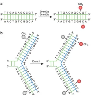
Methylation consists in the addition of a methyl group (containing one car-bon atom car-bonded to three hydrogen atoms -CH3): in the DNA of vertebrates it typically occurs at CpG sites (cytosine-phosphate-guanine sites, that is, where a cytosine is directly followed by a guanine in the DNA sequence). This pro-cess results in the conversion of the cytosine to 5-methylcytosine (see Figure 1.12). Methylated C residues spontaneously deaminate to form T residues over time; hence CpG dinucleotides steadily deaminate to TpG dinucleotides, which is evidenced by the under-representation of CpG dinucleotides in the human genome[12]. The remaining CpG sites are spread out across the genome where they are heavily methylated with the exception of CpG islands (stretches of DNA that have a higher CpG density than the rest of the genome, and will be described in detail in the next section).

DNA methylation is catalyzed by a family of DNA methyltransferases (Dn-mts), which share a similar structure with a large N-terminal regulatory domain and a C-terminal catalytic domain, but have unique functions and expression patterns. Dnmt3a and Dnmt3b can establish a new methylation pattern to unmodified DNA and are thus known as “de novo” Dnmt; on the other hand Dnmt1 functions during DNA replication to copy the DNA methylation pat-tern from the parental DNA strand onto the newly synthesized daughter strand (see Figure 1.13). Additionally, Dnmt1 also has the ability to repair DNA methylation[30]. For these reasons, Dnmt1 is called the “maintenance” Dnmt because it maintains the original pattern of DNA methylation in a cell lineage: without it, the replication machinery would produce daughter strands that are unmethylated and, over time, this would lead to passive demethylation.

DNA methylation and gene regulation

DNA methylation is a major epigenetic factor influencing gene activities, and it can repress transcription both directly and indirectly. In the first case, it can physically impede the binding of transcription factors to the gene, whereas in the second methylated DNA may be bound by methyl-CpG-binding domain pro-teins which recruit additional propro-teins that modify histones forming compact, inactive heterochromatin. In addition to this, DNA methylation also cooperates

(25)

1.5. CPG ISLANDS 19

Figure 1.12: Conversion of cytosine in 5-methylcytosine.

with histone modifications to impose a repressive state on a gene region.

Due of its vital role in gene regulation, a correctly established DNA methy-lation is essential for the normal development and functioning of organisms, and an increasing number of diseases have been found to be associated with aberrant methylation patterns: among these, cancer is one of the most studies one. The first evidence of a link between DNA methylation and cancer was demonstrated in 1983, when it was shown that the genomes of cancer cells are hypomethylated relative to their normal counterparts[16]. Tumor cells, in fact, are characterized by a loss of methylation in the repetitive regions of the genome, which causes genomic instability. In addition to this genome-wide demethyla-tion, gene-specific hypermethylation events are also observed in cancer: these typically occur at CpG islands, most of which are not methylated in normal somatic cells, and result in a silenced transcription (see Figure 1.14). For exam-ple, genes involved in cell-cycle regulation, tumour cell invasion, DNA repair, chromatin remodelling, cell signalling, transcription and apoptosis are known to become aberrantly hypermethylated and thus silenced in nearly every tumour type (see [37], supplementary information S2 and S3).

1.5 CpG islands

In the previous section, we have seen the relevance of CpG sites as methyla-tion targets. We have also introduced the concept of CpG islands as CpG-rich stretches of DNA which are usually unmethylated and can become methylated in diseases such as cancer. We will now discuss the biological importance of CpG islands in more detail and review possible definitions of CpG islands that have been proposed in literature, as well as the corresponding problematics.

(26)

Figure 1.13: Dnmt3a and Dnmt3b are the de novo Dnmts and transfer methyl groups (red) onto naked DNA. (b) Dnmt1 is the maintenance Dnmt: when DNA undergoes semiconservative replication, the parental DNA stand retains the original DNA methylation pattern (gray). Dnmt1 associates at the replication foci and precisely replicates the original DNA methylation pattern by adding methyl groups (red) onto the newly formed daughter strand (blue). Figure from [29].

Biological relevance of CpG islands

Interest in CGIs first grew in the 1980s when it was demonstrated that, in vertebrates, they are enriched in regions of the genome involved in gene tran-scription referred to as “promoters”[10]. Saxonov and others[40] found in 2005 that promoters could be classified in two classes according to their CpG con-tent: 72% of promoters belong to the class with high CpG content, and 28% are in the class whose CpG content is characteristic of the overall genome (low CpG content). In addition to this, CGIs have been shown to colocalize with the promoters of all constitutively expressed genes and approximately 40% of those displaying a tissue restricted expression profile[26].

As far as the methylation status of CpG islands is concerned, we have already discusses altered DNA methylation of CGIs (which are usually unmethylated) in development and cancer (see ref[17]). A study of CGI methylation on chromo-some 21 by Yamada and others[46] found that although most CGIs (103 out of 149) escape methylation, a sizable fraction (31 out of 149) are fully methylated

(27)

1.5. CPG ISLANDS 21

Figure 1.14: The diagram shows a representative region of DNA in a normal cell. The region shown contains repeat-rich, hypermethylated heterochromatin and an actively transcribed tumour suppressor gene (TSG) associated with a hypomethylated CpG island (indicated in red). In tumour cells, repeat-rich heterochromatin becomes hypomethylated, contributing to genomic instability. De novo methylation of CpG islands also occurs in cancer cells, resulting in the transcriptional silencing of growth-regulatory genes. Figure from [37].

even in normal peripheral blood cells. This result may however have been influ-enced by the low specificity of the CGI definition employed (as will be discussed later).

From the above considerations it is evident that knowledge of CpG islands locations plays an important role both in promoter prediction and for the iden-tification of candidate regions for aberrant DNA methylation.

Main definitions and problematics

The first formal definition of a CpG islands was given by Gardner-Gardiner and Frommer in 1987[18], as a region of at least 200 bp with the proportion of Gs or Cs, referred to as “GC content”, greater than 50%, and observed to expected CpG ratio (O/E) greater than 0.6. This ratio is computed by dividing the proportion of CpG dinucleotides in the region by what is expected by chance, when bases are assumed to be independent outcomes of a multinomial distribution:

O/E = #CpG/N

(28)

where N is the number of base pairs in the segment under consideration. Based on this definition, multiple algorithms for CpG islands identification have been developed, sometimes employing different parameter values. For example, Takai and Jones[42] considered slightly different cutoffs: a minimum length of 500 bp, a minimum GC content of 55% and a minimum O/E of 0.65. With these parameters they were able to exclude most repetitive Alu elements from the CpG island list, which otherwise required to be filtered out in the pre-processing of data, as many of them tend to be mistaken for CpG islands due to their base composition. In general, definition-based methods such these lack specificity and robustness, as an arbitrary variation of parameters can give a substantially different list of CpG islands.

The “CG cluster” algorithm described by Glass and others[20] extracts over-lapping sequence fragments containing a fixed number of CGs and having vari-able length. The histogram of these lengths shows a bimodal distribution and it is possible to select a cutoff and find regions associated with the first mode (CG clusters, or CpG islands). The distance-based “CpGcluster” algorithm by Hackenberg and others looks for clusters of CG dinucleotides according to their distance compared to a threshold distance (the median of the distance distri-bution is often employed as a reference). A p-value is then associated to each cluster according to a randomization test on the DNA sequence or by means of a theoretical probability function.

A different method was proposed by Bock and others[11]: it combines an ini-tial, sequence-based mapping of CpG islands with subsequent prediction of CpG island strengths, calculated as a combination of epigenome prediction and which express their tendency to exhibit an unmethylated, open, and transcriptionally competent chromatin structure. Lastly, Irizarry and others[24] developed an al-gorithm for CpG annotation based on Hidden Markov Models: their work was motivated by recent high-throughput measurement of epigenetic events such as differentially methylated regions (DMRs), which showed that many are DMRs not associated with CGIs but that are nevertheless in the shores of CpG-enriched sequences[23]. Therefore they developed an HMM-based approach for a more flexible definition of CpG islands which would include these newly discovered regions, based on the assumption that the property that defines a CGI is not the CpG density per se but the CpG density conditioned on GC content. In this framework, the CGI and baseline regions are the hidden states and the CpG counts are the observations that depend on these states, and CpG counts are

(29)

1.5. CPG ISLANDS 23 modeled in small intervals. Thus, the genome is divided into non overlapping segments of length s and the posterior probability of being a CGI state is esti-mated for each segment, after fitting of the model. The authors found that the CGI list, created with their method, covered 94% of the DMRs reported in [23], in comparison with the 65% covered by the GenomeBrowser CGI.

The two tracks providing mapping of CpG islands currently available on the Genome Browser are based respectively on the method of Bock and on the HMM-based algorithm of Irizarry. The main characteristics of these two differ-ent CpG islands annotations are listed in Table 1.2.

Measure CGI Genome Browser CGI HMM-based

Total CGI n° 28.691 65.535

Total CGI length 21.842.742 39.958.086

Min length 201 18

Max length 45.712 44.214

Mean length 761,3 609,7

Median length 559 408

Mean O/E ratio 0,862 0,747

(30)

(31)

CHAPTER

2

Sequence analysis methods

In this chapter we illustrate the main methods employed in this thesis. In the first section we describe different types of random reference models used in this work, both for genomic sequences and distance distributions. In the second section we introduce the details of our distance-based analysis, used to compare inter-dinucleotide distance distributions across the whole human genome. The final section is devoted to the description of a random walk representation of DNA sequences.

2.1 Random reference models

When working with statistical analyses on genomic sequences it is essential to compare the results obtained with an appropriate null model: in this way, in fact, it is possible to reject the hypothesis that the features observed could also happen by chance, and thus confirm that they are biologically significant. In our case this translates into the generation of “synthetic” DNA sequences, in which the nucleotides are picked in a random fashion following different rules. We will see that it is also possible to model the distance distributions in the random case directly, though this is derived from a sequence null model as well.

(32)

DNA sequence random models

A suitable model for the generation of random DNA sequences is necessary in any study involving the human genome: in fact, any finding has to be com-pared and validated with what would be observed if the sequence were to be randomly generated. Naturally, many possible definitions of a “random” se-quence and different models (from the naive to the more refined ones) exist: it is therefore necessary to carefully consider the best method for each study, taking into account the tradeoff between complexity and plausibility. One of the most widely used random model for DNA sequences is based on Markov chains.

A sequence {Xn} of discrete random variables is called a Markov chain if it

satisfies the Markov property: for all n ≥ 1 and (x1, x2, ...xn):

P (Xn+1= xn+1|X1= x1, ..., Xn = xn) = P (Xn+1= xn+1|Xn= xn)

That is, the conditional probability at step n + 1, given the value Xn at step

n, is uniquely determined and is not affected by any knowledge of the values at earlier times. A Markov chain is defined by:

• S = { possible xn, ∀n}: the state space;

• X0: the initial state;

• P (Xn+1= j|Xn= i), i, j ∈ S: the transition probabilities.

If for all n and i, j ∈ S, P (Xn+1= j|Xn = i) = pij independently of n, the

chain is said to be homogeneous, and we have a transition probability matrix:

      p11 p12 . . . p1m p21 p22 . . . p2m .. . ... ... ... pm1 pm2 . . . pmm       where m = |S|.

The transition probabilities determine entirely the behavior of the chain: their knowledge, together with the initial state, is sufficient to generate the whole sequence. This concept can be generalised to a m − th order Markov chain, where the state at step/time n depends on the states at the m preceding steps and not on any of the other states.

(33)

2.1. RANDOM REFERENCE MODELS 27 Markov chain models have been widely employed in the context of genomic sequences analysis as they can capture short-range correlations among bases, however it should be noted that these are still very simple models that cannot reproduce many complexities of DNA sequences, such as long-range correlations. A pictorial representation of a DNA (first-order) Markov chain is depicted in Figure 2.1: the state space consists of the four nucleotides, and the arrows rep-resent the transition probabilities from one state to the other (i.e. from A to A itself and to the other three nucleotides, and so on).

Figure 2.1: Example of a DNA Markov chain. Figure from [14]

The two types of random sequence models employed in this work are:

• Zeroth order Markov chain or Bernoulli model: this is the simplest possible model, in which the sequence is constructed by picking one of the four letters A, C, G, T with a fixed probability, independent from the preceding values. The nucleotide probabilities are determined according to the relative frequencies of the bases in the DNA sequence.

• First order Markov chain model: in this model the synthetic DNA sequence is generated taking into account the first order transition prob-abilities (namely the probability to pick a nucleotide X when we picked Y in the previous step). The entries of the transition matrix can be de-rived from the relative frequencies of nucleotides and dinucleotides in the sequence.

(34)

The transition matrix for a first order Markov chain DNA model is:       A C G T

A p(A|A) p(C|A) p(G|A) p(T |A) C p(A|C) p(C|C) p(G|C) p(T |C) G p(A|G) p(C|G) p(G|G) p(T |G) T p(A|T ) p(C|T ) p(G|T ) p(T |T )      

The transition probabilities are estimated from the biological sequence as follows: the probability p(C|A) of “picking” a C when we picked an A in the previous step is approximated by the ratio of the observed frequencies of CA dinucleotides and A nucleotides in the DNA sequence:

p(C|A) = #CA/#dinucleotides #A/#nucleotides

As an example, the transition probabilities estimated for chromosome 1 are listed below:       A C G T A 0.3265 0.1726 0.2449 0.2560 C 0.3484 0.2610 0.0486 0.3420 G 0.2864 0.2116 0.2608 0.2411 T 0.2179 0.2053 0.2499 0.3269      

Higher-order models would give rise to sequences that are more “biologi-cally” correct: for example in a second order model we would have transition probabilities such as p(A|AT ), and this “memory” could allow the reproduction of three-letter words in DNA, which correspond to codons (pieces of sequence that specify a single amino acid). However, for the present interest a first order model is sufficient, as we wish to compare our results with a reference sequence which is characterised by a similar dinucleotide bias, but with randomly dis-tributed dinucleotides across the sequence.

(35)

2.2. INTER-DINUCLEOTIDE DISTANCE ANALYSIS 29 Random model for the distance distribution

It is also possible to model the distance distribution in the random case directly: in fact, if CpGs were distributed totally at random along the chro-mosome sequence, the distances between neighboring CpG dinucleotides should follow the geometric distribution (depicted in Figure 2.2):

fx(k) = px(1 − px)k−1

Where px is the probability of x in the sequence, estimated from its frequency

in the biological sequence (i.e. pCG). The mean and variance of the distribution

are equal to: E[k] =1_q, var(k) = 1−q_q2 .

We can easily understand why this is the case, if we reckon that the geo-metric distribution is used to model the probability that the kth trial (out of k trials) is the first success, given that the success probability in a single trial is p. In this work we employ the geometric distribution as a random reference for the inter-dinucleotide distance distributions, and it proves to be very convenient as we can directly compare them without having to generate a whole synthetic sequence (which can be extremely computationally intensive).

Note that this model is not independent from the previously introduced random sequence models: the geometric distribution for inter-dinucleotide dis-tances, in fact, can be derived from a random sequence in which we pick din-ucleotides with a fixed probability, estimated from dinucleotide frequencies in the real DNA sequence. This corresponds to a zeroth order Markov model in which, instead of picking nucleotides, the sequence is constructed by picking dinucleotides.

2.2 Inter-dinucleotide distance analysis

In this section we describe a distance-based approach for the characterisation of dinucleotides distribution inside the human genome. Note that this method could also be formulated in the context of dynamical systems in terms of “return times” or “Poincar´e recurrences” of symbolic trajectories.

The outline of the method is the following: the sequence of interest is read and all the inter-dinucleotide distances are computed for the 16 different din-ucleotides as shown in Figure 3.1. We do not divide the sequence rigidly in

(36)

Figure 2.2: Example of geometric distribution for different parameters value.

dinucleotides as done in other works (see for example [8]) but, starting from the first nucleotide in the sequence, we look for every occurrence of the dinu-cleotide of interest and store the corresponding distances, which are computed in nucleotide units. These two methods are compared in Figure 3.2: notice how dividing the sequence rigidly into dinucleotides introduces the problem of having two different frames of reference, which as shown detect different CpG couples. This could pose a problem when dealing with CpG islands, because one reading frame may miss on CpG islands that are found in the second one: this is our main motivation for using a different method.

In addition to this we decided to employ a non-overlapping approach: namely, AAAA is evaluated as two AA dinucleotides with a distance of two (however, notice that this difference is irrelevant when focusing on CpGs), and all dis-tances are subtracted by one at the end of the process in order to obtain a minimum distance of 1. In this way, all dinucleotides have a minimum distance of one (using an overlapping approach would give rise to a minimum distance of zero for “double” dinucleotides only).

(37)

2.2. INTER-DINUCLEOTIDE DISTANCE ANALYSIS 31

Figure 2.3: Example of inter-dinucleotide distance computation for CG dinucleotides: the start point is indicated and C nucleotides in a CpG couple are highlighted for clarity. The distances are counted in single nu-cleotides units, and will later be subtracted by one to obtain a minimum distance of 1 for adjacent couples.

Figure 2.4: Comparison of two methods for dinucleotide analysis in the sequence: in the first case it is divided rigidly in dinucleotides, obtaining two reading frames which are not equivalent (pictures a and b). In the second case distances are computed in single nucleotides, so there are no issues with different reading frames (picture c).

In order to quantitatively compare the distributions obtained for different dinucleotides, we employ the Kullback-Leibler divergence (also known as relative entropy): this is a measure of the difference between two probability distribu-tions f (x) and g(x). It represents the information lost when g(x) is used to approximate f (x): more precisely it measures the number of additional bits required when encoding a random variable with a distribution f (x) using the alternative distribution g(x). For two probability distributions f (x) and g(x) and a random variable X, the KL divergence is defined as:

D(f ||g) = X

x∈X

f (x)logf (x) g(x)

(38)

The KL divergence has the following properties: • D(f||g) > 0;

• D(f||g) 6= D(g||f): this measure is therefore asymmetric; • D(f||g) = 0 iff f(x) = g(x) for all x ∈ X.

Considerations on the treatment of N nucleotides

When working with the Human Genome assembly, an observation which could at first come as a surprise to non-biologists is the presence of a fifth letter (besides the usual A, C, G and T) in the sequence: N. This letter stands for “aNy” base - an unknown nucleotide which could not be correctly classified: Ns are often found clustered together in areas corresponding to repetitive elements, the centromere, or other non coding regions. In most works these parts are discarded without any further consideration, but here it was found appropriate to perform an initial analysis in order to evaluate the distribution and abundance of these interspersed sequences and, most importantly for our application, the effect of their presence on the evaluation of inter-nucleotide distances. To this end, three different approaches for computing inter-dinucleotides distances in presence of Ns are compared. While looping on the DNA sequence looking for specific occurrences in order to calculate their distances, if a N is encountered three different actions are possible:

• the counting continues as if a typical nucleotide was encountered, • the distance counter is not updated: this is effectively the same as

remov-ing the Ns from the sequence,

• the distance is calculated in the standard way but then it is discarded from the distribution.

The approaches described above are more easily compared using an exam-ple: take for instance the following DNA sequence sample, for which we want to compute the distances between CpG occurrences.

AT CGAAN N N CGT T AT CG

Using the first method we would get the distance values (taken from the C to the next C) d1= (7, 6); with the second method (removing the Ns) the distances

(39)

2.2. INTER-DINUCLEOTIDE DISTANCE ANALYSIS 33 The method described above was applied to the CpG dinucleotide in the different chromosomes: the most interesting finding in this initial analysis is the fact that only a very little number of distances are discarded in method 3 due to the presence of Ns, and this number is also not directly proportional to N content in the chromosome (see Table 2.1). This unique feature is probably due to the fact that Ns are usually present in blocks, so they affect only a few distance counts, and in some chromosomes with high N content these are distributed mostly at the start and end points of the chromosome: a perfect example is chromosome 14, which has a high N content but thanks to their distribution in the sequence there is no effect on the dinucleotide distances computed. Due to all the above consideration it is therefore found here that the effect of discarding the Ns is actually negligible, and this will be the starting point for the following analyses.

(40)

Chromosome N content (%) ∆ num dist 1 9.6 37 2 2.1 20 3 1.6 5 4 1.8 10 5 1.8 5 6 2.2 9 7 2.4 15 8 2.4 7 9 14.9 38 10 3.1 22 11 2.9 7 12 2.5 11 13 17.0 4 14 17.8 0 15 20.3 9 16 12.7 4 17 4.2 7 18 4.4 9 19 5.6 4 20 5.6 5 21 27.1 14 22 32.0 9 X 2.69 21 Y 56.79 16

Table 2.1: N content for all chromosomes and corresponding dif-ference in the number of CG distances computed with methods 2 and 3.

(41)

2.3. DNA WALK 35

2.3 DNA walk

We review here different methods based on the representation of DNA se-quences as random walks, and introduce the specific conversion of the sequence into a walk employed in this thesis.

One of first works to introduce a mapping of the nucleotide sequence into a walk, termed “DNA walk”, is the one by Peng, Buildyrev and others on long range correlations in genomic sequences [32]. They define a DNA walk based on a conventional one dimensional random walk, in which a walker movers either up (u(i) = +1) or down (u(i) = −1) one unit length (u) for each step i of the walk. The net displacement (y) of the walker after l steps is the sum of the unit steps u(i) for each step i:

y(l) =

l

X

i=1

u(i)

In the case of the DNA walk, the walker steps up when a pyrimidine (C or T nucleotide) occurs along the DNA chain and down when a purine is encountered (A or G nucleotide). Two examples of the walks obtained with this method are shown in Figure 2.5. An analysis of the root mean square fluctuation about the average of the displacement, which is related to the auto correlation of the sequence, emphasised the presence of long-range correlation in nucleotide sequences, especially intron-containing genes. Furthermore, they reported a quantitative scaling of the correlation in the power law form, observed in nu-merous phenomena having a self-similar or fractal origin.

Different methods for the conversion of a nucleotide sequence into a one dimensional walk are possible, and some are reviewed in [9] (for example we could distinguish between nucleotides with strong vs weak hydrogen bonding -C and G vs T and A). Higher dimensional and more complex walks are also possible: for example in [9] nucleotides are mapped into the four cardinal points (+1, −1, +j, −j) of the complex plane, which correspond respectively to the presence of A, G, T and C nucleotides in the sequence. In this representation purines are limited to values on the real axis, while pyrimidines are restricted to the imaginary axis. An example of such a walk, computed for a noncoding region of the Helicobacter pylori bateria sequence, is shown in Figure 2.6. The authors emphasise how this walk can help locating periodicities and nucleotide structures, and they also incorporate Gaussian-based wavelet analysis to distin-guish between high and low complexity regions in genomic sequences.

(42)

Figure 2.5: DNA walk representations of (a) intron-rich human β-cardiac myosin heavy chain gene sequence and (b) the intron-less bacte-riophage λ DNA sequence. Heavy bars correspond to the coding regions of the gene. Image from [33].

In this work, we employ yet a different conversion of the nucleotide sequence into a DNA walk. Our interest here is mostly focused on dinucleotides, therefore our “walker” will:

• go up when the dinucleotide of interest is encountered (i.e. CpG); • go down otherwise.

This method provides another possible one-dimensional walk representation of the DNA sequence under analysis.

(43)

2.3. DNA WALK 37

Figure 2.6: Complex DNA walk. This graphical representation high-lights the nucleotide evolution of the DNA sequence and exposes trends in nucleotide composition. From this graphical representation, we can identify a region with an interesting nucleotide staircase structure oc-curring near bp 5150–5290. Image from [9].

(44)

(45)

CHAPTER

3

Characterisation of dinucleotide statistics

In this chapter we present the results of our genome-wide analysis of dinu-cleotide statistics. In the first section we focus on the abundance of the different dinucleotides in human DNA and compare it with the one observed for two dif-ferent types of randomly generated sequences. The second section is devoted to the inter-dinucleotide distances distributions (as obtained with the method described in Chapter 2), which are characterised and compared with the corre-sponding random models (mainly the geometric distribution).

3.1 Relative frequencies of dinucleotides

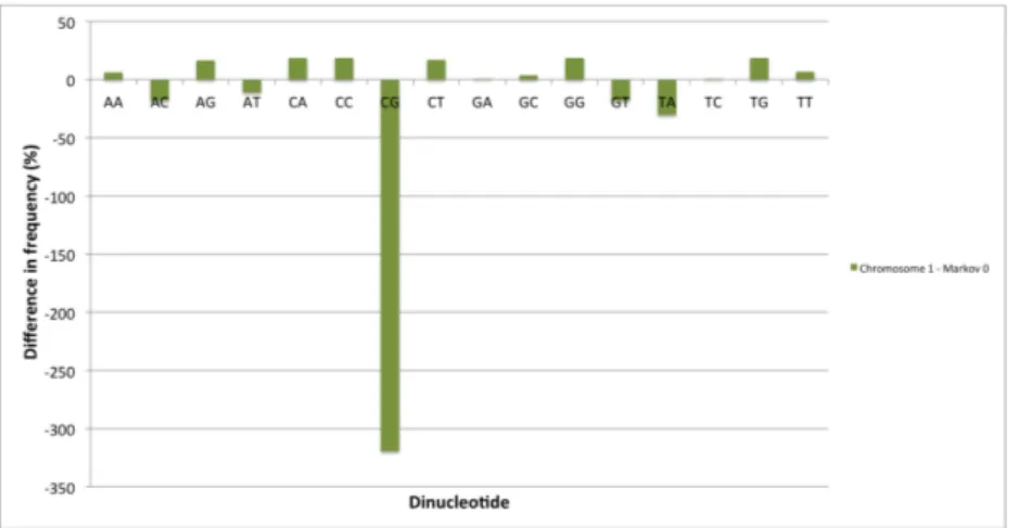
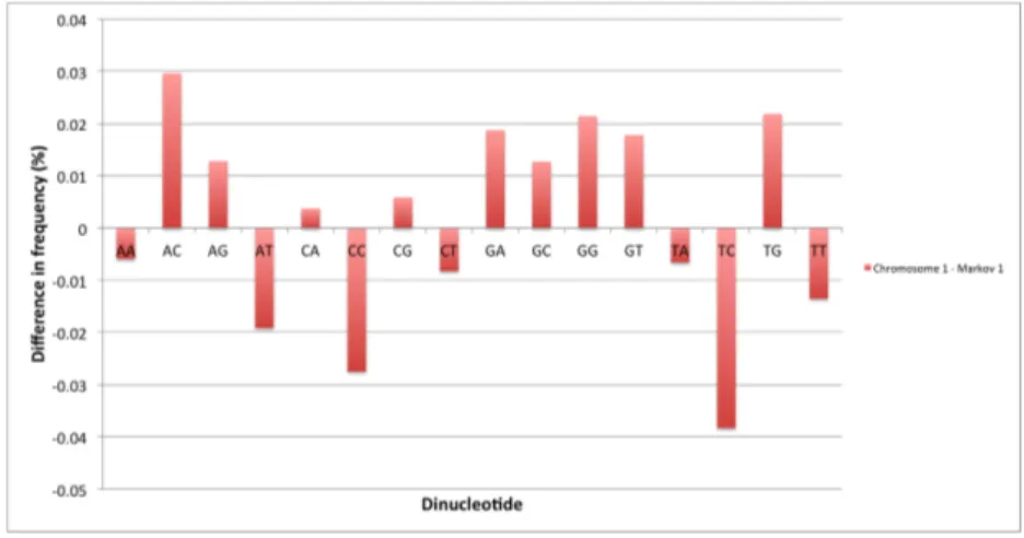
In this section we analyze the different dinucleotides abundances in the hu-man genome and compare them with the results obtained in the case of a random sequence. We consider two random sequences, generated respectively using a zeroth-order and a first-oder Markov chain (see the Methods chapter for de-tails). In Table 3.1, the relative frequencies of the 16 dinucleotides are listed for chromosome 1 (taken here as an example) and for two synthetic random sequences. The data are also plotted in Figures 3.1 and 3.3 where they can be easily inspected visually. In Table 3.2 and Figures 3.2 and 3.4 we report the percentage differences in dinucleotide abundance between the chromosome 1 sequence and the two different random sequences.

(46)

By comparing the relative frequencies values for the different dinucleotides we immediately notice that CpGs are strongly depleted in the human genome, as expected due to the methylation and mutation processes that act on the cy-tosines in the couple. It is interesting to compare the two random models: the zeroth-order Markov model does reproduce a few dinucleotides in the abundance observed in the real sequence, but the predicted amount of CpGs is much higher than the observed one. The first-oder model, which takes into account the tran-sition probability from a cytosine to a thymine, has the capability to reproduce this feature much better, as can be seen in Figure 3.3 and 3.4. Overall, the first-order Markov chain model generates sequences with a dinucleotide content extremely similar to the biological sequence: for this reason we believe that this model is appropriate for our analysis, as we wish to compare our results with sequences that contain approximately the same amount of dinucleotides, but where these are distributed randomly.

Dinucleotide Rel freq observed Rel freq Markov 0 Rel freq Markov 1

AA 0.095045182 0.069341454 0.095050808 AC 0.050228217 0.06418978 0.050213334 AG 0.07127676 0.06420494 0.071267626 AT 0.074513048 0.089614639 0.074527307 CA 0.072725744 0.064205948 0.07272302 CC 0.054485162 0.038075984 0.054500134 CG 0.010140554 0.046002714 0.010139958 CT 0.071385504 0.064255427 0.07139137 GA 0.059773523 0.064185349 0.059762304 GC 0.044171326 0.046032733 0.044165721 GG 0.054439241 0.038058532 0.054427571 GT 0.050318136 0.064241298 0.050309188 TA 0.063518745 0.089618062 0.063522939 TC 0.05985238 0.064241575 0.059875297 TG 0.07284555 0.064251727 0.072829629 TT 0.095280928 0.069479837 0.095293794

Table 3.1: Comparison of the relative frequencies of the 16 dinu-cleotides in the Chromosome 1 sequence and in two different ref-erence random sequences (generated by a zeroth and first order Markov chain model).

(47)

3.1. RELATIVE FREQUENCIES OF DINUCLEOTIDES 41

Dinucleotide Percentage difference Markov 0 Percentage difference Markov 1

AA 6.4162 -0.0059 AC -18.1161 0.0296 AG 16.7448 0.0128 AT -11.1572 -0.0191 CA 18.4022 0.0037 CC 18.5459 -0.0275 CG -319.2884 0.0059 CT 16.8062 -0.0082 GA 0.7528 0.0188 GC 3.6798 0.0127 GG 18.5344 0.0214 GT -17.9997 0.0178 TA -30.4021 -0.0066 TC 0.7968 -0.0383 TG 18.4784 0.0219 TT 6.4407 -0.0135

Table 3.2: Comparison of the percentage differences in dinucleotide frequencies between the Chromosome 1 sequence and two different reference random sequences (generated by a zeroth and first order Markov chain model).

Figure 3.1: Comparison of relative frequencies of dinucleotides in chro-mosome 1 and in a random sequence generated with a zeroth-order Markov chain.

(48)

Figure 3.2: Percentage difference in dinucleotide content between the chromosome 1 sequence and a random sequence generated with a zeroth-order Markov chain.

Figure 3.3: Comparison of relative frequencies of dinucleotides in chro-mosome 1 and in a random sequence generated with a first-order Markov chain.

(49)

3.1. RELATIVE FREQUENCIES OF DINUCLEOTIDES 43

Figure 3.4: Percentage difference in dinucleotide content between the chromosome 1 sequence and a random sequence generated with a first-order Markov chain.

(50)

3.2 Comparison of dinucleotide distance

distri-butions

In this section, we present and describe the results of our distance-based characterisation of dinucleotide positioning in the human genome. The distance distributions for the different dinucleotides are first compared with each other and then with the random models.

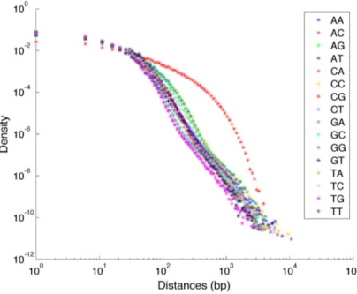
The histogram of the inter-dinucleotide distances for the CpGs is highly pos-itive skewed and it spans a wide range of length values. The overall shape of the distance distribution for the other dinucleotides is quite similar to this one, so we choose to employ log-log plots that enable a better analysis of the distri-butions behaviour in the tails. In Figure 3.5 the distance histograms for all 16 dinucleotides are plotted on a log-log scale. In order to reduce noise in the tails of the plots, partial logarithmic binning was applied for distances over a fixed threshold, substantially improving the quality and readability of the plots.

We can see in this figure that the red curve, corresponding to CpG dinu-cleotides, clearly stands out from the other 15 curves, corresponding to the re-maining dinucleotides. In order to quantitatively characterise the distributions we report in Table 3.3 some descriptive values for the different dinucleotides. All distances values throughout this work are intended in bp (base pairs). Com-parison of the mean and median values for the different dinucleotides shows that both of them are significantly higher for CpGs: this fact, combined with the inspection of the log log plots in Figure 3.5 indicates that the CpG distance distribution has heavier tails when compared to the other dinucleotides.

(51)

3.2. COMPARISON OF DINUCLEOTIDE DISTANCE DISTRIBUTIONS 45

Figure 3.5: Histograms of the inter-dinucleotide distances distributions for all dinucleotides in log log scale.

Dinucleotide Max distance Mean distance Median distance

AA 5874 13.24 7 AC 4039 18.86 12 AG 4238 13.30 8 AT 4154 11.94 7 CA 3427 12.79 9 CC 10266 23.11 13 CG 4210 100.40 41 CT 6245 13.29 8 GA 4611 15.85 10 GC 3274 22.44 13 GG 5256 23.10 13 GT 5763 18.82 12 TA 4743 14.23 8 TC 6172 15.85 10 TG 3562 12.76 9 TT 11516 13.20 7

(52)

AA AC AG AT CA CC CG CT GA GC GG GT TA TC TG TT AA 0.113 0.052 0.052 0.070 0.172 0.994 0.052 0.043 0.441 0.172 0.112 0.036 0.043 0.070 0.000 AC 0.113 0.098 0.168 0.125 0.047 0.678 0.099 0.030 0.139 0.046 0.000 0.094 0.03 0.126 0.114 AG 0.044 0.090 0.018 0.009 0.133 0.950 0.000 0.028 0.230 0.134 0.089 0.014 0.028 0.009 0.044 AT 0.046 0.145 0.017 0.017 0.189 1.046 0.017 0.057 0.304 0.190 0.143 0.019 0.057 0.017 0.046 CA 0.058 0.101 0.009 0.017 0.161 0.985 0.009 0.041 0.235 0.163 0.100 0.024 0.041 0.000 0.058 CC 0.193 0.058 0.205 0.276 0.275 0.539 0.205 0.097 0.094 0.006 0.059 0.142 0.097 0.277 0.195 CG 2.288 2.095 2.750 2.741 3.237 1.226 2.745 2.246 1.459 1.225 2.098 1.998 2.254 3.224 2.292 CT 0.044 0.090 0.000 0.018 0.009 0.133 0.951 0.028 0.231 0.134 0.089 0.014 0.028 0.009 0.044 GA 0.041 0.030 0.030 0.066 0.049 0.072 0.800 0.030 0.201 0.075 0.029 0.029 0.000 0.050 0.042 GC 0.285 0.099 0.232 0.310 0.279 0.071 0.603 0.233 0.149 0.075 0.099 0.193 0.149 0.281 0.288 GG 0.192 0.058 0.206 0.275 0.276 0.006 0.541 0.206 0.100 0.098 0.058 0.142 0.100 0.278 0.193 GT 0.112 0.000 0.097 0.166 0.124 0.047 0.679 0.098 0.030 0.139 0.046 0.093 0.030 0.125 0.113 TA 0.033 0.089 0.019 0.024 0.035 0.116 0.908 0.019 0.028 0.238 0.118 0.088 0.028 0.035 0.033 TC 0.041 0.030 0.030 0.066 0.049 0.072 0.801 0.030 0.000 0.202 0.075 0.029 0.029 0.050 0.042 TG 0.058 0.102 0.009 0.017 0.000 0.162 0.987 0.009 0.041 0.236 0.164 0.101 0.024 0.041 0.058 TT 0.000 0.114 0.053 0.052 0.070 0.174 0.996 0.053 0.044 0.444 0.173 0.113 0.037 0.044 0.070

Table 3.4: Kullback-Leibler divergence of dinucleotide distance dis-tributions.

Figure 3.6: Heatmap of the KL-divergence of dinucleotide distance distributions.

(53)

3.2. COMPARISON OF DINUCLEOTIDE DISTANCE DISTRIBUTIONS 47 Comparison with the random models

In the Methods chapter we introduced two different models for the gener-ation of random references sequences, and we also described how the distance distribution in the random case can be modelled as a geometric distribution.

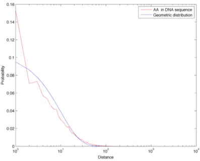
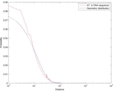
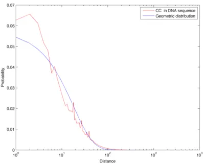
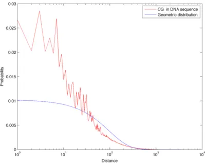
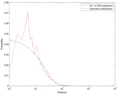
In Figure 3.14 we compare the distance frequencies for CpGs in the DNA sequence of chromosome 1 with all three references: first of all it is possible to notice how the green curve (Markov 0 chain sequence) is greatly enriched in short distances. This is due to the fact that CpG abundance in this random sequence is much greater than in the real biological sequence, as described in Section 3.1. Furthermore, this model also completely fails in describing the tails found in the real distance distribution: for these reason, we discard the Markov 0 sequence as a good random reference for the distance distributions. On the other hand, the geometric and Markov 1 curves correspond quite well and they both reflect the properties of a sequence with a similar amount of dinucleotides, but which are positioned randomly. In Figures 3.8 to 3.22 we report the linear-log plots of distances distribution for the 16 dinucleotides, compared with the geometric distribution (which is much less computationally intensive to generate than the Markov 1 sequence).

Figure 3.7: Comparison of CpGs distance frequencies in chromo-some 1, in two random reference sequences (generated with a zeroth and first order Markov chain) and in the geometric distribution for CpGs.