UNIVERSITY OF PISA
DEPARTMENT OF ELECTRICAL SYSTEMS AND AUTOMATION
OBSTACLE AVOIDANCE FOR A GAME THEORETICALY CONTROLLED
FORMATION OF UNMANNED VEHICLES
Doctoral Thesis by
Mehmet Eren ERDOĞAN
Cycle XXII
Supervisor: Prof. Mario INNOCENTI
UNIVERSITY OF PISA
DEPARTMENT OF ELECTRICAL SYSTEMS AND AUTOMATION
OBSTACLE AVOIDANCE FOR A GAME THEORETICALY CONTROLLED
FORMATION OF UNMANNED VEHICLES
Doctoral Thesis by
Mehmet Eren ERDOĞAN
Cycle XXII
Supervisor: Prof. Mario INNOCENTI
Student: Mehmet Eren ERDOĞAN
FOREWORD
I would like to extend my sincere gratitude and appreciation to Prof. Mario Innocenti
and Prof. Lorenzo Pollini for their guidance, supports and helps.
All my past and present friends and colleagues deserve special thanks, and I must say
that it has been four years full of joy and experience thanks to them. It was a pleasure for
me to share the same ambient with them during my doctoral studies.
Acknowledgement also goes to all the department members which assisted and helped
me a lot to adapt especially during my first years in the faculty.
Also, I would like to thank a lot to my parents which always supported, and motivated
me and have been very close to me even if they were physically far away. The
completion of this thesis would not have been possible without their encouragement and
support.
Finally, my very special, endless and immeasurable thanks go to my wife and little son.
My little son has always been a motivation factor for me. I am forever grateful for my
wife steadfast encouragement, love, and willingness to endure many sacrifices, to enable
me to pursue this thesis, which without her support I would not have had the confidence
to finish.
This thesis is dedicated to my beloved wife and son.
TABLE OF CONTENTS
Page
TABLE OF CONTENTS
vi
ABBREVIATIONS
vii
LIST OF FIGURES
ix
1. INTRODUCTION
1
1.1. A Historical Survey of Robotics
4
2. PROBLEMS CONSIDERED AND MOTIVATING APPLICATIONS
7
2.1. Navigation and Obstacle Avoidance
7
2.2. Formations and Multi-Agents Robotics
7
3. LITERATURE SURVEY
10
3.1. Navigation and Obstacle Avoidance
10
3.2. Formations and Multi-Agents Robotics
11
4. BACKGROUND ON GAME THEORETICAL APPROACH
16
5. MODEL AND CONTROL
18
5.1. Robot Dynamics
18
5.2. Formation of Robots
19
5.3. Formation Cost Functions
21
5.4. Nash Equilibrium and Differential Games
23
5.5. NSB Behavioral Control
26
6. STABILITY ANALYSIS
31
6.1. Stability Analysis for Receding Horizon Nash Control
31
6.2. Stability Analysis for NSBBC Obstacle Avoidance Algorithm
32
7. SIMULATIONS
33
8. CONCLUSION
52
vii
ABBREVIATIONS
SLAM
: Simultaneous Localizations And Mapping
GPS
: Global Positioning System
NSBBC
: Null Space Based Behavioral Control
VLSR
: Very Large Scale Robotic
ix
LIST OF FIGURES
Page
Figure 1.1 : Water Raising Device of Al-Jazari...
4
Figure 1.2 : Elektro, the Westinghouse Motoman. ...
5
Figure 1.3 : Honda’s Asimo Serving Coffee... 6
Figure 5.1 : Triangular Formation of Robots...
19
Figure 5.2 : A Formation of 4 Robots and Related Incidence Matrix. ...
19
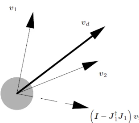
Figure 5.3 :
A case of two simultaneous behaviors: is the output of an obstacle
v1avoidance task while
v2is the output of a trajectory tracking task. ... 27
Figure 5.4 :
Sketch of the null-space-based behavioral control in a 2-task example 27
Figure 7.1 : Triangle formation shape...
33
Figure 7.2 :
Phase plane of unmanned vehicles where the radius is 3 times the real
dradius of the obstacle. ... 34
Figure 7.3 :
...
X position errors of the unmanned vehicles for the simulation shown in
Fig.7.2.
.. 34
Figure 7.4 :
...
Y position errors of the unmanned vehicles for the simulation shown in
Fig.7.2.
.. 35
Figure 7.5 :
Phase plane of unmanned vehicles where the radius is equal to the
dreal radius of the obstacle ... 35
Figure 7.6 :
...
Phase plane of unmanned vehicles where all the vehicles execute
obstacle avoidance algorithm
35
Figure 7.7 :
...
X position errors of the unmanned vehicles for the simulation shown in
Fig.7.6.
.. 36
Figure 7.8 :
...
Y position errors of the unmanned vehicles for the simulation shown in
Fig.7.6.
.. 36
Figure 7.9 :
...
Phase plane of unmanned vehicles with a moving small obstacle which
moves toward the vehicles where all the vehicles execute the obstacle
avoidance algorithm
37
Figure 7.10 :
...
X position errors of the unmanned vehicles for the simulation shown in
Fig.7.9.
.. 37
Figure 7.11 :
...
Y position errors of the unmanned vehicles for the simulation shown in
Fig.7.9.
.. 38
Figure 7.12 :
...
Control signals that affect the leader vehicle for the simulations shown
in Fig.7.9
.
38
Figure 7.13 :
...
Phase plane of unmanned vehicles with a moving small obstacle which
crosses the trajectory of the vehicles where all the vehicles execute the
obstacle avoidance algorithm
39
Figure 7.14 :
...
X position errors of the unmanned vehicles for the simulation shown in
Fig.7.13.
39
Figure 7.15 :
...
Y position errors of the unmanned vehicles for the simulation shown in
x
Figure 7.16 :
...
Control signals that affect the leader vehicle for the simulations shown
in Fig.7.13
.
40
Figure 7.17:
...
Phase plane of unmanned vehicles with a moving small obstacle which
moves on the same direction with the vehicles where all the vehicles
execute the obstacle avoidance algorithm
40
Figure 7.18 :
...
X position errors of the unmanned vehicles for the simulation shown in
Fig.7.17.
41
Figure 7.19 :
...
Y position errors of the unmanned vehicles for the simulation shown in
Fig.7.17.
41
Figure 7.20 :
...
Control signals that affect the leader vehicle for the simulations shown
in Fig.7.17
.
41
Figure 7.21:
...
Phase plane of unmanned vehicles with a moving small obstacle which
moves toward the vehicles where all the vehicles execute the obstacle
avoidance algorithm and one of the vehicles slightly collides with the
obstacle
.. 42
Figure 7.22 :
...
X position errors of the unmanned vehicles for the simulation shown in
Fig.7.21.
42
Figure 7.23 :
...
Y position errors of the unmanned vehicles for the simulation shown in
Fig.7.21.
43
Figure 7.24 :
...
Control signals that affect the leader vehicle for the simulations shown
in Fig.7.21
.
43
Figure 7.25:
...
Phase plane of unmanned vehicles with a moving bigger obstacle which
moves toward the vehicles where all the vehicles execute the obstacle
avoidance algorithm
44
Figure 7.26 :
...
X position errors of the unmanned vehicles for the simulation shown in
Fig.7.25.
44
Figure 7.27 :
...
Y position errors of the unmanned vehicles for the simulation shown in
Fig.7.25.
44
Figure 7.28 :
...
Control signals that affect the leader vehicle for the simulations shown
in Fig.7.25
.
45
Figure 7.29:
...
Phase plane of unmanned vehicles with a suddenly appearing small
obstacle where all the vehicles execute the obstacle avoidance algorithm
45
Figure 7.30 :
...
X position errors of the unmanned vehicles for the simulation shown in
Fig.7.29.
46
Figure 7.31 :
...
Y position errors of the unmanned vehicles for the simulation shown in
Fig.7.29.
46
Figure 7.32 :
...
Control signals that affect the leader vehicle for the simulations shown
in Fig.7.29
.
46
Figure 7.33:
...
Phase plane of unmanned vehicles with a suddenly appearing bigger
obstacle where all the vehicles execute the obstacle avoidance algorithm
47
Figure 7.34 :
...
X position errors of the unmanned vehicles for the simulation shown in
Fig.7.33.
47
Figure 7.35 :
...
Y position errors of the unmanned vehicles for the simulation shown in
Fig.7.33.
47
Figure 7.36 :
...
Control signals that affect the leader vehicle for the simulations shown
xi
Figure 7.37:
...
Phase plane of unmanned vehicles with two immobile obstacles where
all the vehicles execute the obstacle avoidance algorithm
48
Figure 7.38 :
...
X position errors of the unmanned vehicles for the simulation shown in
Fig.7.37.
49
Figure 7.39 :
...
Y position errors of the unmanned vehicles for the simulation shown in
Fig.7.37.
49
Figure 7.40 :
...
Control signals that affect the leader vehicle for the simulations shown
in Fig.7.37
.
49
Figure 7.41:
...
Phase plane of unmanned vehicles with two successively immobile
obstacles where all the vehicles execute the obstacle avoidance
algorithm
50
Figure 7.42 :
...
X position errors of the unmanned vehicles for the simulation shown in
Fig.7.41.
51
Figure 7.43 :
...
Y position errors of the unmanned vehicles for the simulation shown in
Fig.7.41.
51
Figure 7.44 :
...
Control signals that affect the leader vehicle for the simulations shown
in Fig.7.41
.
51
1. INTRODUCTION
The word "robot" (from robota, Czech for "work") made its public debut in 1920, when it premiered on stage in Karel Čapek's play R.U.R. (Rossum's Universal Robots) [1]. The play told of a world in which humans relaxed and enjoyed life while robots - imitation humans - happily did whatever labor needed to be done. Reality has not yet reached that far, but today there are machines that have a high degree of autonomy and that can independently perform very complex tasks in which they interact with the environment and make on-line decisions. Much of the progress has taken place in the past few decades, during which the continuous development of hardware has made way for increasingly more advanced software.
Traditionally robots were thought of as humanoids, but today according to most people working in the robotics field, what defines a robot is its ability to function independently rather than its physical appearance. In 1998, Professor Ronald C. Arkin, co-worker and later director of the Mobile Robot Laboratory at Georgia Institute of Technology, made below written definition [2];
The role of autonomous robots in our lives is increasing in many fields. The robots are desired in many tasks for their high speed, precision and repeatability. The robots are also being employed in the areas which are hazardous, dangerous or boring for humans. The working areas of robots are enlarging from idealized areas, like industrial plants, to work in natural environments or to serve humans in their complicate homes. New working areas bring new problems for researchers. By the increasing demands for robots in different areas, the robots need to be more adaptive to changing or unknown environmental conditions in the workplace and they should be more intelligent to be able to make their own decisions in these conditions.
“An intelligent robot is a machine able to extract information from its environment and use knowledge about its world to move safely in a meaningful purposive manner”.
Robots can adapt to complex environments and perform tasks more intelligently by working in groups. Robot groups may be composed of many different kinds of robots like ground vehicles, aerial vehicles, underwater vehicles or spacecrafts. A robot group may be homogenous; each member in the group may be identical, or it can be heterogeneous; the group may include different kinds of robots. Using a team of simple robots is advantageous than using a single but more complicated robot in many ways. Robot’s
working in groups brings flexibility in a given task. If the robots of a group are doing a task together, the robots can learn about the environmental conditions more quickly by gathering sensor information from a variety of sensors of each member. Besides, if one of the robots gets hurt during the task, the remaining ones can accomplish the task. This makes the robot group systems more fault tolerant than single robot systems. Since using a group of robots brings the possibility of parallel processing, the time required for the completion of the task decreases, especially when it is a distributed task, like search and rescue or mapping of unknown areas.
Robot groups can coordinate in many ways. Some robot groups may execute coordination in which the robots move in a scattered manner like the bees of a beehive or the control of the robot group may require a more strict formation like the swallows. The shape formation is very important for coordination of mobile robot groups because it increases the capability of a robot group by increasing the competence and the security of the group. The shape formation is applicable in many tasks like formation flight, flocking and schooling, transportation systems, search-and-rescue operations, competitive games, reconnaissance and surveillance.
The shape formation in mobile robots is a challenging topic and there are many researches on that subject. For robot groups coordinating with shape formation, the flexibility of the shape formation is very important. With the increasing demand for autonomous robots in different fields, many different kinds of formation shapes are required. In non-idealized environments, forming many of the simple shapes may not be feasible. Besides, many different task definitions may require very complicated formation shapes. Another important issue of shape formation is the fault-tolerance. The shape formation algorithm should guarantee the completion of the task even if some of the group members are hurt. Since different tasks require different types of robot groups, a formation shape algorithm should also be flexible in the number and the heterogeneity of the team members.
Control of a robot group can be centralized or decentralized. In the centralized control, the data is collected in a central control unit and the control commands are sent from that unit to the robots. This central unit can be an independent computer or can be one of the members of the robot group which has a higher computational capacity. The central control unit receives a collection of the data from the robot group and the decision for each member is done according to this knowledge.
In the decentralized control, each member in the robot group gathers data using its own sensors and decides about its move according to its role definition in the desired task. In some cases, there are also some local communications among the group members.
In decentralized control, the members have a local sense of the group because the knowledge is limited by the sensor angle and occlusions. On the other hand, since in the centralized control all the data are collected by the central unit, the effects of the view angle limitation and the occlusions can be compensated. The central unit has an overall view of the robot group condition. This leads to a better decision. In the central control, complete solution and global optimum is more likely to be achieved.
One of the limitations of the centralized control is the communication. In the centralized control, the moves of agents in the group are decided by the central unit and these commands are sent to each agent. As the number of the agents increases, the communications load of the central unit increases. This can be seen as a bottleneck for centralized control but there are studies which solves this problem by decreasing the communication load on the central unit.
In robot coordination, the robustness of the algorithm to robot failures is very important. In centralized control, the detection of agent failure is available. In such a case, the central unit can decide for a better strategy of the robot group for the task to be executed in the best way available. On the other hand, in centralized controls, the failure of the central unit is a major problem to cause task failure.
Given the a priori knowledge of the environment and the goal position or trajectory to track, mobile robot navigation refers to the robot’s ability to safely move towards the goal using its knowledge and the sensorial information of the surrounding environment. Even though there are many different ways to approach navigation, most of them share a set of common components or blocks, among which path planning and obstacle avoidance play a key role. Given a map and a goal location, path planning involves finding a geometric path from the robot actual location to the goal. This is a global procedure whose execution performance is strongly dependent on a set of assumptions that are seldom observed in nowadays robots. In fact, in mobile robots operating in unstructured environments, or in service and companion robots, the a priori knowledge of the environment is usually absent or partial, the environment is not static, i.e., during the robot motion it can be faced with other robots, humans or pets, and execution is often associated with uncertainty. Therefore, for a collision free motion to the goal, the global path planning has to be associated with a local obstacle handling that involves obstacle detection and obstacle avoidance. Obstacle avoidance refers to the methodologies of shaping the robot’s path to overcome unexpected obstacles. The resulting motion depends on the robot actual location and on the sensor readings. There are a rich variety of algorithms for obstacle avoidance from basic re-planning to reactive changes in the control strategy. Proposed techniques differ on the use of sensorial data and on the motion control strategies to overcome obstacles.
The thesis provides a game theoretical approach to the control of a formation of unmanned vehicles. The objectives of the formation are to follow a prescribed trajectory, avoiding obstacle(s) while maintaining the geometry of the formation. Formation control is implemented using game theory while obstacles are avoided using Null Space Based Behavioral Control algorithm. Different obstacle avoidance scenarios are analyzed and compared. Numerical simulation results are presented, to validate the proposed approach.
In Chapter 2 it is given the considered problems and motivating applications. A literature review on formation control and obstacle avoidance can be found in Chapter 3. In Chapter 4 it is provided background on game theoretical approach. Chapter 5 is on the modeling and control of mobile robots. In Chapter 6 stability analysis both for receding horizon Nash control and NSBBC algorithm are made. Numerical simulations are shown in Chapter 7. Finally Chapter 8 concludes the thesis and indicates possible future directions.
1.1 A Historical Survey of Robotics
Constructing machines that can interact with the environment and even help or replace humans in performing dangerous or tedious tasks is not a new idea. Early work in automation and robotics was made by, for instance, the Arab engineer Al-Jazari (1136-1206) who, among other things, invented the earliest known automatic gates, which were driven by hydropower [3], [4]. He also invented automatic doors as part of one of
his elaborate water clocks,and designed and constructed a number of other automata,
including automatic machines and home appliances powered by water. According to Encyclopedia Britannica, the Italian Renaissance inventor Leonardo da Vinci may have been influenced by the classic automata of Al-Jazari. Later, in the 15th century,
Leonardo da Vinci made drawings for the construction of a mechanical knight [5]. In the
following centuries, many similar ideas saw the light of day, but not until the last century has technology reached the point where the realization of truly interacting machines is possible.
The American company Westinghouse Electric Corporation produced a series of human-resembling machines in the 1920’s and 30’s, some of them which could perform simple tasks such as vacuum cleaning. None of these machines were in a strict sense interacting with the environment but one of them, the humanoid "Elektro" (1939), had among his other skills (including blowing balloons and smoking cigarettes) the ability to distinguish between red and green light [6].
Figure 1.2 : Eletkro, the Westinghouse Motoman.
The first machines that could actually respond to stimuli are claimed to be Elmer and Elsie [7,8], two turtle-like machines on wheels that were developed by neurophysiologist William Grey Walter at Burden Neurological Institute, England, in 1948 - 49. Elmer and Elsie (names originating from ELectroMEchanical Robot, Light-Sensitive) had a light sensor, touch sensor, propulsion motor, steering motor, and a two vacuum tube analog computer. Even with this simple design, Grey demonstrated that his robots exhibited complex behaviors. By attaching light emitting sources on each of the two robots, they could even be made to interact with each other, something that was considered quite revolutionary at the time. Soon thereafter the first commercial industrial robots entered the market. The first models were only used to perform easy and repetitive tasks in static environments, such as for instance pick and place operations, painting, welding, etc., but over the years industrial robots have become increasingly more advanced and are now used in settings where a high degree of autonomy is required.
The rapid process in the electronics field has been the essential for the development within the field of robotics. The first robots had very simple control circuits based on electron tubes. In 1947, researchers at Bell Laboratories invented the transistor, which had the benefits of being much smaller and requiring significantly less power than the electron tube. This new device soon replaced the electron tube in most applications, but the real breakthrough for robotics came after the launch of the programmable microprocessor in the early seventies. Not only were these processors small enough to be incorporated in a freely movable body, they also made the cost for computer power drop dramatically.
There was a boost in the market for industrial and military robots after the arrival of the microprocessor. In the seventies and early eighties many companies started activities in the field of industrial robotics; among them were companies such as General Motors, General Electric, ASEA and KUKA. Several Japanese companies also joined this new trend and soon industrial robots became a common sight in manufacturing industries. However, nothing like that was seen in the market for domestic robots or entertainment robots intended for personal or small scale use. Even though public interest has always been substantial and experienced yet another top in the early eighties with the release of the Star Wars films and TV series like Star Trek, progress has been very slow in this area. Most probably the main reason for this has been the hardware cost. Prices on sensors and high precision mechanics have not decreased at the same rate as the price on computer power and are still comparatively high. Hardware prices have made it nearly impossible for companies that produce robots for private use to be commercially profitable. Besides this, another damping factor is that it has turned out to be more difficult than many anticipated to mimic the amazing ability seen in animals and humans to efficiently weed out relevant information from a potentially very large data set and to combine information to draw the "right" conclusions. In the attempts to solve these problems, a wide range of more or less independent research areas have evolved, covering disciplines such as computer vision, filtering, speech recognition and data fusion.
In recent years, the attempts to manufacture "Artificial Intelligence" have started to pay off. Today's robots are more reliable and can handle much more complex situations than their predecessors. Also, in the last years, prices on hardware have started to go down
[9]. Although many technical problems remain to be solved, robots for civil use, like
Honda’s Asimo, have started to appear in a variety of different areas. In the future we will most likely see robots in many new applications.
2. PROBLEMS CONSIDERED AND MOTIVATING
APPLICATIONS
The research problems considered in this thesis stem from two areas of robotics. Both are in the subfield called mobile robotics. The first research area is navigation and obstacle avoidance which basically deals with the question of getting from A to B in a safe and efficient manner. The second research area is multi-robot coordination. This is a somewhat broader area where the common theme is that of trying to achieve a collective goal using a group of robots, e.g. stay in a prescribed formation.
2.1 Navigation and Obstacle Avoidance
The problem of programming a mobile robot to move from one place to another is of course as old as the first mobile robot. This is, however, not as easy as one might think. Questions like “What path should be chosen to get to the goal location?” and “How fast and how close to the obstacles can the robot go without compromising safety?” need to be considered.
Obstacle avoidance refers to the methodologies of shaping the robot’s path to overcome the obstacles. The resulting motion depends on the robot actual location and on the sensor readings. There are a rich variety of algorithms for obstacle avoidance from basic re-planning to reactive changes in the control strategy. Proposed techniques differ on the use of sensorial data and on the motion control strategies to overcome obstacles.
In the literature there are various applications where it is assumed that it is given a high-quality map of the immediate surroundings of the robot. It must be noted however, that map building and localization contains a whole research field in itself. In [10], the area of simultaneous localization and mapping (SLAM) is investigated. Since GPS is not an option for indoor applications, this problem is quite hard, as can be seen by comparing a 15th century explorers map with the satellite images available today.
2.2 Formations and Multi-Agents Robotics
The thought of cooperating robots has received an increasing amount of attention in recent years. Besides the philosophical interest in cooperating machines the main reason is to try to take advantage of “strengths in numbers”, i.e., that there are properties like
Efficiency Flexibility
Redundancy/Robustness Price reduction
Feasibility
to be gained. Having several robots doing something often means that you have the flexibility of dividing the robots into groups working at different locations. Having many also implies robustness, since losing one robot leaves the others intact to finish the mission. The mobile robots of today are typically produced in small numbers; however, if there is a big increase in multi-agent applications, there might be a price reduction due to mass production benefits. Efficiency can be gained in terms of e.g. fuel consumption in formation flight. Finally, some missions are impossible to carry out with only one robot; these include deep space interferometry, a satellite imaging application, and the surveillance of large areas or buildings.
Following [2], the coordination problems can be divided into the following fields;
Foraging/Consuming, where randomly placed objects in the environment are to be
found and either carried somewhere or operated on in place. This includes collecting rocks on e.g. Mars.
Grazing, where an area should be swept by sensors or actuators. This includes lawn mowing (e.g. the Husqvarna Solar Mower) and vacuuming (e.g. the Electrolux Trilobite). Special cases of area sweeping include so-called search-and-rescue and pursuit-evasion scenarios. In these situations the looked for item, e.g. a missing person or an enemy vehicle, is moving.
Formation keeping, where the robots are to form some geometric pattern and maintain it while moving about in the world. Applications include formation flight for fuel efficiency and coordinated motion for collaborative lifting of large objects. In this area biological influences are very common and efforts are being made both to understand animal flocking/schooling and copy their effective strategies. A satellite application called deep space interferometry requires a large and exact sensor spacing which would be impossible to achieve with a single satellite.
Traffic control, where a number of vehicles share a common resource, highways or airspace, while trying to achieve their individual goals. In automated highway projects, the problem scales have ranged from keeping inter-vehicle spacing (formation keeping) via lane changes to choosing routes that minimize the overall effect of traffic jams. Air traffic control investigations, are motivated by the increasing congestion around major airports. The hope is to improve efficiency without compromising the vital safety.
The properties of flexibility and robustness is of course very attractive with the armed forces as is shown in the following quote “The U.S. military is considering the use of
multiple vehicles operating in a coordinated fashion for surveillance, logistical support, and combat, to offload the burden of dirty, dangerous, and dull missions from humans.”
Problems facing a multi-agent team operating in a limited space include blockage and collisions. More generally, a highly distributed system might generate competition rather than cooperation. Attempts to exploit such inter-robot competition in a market economic framework has been investigated in e.g. [11]. Finally there is always a cost of communication, in terms of additional hardware, increased computational load, and energy consumption. The old saying “Too many cooks spoil the broth” may explain the possible drawbacks of a multi-agent approach.
3. LITERATURE SURVEY
In this section we will take a look at examples of current research in the subfields of obstacle avoidance and formation control.
3.1 Navigation and Obstacle Avoidance
The problem of navigation and obstacle avoidance deals with making a robot move from one position to another as efficiently as possible, while not bumping into things on the way. There are a rich variety of algorithms for obstacle avoidance from basic re-planning to reactive changes in the control strategy. Proposed techniques differ on the use of sensorial data and on the motion control strategies to overcome obstacles.
The Bug’s algorithms [12], [13], follow the easiest common sense approach of moving directly towards the goal, unless an obstacle is found, in which case the obstacle is contoured until motion to goal is again possible. In these algorithms only the most recent values of sensorial data are used.
Path planning using artificial potential fields, [14], is based on a simple and powerful principle that has an embedded obstacle avoidance capability. The robot is considered as a particle that moves immersed in a potential field generated by the goal and by the obstacles present in the environment. The goal generates an attractive potential while each obstacle generates a repulsive potential. Obstacles are either a priori known, (and therefore the repulsive potential may be computed off-line) or line detected by the on-board sensors and therefore the repulsive potential is on-line evaluated. Besides the obstacle avoidance functionality, the potential field planning approach incorporates a motion control strategy that defines the velocity vector of the robot to drive it to the goal while avoiding obstacles.
The Vector Field Histogram, [15], generates a polar histogram of the space occupancy in the close vicinity of the robot. This polar histogram, which is constructed around the robot’s momentary location, is then checked to select the most suitable sector from among all polar histograms sectors with a low polar obstacle density and the steering of the robot is aligned with that direction.
Elastic bands [16] as a framework that combines the global path planning with a real-time sensor based robot control aiming at a collision free motion to the goal. An elastic
band is a deformable collision-free path. According to [16], the initial shape of the elastic band is the free path generated by a planner. Whenever an obstacle is detected, the band is deformed according to an artificial force, aiming at keeping a smooth path and simultaneously maintaining the clearance from the obstacles. The elastic deforms as changes in the environment are detected by the sensors, enabling the robot to accommodate uncertainties and to avoid unexpected and moving obstacles.
A dynamic approach to behavior-based robotics proposed in [17], [18], models the behavior of a mobile robot as a non-linear dynamic system. The direction to the goal is set as a stable equilibrium point of this system while the obstacles impose an unstable equilibria point of this non-linear dynamics. The combination of both steers the robot to the goal while avoiding obstacles.
The Null Space Based Behavioral Control (NSB Behavioral Control) strategy is based on degrading the general obstacle avoidance process into smaller problems which are less complex [19], [20]. Each task velocity is computed as if it were acting alone; then, before adding its contribution to the overall vehicle velocity, a lower-priority task is projected onto the null space of the immediately higher-priority task so as to remove those velocity components that would conflict with it.
In this thesis we make use of Null Space Based Behavioral Control as the obstacle avoidance algorithm.
3.2 Formations and Multi-Agents Robotics
In the recent years the coordination of multi-robot systems has been subjected to considerable research efforts. The main motivation is that in many tasks a group of robot can perform more efficiency than a single one and can accomplish tasks not executable by a single robot. Multi-robot systems have advantages like increasing tolerance to possible vehicle fault, providing flexibility to the task execution or taking advantage of distributed sensing and actuation [21]. Each animal in a herd, for instance, benefits by minimizing its encounters with predators [22]. Balch and Arkin [23] argued that two or more robots can be better than one for several reasons:
Many robots can be in many places at the same time (distributed action).
Many robots can do many, perhaps different things at the same time (inherent parallelism).
Often each agent in a team of robots can be simpler than a more comprehensive single robot solution (simpler is better).
Among the tasks that are done with a robot group, operating in a special formation increases the capability of the robot team in many ways. Shape formation during the
operation of a task enhances the system performance by increasing instrument resolution and cost reduction. In [24], it is stated that global security and efficiency of the team can be enhanced by a proper configuration for the formation. Formations allow individual team members to concentrate their sensors across a portion of the environment while their partners cover the rest. In [25], it is stated that air force fighter pilots for instance direct their visual and radar search responsibilities depending on their position in a formation. Formation in a proper configuration is one of the ways to get the maximum efficiency from a robot team. There are many tasks that the shape formation of autonomous robots can be used. Examples in the literature include box pushing [26], load transportation [27], dispersing a swarm [28], [29], moving in formation [25], covering areas while maintaining constraints [30], perform shepherding behaviors [30] and enclosing an invader [31].
Shape formation of multiple mobile robots is a challenging subject. This subject includes many sub-problems like decision of the feasible formation shape, getting into formation, maintenance of the formation shape and switching between the formations. Shape formation and maintenance of the formation is one of the important problems in the shape formation on which much research has been done. There are many different approaches to modeling and solving these problems, ranging from paradigms based on combining reactive behaviors [23], to those based on leader-follower graphs [32] and potential field methods [33]. One of the common methods is to determine the desired position of each member within the group to control each robot to these specified positions. This methods works fine when the number of the group is small. When the number of robots increases, it becomes difficult and inefficient to manually determine the position of each and every agent within the formation. There are some approaches for formation control which are inspired by biological systems. Biologists who study animal aggregations such as swarms, flocks, schools, and herds have observed the individual-level behaviors which produce the group-level behaviors [34], [35]. In some studies this observation are applied on robot groups and the animal behaviors are mimicked by the robots. One of the well-known applications in this field is by Reynolds [36]. He developed simple egocentric behavior model for the individuals of the simulated group of birds or so-called “Boids”. In this model, the basic flocking model consists of three simple steering behaviors which describe how an individual Boid maneuvers based on the positions and velocities its nearby flockmates. First behavior is separation which is steering to avoid crowding local flockmates. The other behavior is alignment which is steering towards the average heading of local flockmates and the last is cohesion; steering to move toward the average position of local flockmates. Reynolds showed that Boids behave just like real birds. Vicsek et al. reported the group behavior of real bacteria by simple model [37]. The simple “nearest neighbors” method is proposed in
order to investigate the emergence of autonomous motions in systems of particles with biologically motivated interaction. In this method, particles are driven with a constant absolute velocity and they choose the average direction of motion of the particles in their neighborhood with some random perturbation added. The developed model showed a good approximation to the motion of bacteria that exhibit coordination motion in order to survive under unfavorable conditions. This idea has then been widely used in the literature to attack the problem of modeling the coordinated motion of a group of autonomous mobile robots [38], [39], [40], [41].
Leader follower method is one of the most common approaches for formation control. In the leader following method one or more robots are assigned as leaders and responsible for guiding the formation. The other robots are required to follow the leader according to predefined behaviors. Examples include papers by Wang [42], presented some simple strategies for a fleet of autonomous robots to navigate in formation and studied the interaction dynamics of these robots with the presented navigation strategies. In this study, several strategies which are based on leader following and neighbor following are presented. The presented strategies include “Nearest-Neighbor Tracking” in which each robot is assigned to maintain its desired position according to its nearest neighbor. Another method presented is “Multi-Neighbor Tracking” in which several robots are assigned as leaders or the guardians of the fleet. [43] and [44] are some more recent examples of the formation control using the leader-follower strategy.
Behavior based approach is used in many studies for shape formation. In this approach, shape formation of the whole group is achieved through of the individual agents by using the weighted sum of some basic and intuitive behaviors. We can see successful applications of this idea in the subsumption architecture [45], [46], [47].
Balch and Arkin presented a behavior-based approach to robot formation keeping [48]. In this study, new reactive behaviors for implementing formations in robot groups are presented and evaluated. In this study, several motor schemas, move-to-goal, avoid-static-obstacle, avoid-robot and maintain formation are introduced. Each schema represents a vector representing the desired behavioral response to the current situation of the robot and the group. A gain value is indicated representing the importance of individual behaviors. The high-level combined behavior is generated by multiplying the outputs of each primitive behavior by its gain, summing and normalizing the result. This method makes the robot group to be able to move to a goal location while keeping in formation, avoiding obstacles and collision with other robots. In [49], this approached is extended by an additional motor schema which is based on a potential field method. In [21], a novel behavior based approach is introduced for a platoon of mobile robots to shape formation while avoiding collision with themselves and external obstacles. It uses
a hierarchy-based approach so called Null-Space based Behavioral (NSB) control. This control uses the null-space projection to obtain the final motion command from outputs of multiple conflicting tasks.
Potential function approaches to robot navigation provide an elegant paradigm for expressing multiple constraints and goals in mobile robot navigation problems [50]. One of the first work applying artificial potentials to agent coordination is [51]. In this approach a distributed control for very large scale robotic (VLSR) systems is presented. Simple artificial force laws between pairs of robots or robot groups are introduced. This force laws are inverse-power force laws which incorporates both attraction and repulsion. These forces are used to reflect “social relations” among robots to a degree and therefore this method is called “Social Potential Fields”. In this method, each robot senses the resultant potential from components like other robots, obstacles, objectives etc. and acts under the resultant force. In this approach the parameters can be chosen arbitrarily to reflect the relationship between the robots whether they should stay close together or far apart to form the desired formation shape.
Yamaguchi and Arai [52] define a potential field on the space according to the relative distances between neighbors. In this study, the shape-generation problem is approached using systems of linear equations. Each robot, starting at some initial location, changes its position according to a linear function of its neighbors’ positions and some fixed constant. Simulations of the method show that a group of initially collinear robots will converge into the shape of an arc.
Song and Kumar [33] introduced a framework for control a group of robots for cooperative manipulation task. In this framework, the trajectory generation problem for cooperative manipulation task is addressed. This framework allows the robots to approach the target object, organize themselves into a formation that will trap the object and then transport the object to the desired destination. The robots in the group can also avoid static obstacles. The controllers are derived from simple potential fields and the hierarchical composition of the potential fields.
In [25], an approach which is inspired by the way molecules “snap” into place as they form crystals; the robots are drawn to particular “attachment sites” positioned with respect to other robots. Using this approach, a new class of potential functions is developed for shape formation control of multiple robots homogeneous large scale robot teams while navigating to a goal location through an obstacle field.
In [53] a shape formation method is presented for a heterogeneous robot group. In this method, the robots are controlled to reach the goals while controlling the group geometry, individual member spacing and obstacle avoidance is managed. Bivariate normal probability density functions are presented to construct the surface which swarm
members move on to generate potential fields. Limiting functions are also introduced to provide tighter swarm control by modifying and adjusting a set of control variables forcing the swarm according to set constraints. In this method, the swarm member orientation and the swarm movement as a whole is controlled by the combination of limiting functions and bivariate normal functions.
In [54], the potential field approach is combined with virtual leaders proposed in [55]. A virtual leader is a moving reference point that affects the robots in the group by means of artificial potentials. Virtual leaders are used to maintain group geometry and direct the motion of the group. In this approach, the potential produced from functions of relative distance between a pair of neighbors. The control force for an individual is derived as the minus gradient of the sum of all potentials affecting that individual. This leads the individuals are driven to the minimum of the total potential. The desired group is achieved by designing local potentials with some pre-described inter-vehicle spacing associated with virtual leaders which are moving reference points.
In this thesis a game theoretical approach is used to control of a formation of unmanned vehicles. In game theory, the Nash equilibrium is a solution concept of a game involving two or more players, in which each player is assumed to know the equilibrium strategies of the other players, and no player has anything to gain by changing only his or her own strategy unilaterally. Distributed control is synthesized by defining cost functions that include neighboring vehicles only, and a leader-follower approach is used with the leader’s cost function incorporating trajectory tracking, while formation control implemented in the followers’ performance index.
4. BACKGROUND ON GAME THEORETICAL APPROACH
Game theory is a branch of applied mathematics. The word “game” is inspired by parlor games such as chess, or field games such as football. Rules of parlor games and players’ behaviors are modified in the game theory. For instance, the act of bluffing in poker is quite similar posturing of nations about their military strength [56], [57]. We make decisions every day about whether a situation is important or not. Game theory deals with the choices of people in the real world [58]. Players would like to gain the best profit for themselves in the game theory. Therefore the theory is based on decision theory and utility theory [59].
One of the major successes in the field of economics and social sciences in the past decades has been the application of Game Theory to the modeling of social interactions of rational entities for the prediction of outcomes of conflicts among them [60]. It turns out that the same approach may be used in the modeling of robot swarms, since their formation may be thought of as a social interaction of individuals [61].
Game Theory can be defined as ‘the study of mathematical models of conflict and cooperation between intelligent rational decision-makers’ [60]. Therefore, it seems natural to explore this technique in order to represent the behavior of robots, since robots may be regarded as ‘intelligent rational decision-makers’. Evolutionary models have been developed using Game Theory where, obviously, the agents involved cannot be regarded as ‘intelligent rational’ entities [62] and the situations they usually are involved in concern mainly conflict and cooperation.
One very important thing to notice is what is meant by conflict. Conflict does not mean fight or engagement and does not presuppose an enemy. Even teammates have conflicts and even one single individual has conflicts. It is not our intention to analyze conflicts from a philosophical point of view, but we do not restrain ourselves on the usual definition of conflict as the fight between contraries. For our purposes, a conflict is established when one trait of personality leads to a different action than another trait of personality or when one robot has individual interests that are against another robot’s interests, but we suppose they have the same task objective. In this context, we are interested in modeling relationships between robots that are on the same side and we do not intend to model fights between groups of robots.
In this thesis we model the formation control as a non-cooperative game where the enforcing Nash equilibrium can be used as the formation control strategy. The self-enforcing concept implies that no player has incentive to deviate from its Nash equilibrium because no player can gain by unilaterally deviating from it. Robots can adopt this mechanism to establish their strategies to interact with other team members during the process of formation keeping.
Mobile robots with double integrator dynamics can be modeled as a controllable linear system. Formation control cost functions can be casted as a linear quadratic form by using graph theory. Therefore, the formation control of mobile robots with double integrator dynamics can be modeled as a linear-quadratic Nash differential game. Under the framework of this game, the formation control problem is converted to the coupled (asymmetric) Riccati differential equation problem.
The type of coupling between coupled Riccati differential equations depends on the information structure in a game. In the practical control, the state-feedback control is particular demanding. The best way to design a state feedback controller is to use the state feedback information structure in a game. However, the state-feedback differential game is analytically and computationally intricate due to its complex information structure. The open-loop information structure is based on the assumption that the only information players have is their present states and the model structure. It can be interpreted as such that the players simultaneously determine their strategies at the beginning of the game and use this open-loop solution for the whole period of the game. Due to its analytic tractability, the open-loop Nash equilibrium solution is, in particular, very popular for the problems where the underlying model can be described by a set of linear differential equations and individual objectives can be approximated by functions which quadratically penalize deviations from some equilibrium targets [63], [64]. The finite horizon open-loop Nash equilibrium can be combined with a receding horizon approach to produce a resultant receding horizon Nash control. The use of receding horizon control in differential zero-sum games has been reported in [65], [66], [67]. It works in such a way; at each step, a state is read and the first control signal in the control profile generated from the open-loop Nash equilibrium is used to control robots. At the next step, this procedure repeats again.
5. MODEL AND CONTROL
5.1 Robot Dynamics
In this thesis it is considered a m dimensional space where a group of unmanned vehicles are moving. A formation group consists of N vehicles, and each vehicle has
double integrator dynamics. The position vector is ,..., m T m
i i i
p =x x ∈ for vehicle ∈i N .
The state vector for agent ∈i N is ( )= ( ) , ( ) ∈ 2
T TT m
i i i
z t p t p t and the desired state vector
is, ( )= ( ) , ( ) ∈ 2
T
d d T d T m
i i i
z t p t p t . The control vector is ( )∈ m
i
u t ( 1,..., )i= N . The control
and state vectors are defined as follows:
( ) , ( )
i i
u t ∈ z t ∈ (1) Vehicles’ dynamics and the dynamics of the reference are assumed to be linear:
i i i z =az bu+ (2) d d d i i i z =az +bu (3) where 0 ( ) 0 0 m I a= and ( ) 0 m b I =
. I is the ( )m m dimensional identity matrix. The
formation state and control vectors are: Position vector 1T,..., T T
N p= p p , velocity vector 1,..., T T T N p= p p , state vector 1T,..., T T N
z= z z and control vector
1,..., T T T N u= u u , where , , ∈mN
p p u and z ∈ 2mN. The team dynamics and its desired target are then:
1 ( ) ( ) N i i( ) , 0 i z t Az t B u t t = = +
∑
≥ (4) 1 ( ) ( ) N ( ) , 0 d d d i i i i z t Az t B u t t = = +∑
≥ (5) where A I= ( )N ⊗a and[
0,...,1,...,0]
T iB = ⊗b,where the operator ⊗ stands for Kronecker
product. To optimize control performance, the convexity assumption is necessary for optimization algorithms.
Assumption 5.1 (Convexity Assumption): is a compact and convex subset of m
containing the origin in its interior, and is a convex, connected subset of 2m
containing d
i
5.2 Formation of Robots
To maintain the connection between the unmanned vehicles graph theoretical approach can be used. A graph G V E=
(
,)
is specified by an edge set E={
(
vi,...,vj)
∈V V and x}
vertex set V ={
v1,...,vN}
which they identify the incidence relation between differentpairs of vertices. If { , }∈i j E, the vertices i and j are called adjacent (or neighbors). We assume that the graph has no loops, that is
(
v vi, j)
∈V where ≠v v . Each formation i j member is a vertex of the graph while each edge represents the connection between the neighbors.Figure 5.1: Triangular formation of robots
An edge-weighted graph is a graph that has a weight associated with each edge, i.e the weight of the edge
(
v vi, j)
is associated with weight wij ≥0. If there is a path of edges inE from any vertex
( )
vi ∈V to any other vertex( )
vj ∈V in the graph, a graph is called connected. Connectivity is necessary to keep the formation of the team. To control a team to keep a formation, the graph connectivity is necessary.Assumption 5.2 (Connectivity Assumption): Graph G is connected.
The incidence matrix shows the connection between two classes of objects. The incidence matrix B of a directed graph G is a N q x matrix with elements b where ij N and q are the number of vertices V and edges E respectively. If i is the tail of edge b = − , if ij 1 i is the head of edge b = + . Otherwise it is equal to zero. Below, an example how to write ij 1 the incidence matrix is given.
Figure 5.2: A formation of 4 robots and related incidence matrix
1 2 3 4 1 1 1 1 0 0 0 1 0 0 0 1 B − − − =
In this thesis, the agents are form a directed connected graph, with edges to the neighboring agents only. The desired distance vector between the neighbors vi and v is j
= −
d d d
ij i j
d z z . The formation error vector can be written as − − d
i j ij
z z d for the neighbors vi
and v . The team formation error can be expressed in a matrix form as follows; j
( , ) ( ) ( ) d d T T d ij i j ij i j E w z z d z z BWB z z ∈ − − = − −
∑
(6)where B B I= ⊗ (2 )m , W W I = ⊗ (2 )m . Wis defined as W diag w= ij which is the weight
matrix in diagonal form with dimension q (number of edges E). By tuning the values of
weighting matrices, the relative importance of the deviation of each of the states from their desired values can be weighted. By decreasing wii (which demonstrates the thii
element of W), for instance, less importance is given to deviation of the related state
from its desired value.
The Laplacian is an important matrix associated with a graph . The Laplacian can be used in a number of ways to provide interesting geometric representations of a graph.
Let
σ
be an arbitrary orientation of a graph G, and let B be the incidence matrix ofGσ. Then the Laplacian of G is the matrix Q G( )=DDT. The Laplacian does not depend
on the orientation
σ
, and hence is well-defined.Theorem 5.1: Let G be a graph with N vertices and
c
connected components. Ifσ
is an orientation of G and B is the incidence matrix of Gσ then rkB N c= −Lemma 5.1: Let G be a graph with N vertices and
c
connected components. If Q is the Laplacian of G, then rkQ N c= − .Proof 5.1: Let B be the incidence matrix of an arbitrary orientation of G. We shall show that rkB rkB= T =rkBBT , and the result then follows from Theorem 5.1 If s ∈ N is a vector such that BB s = , then T 0 s BB s = . But this is the squared length of the vector T T 0
T
B s , and hence we must have B s = . Thus any vector in the null space of T 0 BB is in T the null space of B , which implies that T rkBBT =rkB.
Following the above given data, the Laplacian matrix of graph G is;
T Q BWB= (7) T Q BWB= (8)
where Q Q I= ⊗ (2 )m . The Laplacian matrix Q is independent of the graph orientation, it is symmetric, its eigenvalues are real and it is positive semi-definite. This is also valid for Q.
For real value matrices , , ,X Y U V with appropriate dimensions, the Kronecker product
has the following properties:
Based on these properties, we have
(2 ) (2 ) (2 ) (2 ) =( )( )( ) = T m m m m Q BWB B I W I B I Q I = ⊗ ⊗ ⊗ ⊗ (9)
The team formation error becomes;
( , ) 2 ( ) ( ) d ij i j ij i j E d T d d Q w z z d z z Q z z z z ∈ − − = − − = −
∑
(10)5.3 Formation Cost Functions
A general cost function can be written as follows;
0 ( ( ), ) f ( ( ), ( ), ) t f f t J h x t t= +
∫
g x t u t t dt (11)The finite horizon cost function for vehicle i can be written as follows; 0 ( , ( )) T ( , ( ), ( )) i i i J =h T z T +
∫
g τ τz uτ dτ (12) 2 ( , ) ( , ( )) ( ) ( ) ∈ =∑
− − d i ij i j ij i j E h T z T w z T z T d (13) 2 2 ( , ) ( , ) ( , ( ), ( )) ( ) ( ) ( ) ij d i ij i j ij j i j E i j E R g τ τz uτ λ z τ z τ d u τ ∈ ∈ =∑
− − +∑
(14)where λij≥0 and R > (where ij 0 i=1,...,N ) are weights and T is the finite time horizon.
By transforming (13) and (14) to a standard linear quadratic form we obtain (15) and (16) respectively; 2 ( )− ( ) if d H z T z T (15) ( ) ( ) ( )( ) ( ) ( ) T T T X Y X Y X Y U V XU YV ⊗ = ⊗ ⊗ ⊗ = ⊗
2 2 ( , ) ( )τ ( )τ ( )τ ∈ − +
∑
i ij d j G i j E R z z u (16)From the previous definitions; = = T, , = ⊗ (2 ) =
if if if if if n if ij H Q BW B W W I W diag w and
[ ]
(2 ) , , λ = = T = ⊗ = i i i i i n i iG Q BW B W W I W diag , where H and if Gi are symmetric and positive semi-definite.
The formation cost functions are used to keep the desired distances d
ij
d between
neighbors, they are suitable models for the followers. The leader must track a desired trajectory d
l
z , while keeping the desired distances d ij
d between its neighbors. In order to
accomplish this goal, its cost functions must include a linear-quadratic standard tracking term; * 2 2 2 ( , ( )) ( ) ( ) ( ) ( ) ( ) ( ) = − + − = − lf lf lf d d leader H l l h d H h T z T z T z T z T z T z T z T
(17) * 2 2 2 2 2 ( , ( ), ( )) ( ) ( ) ( ) ( ) ( ) ( ) ( ) ( ) l l ll ll l d d leader G l l g l R d l R G g z u z z z z u z z u τ τ τ τ τ τ τ τ τ τ τ = − + − + = − + (18) where =
[ ]
, * = + 0, , , ,0 lf l lf lf lfh diag w H H diag h and
[ ]
λ
, *[
0, , , ,0]
= = +
l l l l l
g diag G G diag g , where *
lf
H and *
l
G are symmetric and positive
semi-definite.
As mentioned before, the leader keeps the desired distance d
ij
d between its neighbors in
order to maintain the formation. If there is only a desired trajectory requirement, this can be accounted for by assigning 0 (zero) to bothH and lf Gl .
From the state equations (4) and (5) and the cost functions (13), (14) and (17), (18) it can be seen that the formation control is a linear-quadratic tracking problem. By using error state and control vectors, the formation control is viewed as a linear-quadratic regulating problem with as the state vector and as the control vector in the following presentation.
5.4 Nash Equilibrium and Differential Games
As it is mentioned before, in our case all the vehicles may be regarded as intelligent rational decision-makers. The cost function Ji defined in (12) is known to each robot. To find its strategy, the player i tries to choose a control signal to minimize the cost function. In other words it can be said that the robots in the team need to minimize their cost functions in order to find their controllers. If the cost functions of the players are different, which means that, in our case, not all the players are the leader, one has to
find the Nash equilibrium. If for each player i its choice *
i
u is a best response to the
other players’ choices *
−i
u , where −i indicates the set I i\
{ }
then a strategy profile(
* * *)
1, , ,2 Nu u u is a Nash equilibrium. In a Nash equilibrium, no individual can do strictly
better by changing its strategy while the others keep their strategies fixed.
A collection of strategies constitutes a Nash equilibrium if and only if the following inequalities are satisfied for all :
(
* * * * *)
(
* * * *)
1,..., 1, , 1, , 1,..., 1, , 1, , ,( 1,..., ).
i i i i N i i i i N
J u u u u− + u ≤J u u u u− + u i= N (19)
Two types of information structures are interested in differential games: open-loop and state-feedback information structures. In the open-loop information structure, all
players make their decisions based on the initial state z(0). Each player computes its
equilibrium strategy at the beginning of the game and no state feedback is available during the whole control period. In the state-feedback information structure, all players
make their decisions based on the current state z t( ). The state-feedback information
structure provides more information than the open-loop information structure. Accordingly, the players make more reasonable decisions based on the state-feedback information structure than the open-loop information structure. In this thesis, open-loop differential games are used for computational simplicity and closed loop control is taken into account by casting the problem in a receding horizon structure.
The receding horizon Nash control works as follows;
1- At time t and for the current state z t( ), solve an optimal control problem over a fixed future interval, say
[
t t Y, + −1]
, taking into account the current and future constraints. 2- Apply only the first step in the resulting optimal control sequence.3- Measure the state reached at time t+1.
4- Repeat the fixed horizon optimization at time t+1 over the future interval