UNIVERSITY
OF TRENTO
DIPARTIMENTO DI INGEGNERIA E SCIENZA DELL’INFORMAZIONE
38050 Povo – Trento (Italy), Via Sommarive 14
http://www.disi.unitn.it
BATCH MODE ACTIVE LEARNING METHODS FOR THE
INTERACTIVE CLASSIFICATION OF REMOTE SENSING IMAGES
Begüm Demir, Claudio Persello, and Lorenzo Bruzzone
November 2009
Batch Mode Active Learning Methods for the
Interactive Classification of Remote Sensing Images
Begüm DEMIR
1, Student Member IEEE, Claudio PERSELLO
2, Student Member IEEE,
and Lorenzo BRUZZONE
2, Senior Member IEEE,
1
Electronic and Telecomm. Eng. Dept., University of Kocaeli, Umuttepe Campus, 41380 Kocaeli, Turkey
2
Dept. of Information Engineering and Computer Science, University of Trento, Via Sommarive, 14, I-38123 Trento, Italy;
e-mail: [email protected], [email protected].
Abstract— This paper investigates different batch mode active learning techniques for the
classification of remote1 sensing (RS) images with support vector machines (SVMs). This is done by generalizing to multiclass problems techniques defined for binary classifiers. The investigated techniques exploit different query functions, which are based on the evaluation of two criteria: uncertainty and diversity. The uncertainty criterion is associated to the confidence of the supervised algorithm in correctly classifying the considered sample, while the diversity criterion aims at selecting a set of unlabeled samples that are as more diverse (distant one another) as possible, thus reducing the redundancy among the selected samples. The combination of the two criteria results in the selection of the potentially most informative set of samples at each iteration of the active learning process. Moreover, we propose a novel query function that is based on a kernel clustering technique for assessing the diversity of samples and a new strategy for selecting
the most informative representative sample from each cluster. The investigated and proposed techniques are theoretically and experimentally compared with state-of-the-art methods adopted for RS applications. This is accomplished by considering VHR multispectral and hyperspectral images. By this comparison we observed that the proposed method resulted in better accuracy with respect to other investigated and state-of-the art methods on both the considered data sets. Furthermore, we derived some guidelines on the design of active learning systems for the classification of different types of RS images.
Index Terms – Active learning, query functions, image classification, hyperspectral images, very high resolution images, support vector machines, remote sensing.
I. INTRODUCTION
Land cover classification from RS images is generally performed by using supervised classification techniques, which require the availability of labeled samples for training the supervised algorithm. The amount and the quality of the available training samples are crucial for obtaining accurate classification maps. However, the collection of labeled samples is time consuming and costly, and the available training samples are often not enough for an adequate learning of the classifier. A possible approach to address this problem is to exploit unlabeled samples in the learning of the classification algorithm according to semisupervised or transductive classification procedure. The semisupervised approach has been widely investigated in the recent years in the RS community [1]-[5]. A different approach to both enrich the information given as input to the supervised classifier and improve the statistic of the classes is to iteratively expand the original training set according to a process that requires an interaction between the user and the automatic recognition system. This approach is known in the machine learning community as active learning (AL) and, although marginally considered in the RS community, can result very useful for different applications. The AL process is conducted according to an iterative process. At each iteration, the most informative unlabeled samples are chosen for a manual labeling and the supervised algorithm is retrained with the additional labeled samples. In this way, the unnecessary and redundant labeling of non informative samples is avoided, greatly reducing the labeling cost and time. Moreover, AL allows one to reduce the computational complexity of the training phase. In this paper we focus our attention on AL methods.
In RS classification problems, the collection of labeled samples for the initial training set and the labeling of queried samples can be derived according to: 1) in situ ground surveys (which are associate to high cost and require time), or 2) image photointerpretation (which is cheap and fast). The choice of the labeling strategy depends on the considered problem and image. For example, we can reasonably suppose that for the classification of very high resolution (VHR) images, the labeling of samples can be easily carried out by photointerpretation. Indeed, the metric or sub-metric resolution of VHR images allows a human expert to identify and label the objects on the ground and the different land-cover types on the basis of the inspection of real or false color compositions. On the contrary, when medium (or low) resolution multispectral images and hyperspectral data are considered, ground surveys are usually required. Medium and low resolution images do not usually allow one to recognize the objects on the ground, and the land-cover classes of the pixels (which may be associated to different materials) cannot usually be recognized with high reliability by a human expert. Hyperspectral data, thanks to a dense sampling of the spectral signature, allows one characterizing several different land-cover classes (e.g., associated to different arboreal species) that cannot be recognized by a visual analysis of different false color compositions. Thus, depending on both the type of classification problem and the considered type of data, the cost and time associated to the labeling process significantly changes. These different scenarios require the definition of different AL schemes: we expect that in cases where photointerpretation is possible, several iterations of the labeling step may be carried out; whereas in cases where ground truth surveys are necessary, only few iterations (e.g., two or three) of the AL process are possible.
Most of the previous studies in AL have focused on selecting the single most informative sample at each iteration, by assessing its uncertainty [6]-[12]. This can be inefficient, since the classifier has to be retrained for each new labeled sample. Moreover, this approach is not appropriate for RS image classification tasks for the abovementioned reasons (both in the case of photointerpretation and ground surveys for sample labeling). Thus, in this paper we focus on batch mode active learning, where a batch of h>1 unlabeled samples is queried at each iteration. The problem with such an approach is that by selecting the samples of the batch on the basis of the uncertainty only, some of the selected samples could be similar to each other, and thus do not provide additional information for the model updating with respect to other samples in the batch. The key issue of batch mode AL is to select sets of samples with little redundancy, so that they can provide the highest possible information to the classifier. Thus, the query function adopted for selecting the batch of the most informative samples should take into account two main criteria: 1)
confidence of the supervised algorithm in correctly classifying the considered sample, while the diversity criterion aims at selecting a set of unlabeled samples that are as more diverse (distant one another) as possible, thus reducing the redundancy among the selected samples. The combination of the two criteria results in the selection of the potentially most informative set of samples at each iteration of the AL process.
The aim of this paper is to investigate different AL techniques proposed in the machine learning literature and to properly generalize them to the classification of RS images with multiclass problem addressed by support vector machines (SVMs). The investigated techniques use different query functions with different strategies to assess the uncertainty and diversity criteria in the multiclass case. Moreover, we propose a novel query function that is based on a kernel clustering technique for assessing the diversity of samples and a new strategy for selecting the most informative representative sample from each cluster. The investigated and proposed techniques are theoretically and experimentally compared among them and with other AL algorithms proposed in the RS literature in the classification of VHR images and hyperspectral data. On the basis of this comparison some guidelines are derived on the use of AL techniques for the classification of different types of RS images.
The rest of this paper is organized as follows. Section II reviews the background on AL methods and their application to RS problems. Section III presents the investigated batch mode AL techniques and the proposed generalization to multiclass problems. Section IV presents the proposed novel query function based on kernel clustering and an original selection of cluster most informative samples. Section V presents the description of the two considered VHR and hyperspectral data sets and the design of experiments. Section VI illustrates the results obtained by the extensive experimental analysis carried out on the considered data sets. Finally, Section VII draws the conclusion of this work.
II. BACKGROUND ON ACTIVE LEARNING
A. Active Learning Process
A general active learner can be modeled as a quintuple (G, Q, S, T, U) [6]. G is a supervised
classifier, which is trained on the labeled training set T. Q is a query function used to select the
most informative unlabeled samples from a pool U of unlabeled samples. S is a supervisor who
can assign the true class label to any unlabeled sample of U. The AL process is an iterative
process, where the supervisor S interacts with the system by iteratively labeling the most
informative samples selected by the query function Q at each iteration. At the initial stage, an
After initialization, the query function Q is used to select a set of samples X from the pool U and
the supervisor S assigns them the true class label. Then, these new labeled samples are included
into T and the classifier G is retrained using the updated training set. The closed loop of querying
and retraining continues for some predefined iterations or until a stop criterion is satisfied. Algorithm 1 gives a description of a general AL process.
Algorithm 1: Active Learning procedure
1. Train the classifier G with the initial training set T
2. Classify the unlabeled samples of the pool U
Repeat
3. Query a set of samples (with query function Q) from the pool U
4. A label is assigned to the queried samples by the supervisor S
5. Add the new labeled samples to the training set T
6. Retrain the classifier
Until a stopping criteria is satisfied.
The query function Q is of fundamental importance in AL techniques, which often differ
only in their query functions. Several methods have been proposed so far in the machine learning literature. A probabilistic approach to AL is presented in [7], which is based on the estimation of the posterior probability density function of the classes both for obtaining the classification rule and to estimate the uncertainty of unlabeled samples. In the two-class case, the query of the most uncertain samples is obtained by choosing the samples closest to 0.5 (half of them below and half above this probability value). The query function proposed in [16] is designed to minimize future errors, i.e., the method selects the unlabeled pattern that, once labeled and added to the training data, is expected to result in the lowest error on test samples. This approach is applied to two regression models (i.e., weighted regression and mixture of Gaussians) where an optimal solution for minimizing future error rates can be obtained in closed form. Unfortunately, this solution is intractable to calculate the expected error rate for most classifiers without specific statistical models. A statistical learning approach is also used in [17] for regression problems with multilayer perceptron. In [18], a method is proposed that selects the next example according to an optimal criterion (which minimizes the expected error rate on future test samples), but solves the problem by using a sampling estimation. Two methods for estimating future error rate are presented. In the first method, the future error rate is estimated by log-loss using the entropy of the posterior class distribution on the set of unlabeled samples. In the second method, a 0-1 loss function using the posterior probability of the most probable class for a set of unlabeled samples is used.
Another popular paradigm is given by committee-based active learners. The “query by committee” approach [19]-[21] is a general AL algorithm that has theoretical guarantees on the reduction in prediction error with the number of queries. A committee of classifiers using different hypothesis about parameters is trained to label a set of unknown examples. The algorithm selects the samples where the disagreement between the classifiers is maximal. In [22], two query methods are proposed that combine the idea of query by committee and that of boosting and bagging.
An interesting category of AL approaches, which have gained significant success in numerous real-world learning tasks, is based on the use of support vector machines (SVMs) [8]-[14]. The SVM classifier [23]-[24] is particularly suited to AL due to its intrinsic high generalization capabilities and because its classification rule can be characterized by a small set of support vectors that can be easily updated over successive learning iterations [12]. One of the most popular (and effective) query heuristic for active SVM learning is to select the data point closes to the current separating hyperplane, which is also referred to as margin sampling (MS). This method results in the selection of the unlabeled sample with the lowest confidence, i.e., the maximal uncertainty on the true information class. The query strategy proposed in [10] is based on the splitting of the version space [10],[13]: the point which split the current version space into two halves having equal volumes are selected at each step, as they are likely to be the actual support vectors. Three heuristics for approximating the above criterion are described, the simplest among them selects the point closes to the hyperplane as in [8]. In [6], an approach is proposed that estimates the uncertainty level of each sample according to the output score of a classifier and selects only those samples whose outputs are within the uncertainty range. In [11], the authors present possible generalizations of the active SVM approach to multiclass problems.
It is important to observe that the abovementioned methods consider only the uncertainty of samples, which is an optimal criterion only for the selection of one sample at each iteration. Selecting a batch of h>1 samples exclusively on the basis of the uncertainty (e.g., the distance to the classification hyperplane) may result in the selection of similar (redundant) samples that do not provide additional information. However, in many problems it is necessary to speed up the learning process by selecting batches of more than one sample at each iteration. In order to address this shortcoming, in [13] an approach is presented especially designed to construct batches of samples by incorporating a diversity measure that considers the angles between the induced classification hyperplanes (more details on this approach are given in the next section). Another approach to consider the diversity in the query function is the use of clustering [14]-[15]. In [14], an AL heuristic is presented, which explores the clustering structure of samples and identifies
uncertain samples avoiding redundancy (details of this approach are given in the next section). In [25]-[26], the authors present a framework for batch mode AL that applies the Fisher information matrix to select a number of informative examples simultaneously.
Nevertheless, most of the abovementioned approaches are designed for binary classification and thus are not suitable for most of the RS classification problems. In this paper, we focus on multiclass SVM-based AL approaches that can select a batch of samples at each iteration for the classification of RS images. The next subsection provides a discussion and a review on the use of AL for the classification of RS images.
B. Active learning for the classification of RS data
Active learning has been applied mainly to text categorization and image retrieval problems. However, the AL approach can be adopted for the interactive classification of RS images by taking into account the peculiarities of this domain. In RS problems, the supervisor S is a human expert
that can derive the land-cover type of the area on the ground associated to the selected patterns according to the two possible strategies identified in the introduction, i.e., photointerpretation and ground survey. These strategies are associated with significantly different costs. It is important to note that the use of photointerpretation or of ground surveys (and thus the cost) depends on the considered classification problem, i.e., the type of the considered RS image, and the set of land-cover classes. Moreover, the cost of ground surveys also depends on the considered geographical area. In [27], the AL problem is formulated considering a spatially dependent label acquisition costs. In the present work we consider that the labeling cost mainly depends on the type of the RS data, which affects the aforementioned labeling strategy. For example, in case of VHR images, often the labeling of samples can be carried out by photointerpretation, while in the case of medium/low resolution multispectral images and hyperspectral data, ground surveys are necessary. No particular restrictions are usually considered for the definition of the initial training set T, since
we expect that the AL process can be started up with few samples for each class without affecting the convergence capability (the initial samples can affect the number of iterations necessary for obtaining convergence). The pool of unlabeled samples U can be associated to the whole
considered image or to a portion of it (for reducing the computational time associated to the query function and/or for considering only the areas of the scene accessible for labeling). An important issue is related to the capability of the query function to select batches of h>1 samples, which results to be of fundamental importance for the adoption of AL in real-world RS problems. It is worth to stress here the importance of the choice of the h value in the design of the AL
cost of the classification system. In general, we expect that for the classification of VHR images (where photointerpretation is possible), several iterations of the labeling step may be carried out and small values for h can be adopted; whereas in cases where ground truth surveys are necessary,
only few iterations (e.g., two or three) of the AL process are possible and large h values are
necessary.
In the RS domain, AL was applied to the detection of subsurface targets, such as landmines and unexploded ordnance in [29]-[30]. Some preliminary works about the use of AL for RS classification problems can be found in [12], [31]-[32]. The technique proposed in [12] is based on MS and selects the most uncertain sample for each binary SVM in a One-Against-All (OAA) multiclass architecture (i.e., querying h=n samples, where n is the number of classes). In [31],
two batch mode AL techniques for multiclass RS classification problems are proposed. The first technique is MS by closest support vector (MS-cSV), which considers the smallest distance of the unlabeled samples to the n hyperplanes (associated to the n binary SVMs in a (OAA) multiclass
architecture) as the uncertainty value. At each iteration, the most uncertain unlabeled samples, which do not share the closest SV, are added to the training set. The second technique, called entropy query-by bagging (EQB), is based on the selection of unlabeled samples according to the maximum disagreement between a committee of classifiers. The committee is obtained by bagging: first different training sets (associated to different EQB predictors) are drawn with replacement from the original training data. Then, each training set is used to train the OAA SVM architecture to predict the different labels for each unlabeled sample. Finally, the entropy of the distribution of the different labels associated to each sample is calculated to evaluate the disagreement among the classifiers on the unlabeled samples. The samples with maximum entropy (i.e., those with maximum disagreement among the classifiers) are added to the current training set. In [32], an AL technique is presented, which selects the unlabeled sample that maximizes the information gain between the a posteriori probability distribution estimated from the current training set and the training set obtained by including that sample into it. The information gain is measured by the Kullback–Leibler (KL) divergence. This KL-Maximization (KL-Max) technique can be implemented with any classifier that can estimate the posterior class probabilities. However this technique can be used to select only one sample at each iteration.
III. INVESTIGATED QUERY FUNCTIONS
In this section we investigate different query functions Q based on SVM for multiclass RS
classification problems. SVM is a binary classifier, which goal is to divide the d-dimensional
assume that a training set T made up of N pairs
(
xi,yi i)
N=1 is available, where x are the training isamples and yi∈ + −{ 1; 1}are the associated labels. After the training, the final decision rule used to find the membership of a test sample is based on the sign of the discrimination function
( )
f x =〈w x⋅ 〉+b associated to the hyperplane.
( ) i i ( i ) i SV f yαK b ∈ =
∑
⋅ + x x x (1)where SV is the set of support vectors, i.e., the training samples associated to αi >0. K( , )⋅ ⋅ is a kernel function such that K( , )⋅ ⋅ = ⋅ ⋅φ φ( ) ( ) that allows one to implicitly project the original data into a higher dimensional feature space without knowing the transformation function φ( )⋅ . The condition for a function to be a valid kernel is given by the Mercer’s theorem [28]. In order to define a multiclass architecture based on different binary classifiers, the general approach consists of defining an ensemble of binary classifiers and combining them according to some decision rules [24]. The definition of the ensemble of binary classifiers involves the definition of a set of two-class problems, each modeled with two groups of two-classes. The selection of these subsets depends on the kind of approach adopted to combine the ensemble. The two most commonly adopted strategies are the One-Against-All (OAA) and One-Against-One (OAO) strategies [24]. In this work we adopt the OAA strategy, which involves a parallel architecture made up of n SVMs, one for each information class. Each SVM solves a two-class problem defined by one information class against all the others. We refer the reader to [24] for greater details on SVM in RS.
The investigated AL techniques are based on standard methods; however, some of them are presented here with modifications with respect to the original version to overcome shortcomings that would affect their applicability to real RS problems. In particular, the presented techniques are adapted to classification problems characterized by a number of classes n>2 (multiclass problems) and to the inclusion of a batch of h>1 samples at each iteration in the training set (for taking into account RS constraints and limiting the AL process to few iterations according to the analysis presented in the previous sections). The investigated query functions are based on the evaluation of the uncertainty and diversity criteria applied in two consecutive steps. The m>h
most uncertain samples are selected in the uncertainty step and the most diverse h (h>1) samples among these m uncertain samples are chosen in the diversity step. The ratio m h provides an / indication on the tradeoff between uncertainty and diversity. In this section we present different possible implementations for both steps, focusing on the OAA multiclass architecture.
A. Techniques for Implementing the Uncertainty Criterion with Multiclass SVMs
The uncertainty criterion aims at selecting the samples that have maximum uncertainty among all samples in the unlabeled sample pool U. Since the most uncertain samples have the lowest probability to be correctly classified, they are the most useful to be included in the training set. In this paper, we investigate two possible techniques in the framework of multiclass SVM: a) binary-level uncertainty (which evaluates uncertainty at the level of binary SVM classifiers), and b) multiclass-level uncertainty (which analysis uncertainty within the considered OAA architecture).
Binary-Level Uncertainty (BLU)
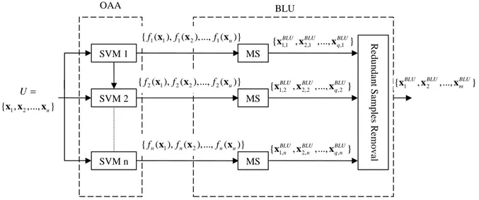
The binary-level uncertainty (BLU) technique separately selects a batch of the most uncertain unlabeled samples from each binary SVM on the basis of the MS query function. In the technique adopted in [12], only the unlabeled sample closest to the hyperplane of each binary SVM was added to the training set at each iteration (i.e., h=n). On the contrary, in the investigated BLU technique, at each iteration the most uncertain q (q>1) samples are selected from each binary SVM (instead of a single sample). In greater detail, n binary SVMs are initially trained with the current training set and the functional distance f x , i( ) i=1,...,n of each unlabeled sample x∈U to the hyperplane is obtained. Then, the set of q samples
{
x1,BLUi ,x2,BLUi ,...,xq iBLU,}
,1, 2,...,
i= n closest to margin of the corresponding hyperplane are selected for each binary SVM. Totally ρ=qn samples are taken. Note that xBLUj i, , j=1, 2,...,q, represents the selected j-th sample from the i-th SVM. Since some unlabeled samples can be selected by more than one binary SVM, the redundant samples are removed. Thus, the total number m of selected samples can actually be smaller than ρ (i.e., m≤ρ). The set of m most uncertain samples
1 2
{xBLU,xBLU,...,xBLUm } is forwarded to the diversity step. Fig. 1 shows the architecture of the investigated BLU technique.
Fig. 1. Multiclass architecture adopted for the BLU technique
Multiclass-Level Uncertainty (MCLU)
The adopted multiclass-level uncertainty (MCLU) technique selects the most uncertain samples according to a confidence value ( )c x , x∈U , which is defined on the basis of their functional distance f x , i( ) i=1,...,n to the n decision boundaries of the binary SVM classifiers
included in the OAA architecture [31], [33]. In this technique, the distance of each sample x∈U
to each hyperplane is calculated and a set of n distance values
{
f1( ),x f2( ),... ( )x fn x is obtained.}
Then, the confidence value ( )c x can be calculated using different strategies. Here, we consider
two strategies: 1) the minimum distance function cmin( )x strategy, which is obtained by taking the
smallest distance to the hyperplanes (as absolute value), i.e., [31]
{
}
min( ) imin1,2,...,n [ ( )] i c abs f = = x x (2)and 2) the difference cdiff( )x strategy, which considers the difference between the first largest and
the second largest distance values to the hyperplanes (note that, for the i-th binary SVM in the
OAA architecture, fi( )x ≥0 if x belongs to i-th class and fi( )x <0 if x belongs to the rest), i.e, [33]
{
}
{
}
1max 1max 2 max 1max 1,2,..., 2max 1,2,..., , arg max ( ) arg max ( ) ( ) ( ) ( ) i i n j j n j r diff r r r f r f c f f = = ≠ = = = − x x x x x (3) OAA BLU 1 1 1 2 1 { ( ),f x f(x ),...,f(xu)} 2 1 2 2 2 {f ( ),x f (x ),...,f (xu)} 1,1 2,1 ,1{ BLU, BLU,..., BLU}
q
x x x
1,2 2,2 ,2
{ BLU, BLU,..., BLU}
q
x x x
1, 2, ,
{ BLU, BLU,..., BLU}
n n q n x x x MS MS SVM 2 1 2 {fn( ),x fn(x ),...,fn(xu)} SVM n MS R ed u n d a n t S am p le s R em o v al 1 2 { , ,..., u} U= x x x SVM 1 1 2
{ BLU, BLU,..., BLU}
m
The cmin( )x function models a simple strategy that computes the confidence of a sample x taking
into account the minimum distance to the hyperplanes evaluated on the basis of the most uncertain binary SVM classifier. Differently, the cdiff( )x strategy assesses the uncertainty between the two
most likely classes. If this value is high, the sample x is assigned to r1max with high confidence. On the contrary, if cdiff( )x is small, the decision for r1max is not reliable and there is a possible conflict with the classr2max (i.e., the sample x is very close to the boundary between class r1max and r2max). Thus, this sample is considered uncertain and is selected by the query function for better modeling the decision function in the corresponding position of the feature space. After that the ( )c x value
of each x∈U is obtained based on one of the two above-mentioned strategies, the m samples
1 , 2 ,...,
MCLU MCLU MCLU m
x x x with lower ( )c x are selected to be forwarded to the diversity step. Note that
MCLU j
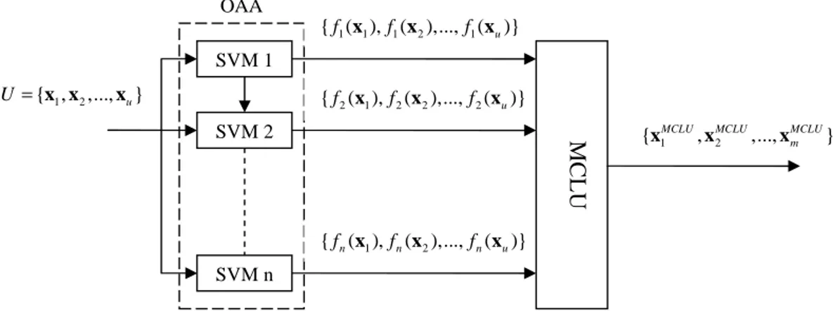
x denotes the selected j-th most uncertain sample based on the MCLU strategy. Fig. 2 shows the architecture of the investigated MCLU technique.
Fig. 2. Architecture adopted for the MCLU technique.
B. Techniques for Implementing the Diversity Criterion
The main idea of using diversity in AL is to select a batch of samples (h>1) which have low confidence values (i.e., the most uncertain ones), and at the same time are diverse from each other. In this paper, we consider two diversity methods: 1) the angle based diversity (ABD); and 2) the clustering based diversity (CBD). Before considering the multiclass formulation, in the following we recall their definitions for two-class problems.
Angle Based Diversity (ABD)
OAA M C L U 1 1 1 2 1 { ( ),f x f(x ),...,f(xu)} SVM 1 1 2
{xMCLU,xMCLU,...,xMCLUm }
2 1 2 2 2 {f ( ),x f (x ),...,f (xu)} 1 2 {fn( ),x fn(x ),...,fn(xu)} SVM 2 SVM n 1 2 { , ,..., u} U= x x x
A possible way for measuring the diversity of uncertain samples is to consider the cosine angle distance. It is a similarity measure between two samples defined in the kernel space by [13]
(
)
1 ( ) ( ) ( , ) cos ( , ) ( ) ( ) ( , ) ( , ) ( , ) ( , ) cos ( ) ( , ) ( , ) i j i j i j i j i i j j i j i j i i j j K K K K K K φ φ φ φ − ⋅ ∠ = = ∠ = x x x x x x x x x x x x x x x x x x x x (4)where ( )φ ⋅ is a nonlinear mapping function and K( , )⋅ ⋅ is the kernel function (see section II B). The cosine angle distance in the kernel space can be constructed using only the kernel function without considering the direct knowledge of the mapping function ( )φ ⋅ . The angle between two samples is small (cosine of angle is high) if these samples are close to each other and vice versa.
Clustering Based Diversity (CBD)
Clustering techniques evaluate the distribution of the samples in a feature space and group the similar samples into the same clusters. In [14], the standard k-means clustering [34] was used in the diversity step of binary SVM AL technique. The aim of using clustering in the diversity step is to consider the distribution of uncertain samples and select the cluster prototypes as they are more sparse in the feature space (i.e., distant one another). Since the samples within the same cluster are correlated and provide similar information, a representative sample is selected for each cluster. In [14], the sample that is closest to the corresponding cluster center (called medoid sample) is chosen as representative sample.
C. Proposed combination of Uncertainty and Diversity techniques generalized to Multiclass Problems
In this paper, each uncertainty technique is combined with one of the (binary) diversity techniques presented in the previous section. In the uncertainty step, the m most uncertain samples are selected using either MCLU or BLU. In the diversity step, the most diverse h<m samples are chosen based on either ABD or CBD generalized to the multiclass case. Here, four possible combinations are investigated: 1) MCLU with ABD (denoted by MCLU-ABD), 2) BLU with ABD (denoted by BLU-ABD), 3) MCLU with CBD (denoted by MCLU-CBD), and 4) BLU with CBD (denoted by BLU-CBD).
Combination of Uncertainty with ABD for Multiclass SVMs (MCLU-ABD and BLU-ABD)
In the binary AL algorithm presented in [13], the uncertainty and ABD criteria are combined based on a weighting parameterλ. On the basis of this combination, a new sample is included in the selected batch X according to the following optimization problem:
( , ) arg min ( ) (1 ) max
( , ) ( , ) i j i j X i I X i i j j K t f K K λ λ ∈ ∈ = + − x x x x x x x (5)
where
I
denotes the indices of unlabeled examples whose distance to the classification hyperplane is less than one, /I X represents the index of unlabeled samples of I that are not contained in X,λ provides the tradeoff between uncertainty and diversity, and t denotes the index of the unlabeled sample that will be included in the batch. The cosine angle distance between each sample of /I X
and the samples included in X is calculated and the maximum value is taken as the diversity value of the corresponding sample. Then, the sum of the uncertainty and diversity values weighted by λ is considered to define the combined value. The unlabeled samplex that minimizes such value is t
included in X. This process is repeated until the cardinality of X ( X ) is equal to h. This technique
guarantees that the selected unlabeled samples in X are diverse regarding to their angles to all the others in the kernel space. Since the initial size of X is zero, the first sample included in X is always the most uncertain sample of
I
(i.e., closest to the hyperplane). We generalize this technique to multiclass architectures presenting the MCLU-ABD and BLU-ABD algorithms.Algorithm 2: MCLU-ABD Inputs:
λ (weighting parameter that tune the tradeoff between uncertainty and diversity)
m (number of samples selected on the basis of their uncertainty) h (batch size)
Output:
X (set of unlabeled samples to be included in the training set)
1. Compute ( )c x for each sample x∈U .
2. Select the set of m unlabeled samples with lower c x value (most uncertain) ( )
1 2
{xMCLU,xMCLU,...,xMCLUm }.
3. Initialize X to the empty set.
4. Include in X the most uncertain sample (the one that has the lowest ( )c x value).
Repeat
5. Compute the combination of uncertainty and diversity with the following equation formulated for the multiclass architecture:
( , ) arg min ( ) (1 ) max
( , ) ( , ) i j i j X i I X i i j j K t c K K λ λ ∈ ∈ = + − x x x x x x x (6)
where
I
denotes the set of indices of m most uncertain samples and ( )c x is calculated asexplained in the MCLU subsection (with cmin( )x or cdiff( )x strategy).
6. Include the unlabeled samplex in X. t Until X =h
7. The supervisor S adds the label to the set of samples { 1MCLU ABD, 2MCLU ABD,..., MCLU ABD}
h X
− − − ∈
x x x
and these samples are added to the current training set T.
It is worth noting that the main difference between (5) and (6) is that the uncertainty in (6) is evaluated considering the confidence function ( )c x instead of the functional distance ( )i f x as in i
the binary case.
Algorithm 3: BLU-ABD Inputs:
λ(weighting parameter that tune the tradeoff between uncertainty and diversity)
m (number of samples selected on the basis of their uncertainty) h (batch size)
q (number of unlabeled samples selected for each binary SVM in the BLU technique) n (total class number)
Output:
X (set of unlabeled samples to be included in the training set)
1. Select the q most uncertain samples from each of the n binary SVM included in the multiclass OAA architecture (totally ρ=qnsamples are obtained).
2. Remove the redundant samples and consider the set of m≤ρ patterns { 1BLU, 2BLU,..., BLU}
m
x x x .
3. Compute ( )c x for the set of m samples as follows: if one sample is selected by more than one
binary SVM, ( )c x is calculated as explained in the MCLU subsection (with cmin( )x or cdiff( )x
strategy); otherwise ( )c x is assigned to the corresponding functional distance ( )f x .
4. Initialize X to the empty set.
5. Include in X the most uncertain sample (the one that has the lowest ( )c x value).
Repeat
6. Compute the combination of uncertainty and diversity with the equation (6). 7. Include the unlabeled samplex in X. t
Until X =h
8. The supervisor S adds the label to the set of patterns { 1BLU ABD, 2BLU ABD,..., BLU ABD}
h X
− − − ∈
x x x and
these samples are added to the current training set.
Combination of Uncertainty with CBD for Multiclass SVMs (MCLU-CBD and BLU-CBD)
Then, the standard k-means clustering is applied in the original feature space to the unlabeled samples whose distance to the hyperplane (computed in the kernel space) is less than one (i.e., those that lie in the margin) and the k=h clusters are obtained. The medoid sample of each cluster is added to X (i.e., X =h), labeled by the supervisor S and moved to the current training set. This algorithm evaluates the distribution of the uncertain samples within the margin and selects the representative of uncertain samples based on standard k-means clustering. We extend this technique to multiclass problems. Here we define the MCLU-CBD and BLU-CBD algorithms.
Algorithm 4: MCLU-CBD Inputs:
m (number of samples selected on the basis of their uncertainty) h (batch size)
Output:
X (set of unlabeled samples to be included in the training set)
1. Compute ( )c x for each sample x∈U .
2. Select the set of m unlabeled samples with lowest ( )c x (with cmin( )x or cdiff( )x strategy) value
(most uncertain) {x1MCLU,x2MCLU,...,xMCLUm }.
3. Apply the k-means clustering (diversity criterion) to the selected m most uncertain samples with
k=h.
4. Calculate the h cluster medoid samples { 1MCLU CBD, 2MCLU CBD,..., MCLU CBD}
h
− − −
x x x , one for each
cluster.
5. Initialize X to the empty set and include in X the set of h patterns
1 2
{ MCLU CBD, MCLU CBD,..., MCLU CBD}
h X
− − − ∈
x x x
6. The supervisor S adds the label to the set of h patterns {x1MCLU CBD− ,x2MCLU CBD− ,...,xhMCLU CBD− }∈X
Algorithm 5: BLU-CBD Inputs:
m (number of samples selected on the basis of their uncertainty) h (batch size)
q (number of unlabeled samples selected for each binary SVM in the BLU technique) n (total class number)
Output:
X (set of unlabeled samples to be included in the training set)
1. Select the q most uncertain samples from each of the n binary SVMs included in the multiclass OAA architecture (totally ρ=qnsamples are obtained).
2. Remove the redundant samples and consider the set of m≤ρ patterns {x1BLU,x2BLU,...,xmBLU}.
3. Compute ( )c x for the set of m samples as follows: if one sample is selected by more than one binary SVM, ( )c x is calculated as explained in the MCLU subsection (with cmin( )x or cdiff( )x
strategy); otherwise ( )c x is assigned to the corresponding functional distance ( )f x .
4. Apply the k-means clustering (diversity criterion) to the selected m most uncertain samples (k=h).
5. Calculate the h cluster medoid samples { 1BLU CBD, 2BLU CBD,..., BLU CBD}
h
− − −
x x x , one for each cluster. 6. Initialize X to the empty set and include in X the set of h patterns
1 2
{ BLU CBD, BLU CBD,..., BLU CBD}
h X
− − − ∈
x x x
7. The supervisor S adds the label to the set of h patterns { 1BLU CBD, 2BLU CBD,..., BLU CBD}
h X
− − − ∈
x x x and
these samples are added to the current training set.
IV. PROPOSED NOVEL QUERY FUNCTION
Clustering is an effective way to select the most diverse samples considering the distribution of uncertain samples in the diversity step of the query function. In the previous section we generalized the CBD technique presented in [14] to the multiclass case. However, some other limitations can compromise its application: 1) the standard k-means clustering is applied to the original feature space and not in the kernel space where the SVM separating hyperplane operates, and 2) the medoid sample of each cluster is selected in the diversity step as the corresponding cluster representative sample (even if “more informative” samples in that cluster could be selected).
To overcome these problems, we propose a novel query function that is based on the combination of a standard uncertainty criterion for multiclass problems and a novel Enhanced CBD (ECBD) technique. In the proposed query function, MCLU is used with the difference
( )
diff
c x strategy in the uncertainty step to select the m most uncertain samples. The proposed ECBD technique, unlike the standard CBD, works in the kernel space by applying the kernel k-means clustering [35], [36] to the m samples obtained in the uncertainty step to select the h<m
clusters (C C1, 2,...C ) in the kernel space. At the first iteration, initial clusters h C C1, 2,...C are h
constructed assigning initial cluster labels to each sample [35]. In next iterations, a pseudo centre is chosen as the cluster center (the cluster centers in the kernel space
φ µ φ µ
( ) ( )
1 , 2 ,...φ µ
( )
h can not be expressed explicitly). Then the distance of each sample from all cluster centers in the kernel space is computed and each sample is assigned to the nearest cluster. The Euclidean distance betweenφ
( )
xi andφ µ
( )
v , v=1, 2,...,h, is calculated as [35], [36]:2 2 2 1 1 2 1 1 ( ( ), ( )) ( ) ( ) 1 ( ) ( ( ), ) ( ) 2 ( , ) ( ( ), ) ( , ) 1 ( ( ), ) ( ( ), ) ( ) i v i v m i j v j j v m i i j v i j j v m m j v l v j l j l v D C C K C K C C C K , C φ φ µ φ φ µ φ δ φ φ δ φ δ φ δ φ = = = = = − = − = − +
∑
∑
∑∑
x x x x x x x x x x x x x x (7)where
δ φ
(
(xj),Cv)
shows the indicator function. Theδ φ
(
(xj),Cv)
=1 only if x is assigned to j vC , otherwise
δ φ
(
(xj),Cv)
=0. The Cv denotes the total number of samples in C and is vcalculated as
(
)
1 ( ), m v j v j C δ φ C ==
∑
x . As mentioned before, ( )φ ⋅ is a nonlinear mapping function from the original feature space to a higher dimensional space and K( , )⋅ ⋅ is the kernel function. The kernel k-means algorithm can be summarized as follows [35]:1. The initial value of
δ φ
(( )
xi ,Cv), i=1, 2,...,m, v=1, 2,...,h, is assigned and h initial clusters{
C C1, 2,...Ch}
are obtained.2. Then xi is assigned to the closest cluster.
( )
1 if 2( ( ), ( )) 2( ( ), ( )) j ( , ) 0 otherwise i v i j i v D D v C φ φ µ φ φ µ δ φ = < ∀ ≠ x x x (8)3. The sample that is closest toµv is selected as the pseudo centre ηv of C . v
( )
arg min ( , ( )) i v v i v C D η φ φ µ ∈ = x x (9)4. The algorithm is iterated until converge, which is achieved when samples do not change clusters anymore.
After C C1, 2,...C are obtained, unlike in the standard CBD technique, the most informative h
(i.e., uncertain) sample is selected as the representative sample of each cluster. This sample is defined as
( )
{
}
arg min ( ) 1, 2,...,
i v
MCLU ECBD MCLU
v diff i C c v h φ − ∈ = = x x x (10)
where MCLU ECBD v
−
x represents the v-th sample selected using the proposed query function MCLU-ECBD and is the most uncertain sample of the v-th cluster (i.e., the sample that has minimum
( )
diff
c x in the v-th cluster). Totally h samples are selected, one for each cluster, using (10).
In order to better understand the difference in the selection of the representative sample of each cluster between the query function presented in [14] (which selects the medoid sample as cluster representative) and the proposed query function (which selects the most uncertain sample of each cluster), Fig. 3 presents a qualitative example. Note that, for simplicity, the example is presented for binary SVM in order to visualize the confidence value cdiff( )x as the functional
distance (MS is used instead of MCLU). The uncertain samples are firstly selected based on MS for both techniques, and then the diversity step is applied. The query function presented in [14] selects medoid sample of each cluster (reported in blue in the figure), which however is not in agreement with the idea to select the most uncertain sample in the cluster. On the contrary, the proposed query function considers the most uncertain sample of each cluster (reported in red in the figure). This is a small difference with respect to the algorithmic implementation but a relevant difference from a theoretical viewpoint and for possible implications on results.
(a) (b)
The proposed MCLU-ECBD algorithm can be summarized as follows:
Algorithm 6: Proposed MCLU-ECBD Inputs:
m (the number of samples selected on the basis of their uncertainty) h (batch size)
Output:
X (set of unlabeled samples to be included in the training set)
1. Compute ( )c x for each sample x∈U .
2. Select the set of m unlabeled samples with lower c x value (most uncertain) ( )
1 2
{ MCLU, MCLU,..., MCLU}
m
x x x .
3. Apply the kernel k-means clustering (diversity criterion) to the selected m most uncertain samples with k=h.
4. Select the representative sample MCLU ECBD v
−
x ,v=1, 2,…,h (i.e., the most uncertain sample) of each cluster according to (10).
5. Initialize X to the empty set and include in X the set of samples MCLU ECBD
v X
− ∈
x , v=1, 2,…,h. 6. The supervisor S adds the label to the set of samples xvMCLU ECBD− ∈X , v=1, 2,…,h, and these samples are added to the current training set.
V. DATA SET DESCRIPTION AND DESIGN OF EXPERIMENTS
A. Data set description
Two data sets were used in the experiments. The first data set is a hyperspectral image acquired on a forest area on the Mount Bondone in the Italian Alps (near the city of Trento) on September 2007. This image consists of 1613 1048× pixels and 63 bands with a spatial resolution of 1 m. The available labeled data (4545 samples) were collected during a ground survey in summer 2007. The reader is referred to [37] for greater details on this dataset. The samples were randomly divided to derive a validation set V of 455 samples (which is used for model selection), a test set TS of 2272 samples (which is used for accuracy assessment), and a pool P of 1818 samples. The 4 % of the samples of each class are randomly chosen from P as initial training samples and the rest are considered as unlabeled samples. The land cover classes and the related number of samples used in the experiments are shown in Table 1.
The second data set is a Quickbird multispectral image acquired on the city of Pavia (northern Italy) on June 23, 2002. This image includes the four pan-sharpened multispectral bands and the panchromatic channel with a spatial resolution of 0.7 m. The image size is 1024 1024× pixels. The reader is referred to [38] for greater details on this dataset. The available labeled data (6784 samples) were collected by photointerpretation. These samples were randomly divided to
derive a validation set V of 457 samples, a test set TS of 4502 samples and a pool P of 1825 samples. According to [38], Test pixels were collected on both homogeneous areas TS1 and edge
areas TS2 of each class. The 4 % of the samples of each class in P are randomly selected as initial
training samples, and the rest are considered as unlabeled samples. Table 2 shows the land cover classes and the related number of samples used in the experiments.
TABLE 1.NUMBER OF SAMPLES OF EACH CLASS IN P,V AND TS FOR THE TRENTO DATA SET.
Class P V TS Fagus Sylvatica 720 180 900 Larix Decidua 172 43 215 Ostrya Carpinifolia 160 40 200 Pinus Nigra 186 47 232 Pinus Sylvestris 340 85 425 Quercus Pubescens 240 60 300 Total 1818 455 2272
TABLE 2.NUMBER OF SAMPLES OF EACH CLASS IN P,V,TS1 AND TS2 FOR THE PAVIA DATA SET.
Class P V TS1 TS2 Water 58 14 154 61 Tree areas 111 28 273 118 Grass areas 103 26 206 115 Roads 316 79 402 211 Shadow 230 57 355 311 Red buildings 734 184 1040 580 Gray buildings 191 48 250 177 White building 82 21 144 105 Total 1825 457 2824 1678 B. Design of Experiments
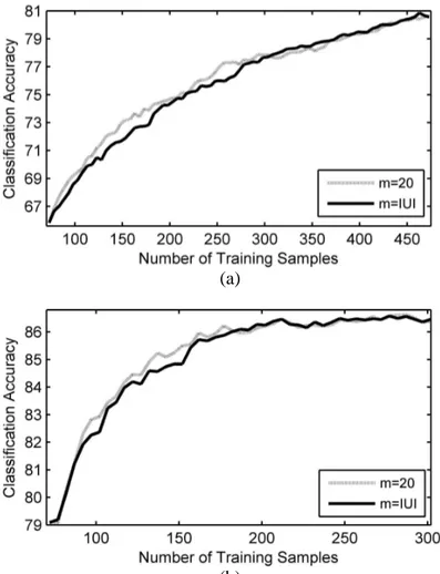
In our experiments, without loosing in generality, we adopt an SVM classifier with RBF kernel. The values for C and γ parameters are selected performing a grid-search model selection only at the first iteration of the AL process. Indeed, initial experiments revealed that, if a reasonable number of initial training samples is considered, performing the model selection at each iteration does not increase significantly the classification accuracies at the cost of a much higher computational burden. The MCLU step is implemented with different m values, defined on the basis of the value of h (i.e., m=4 , 6 , 10h h h), with h=5,10,40,100. In the BLU technique, the q=h most uncertain samples are selected for each binary SVM. Thus the total number of selected samples for all SVMs isρ=qn. After removing repetitive patterns, m≤ρ samples are obtained. The value of λ used in the MCLU-ABD and the BLU-ABD [for computing (6)] is varied as
means clustering is fixed to h. All the investigated techniques and the proposed MCLU-ECBD technique are compared with the EQB and the MS-cSV techniques presented in [12]. The results of EQB are obtained fixing the number of EQB predictors to eight and selecting bootstrap samples containing 75 % of initial training patterns. These values have been suggested in [12]. Since the MS-cSV technique selects diverse uncertain samples according to their distance to the SVs, and can consider at most one sample related to each SV, it is not possible to define h greater than the total number of SVs. For this reason we can provide MS-cSV results for only h=5,10. Also the results obtained by the KL-Max technique proposed in [32] are provided for comparison purposes. Since the computational complexity of KL-Max implemented with SVM is very high, in our experiments at each iteration an unlabeled sample is chosen from a randomly selected subset (made up of 100 samples) of the unlabeled data. Note that the KL-Max technique can be implemented with any classifier that exploits posterior class probabilities for determining the decision boundaries [32]. In order to implement KL-Max technique with SVM, we converted the outputs of each binary SVM to posterior probabilities exploiting the Platt’s method [39].
All experimental results are referred to the average accuracies obtained in ten trials according to ten initial randomly selected training sets. Results are provided as learning rate curves, which show the average classification accuracy versus the number of training samples used to train the SVM classifier. In all the experiments, the size of final training set T is fixed to 473 for the Trento data set, and to 472 for the Pavia data set. The total number of iterations is given by the ratio between the number of samples to be added to the initial training set and the pre-defined value of h.
VI. EXPERIMENTAL RESULTS
We carried out different kinds of experiments in order to: 1) compare the effectiveness of the different investigated techniques that we generalized to the multiclass case in different conditions; 2) assess the effectiveness of the novel ECBD technique; 3) compare the investigated methods and the proposed MCLU-ECBD technique with the techniques used in the RS literature; and 4) perform a sensitivity analysis with respect to different parameter settings and strategies.
A. Results: Comparison among Investigated Techniques Generalized to the Multiclass Case
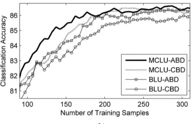
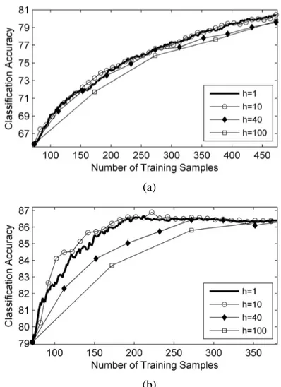
In the first set of trials, we analyze the effectiveness of the investigated techniques generalized to multiclass problems. As an example, Fig. 4 compares the overall accuracies versus the number of initial training samples obtained by the MCLU-ABD, the MCLU-CBD, the
BLU-ABD and the BLU-CBD techniques with h=5, k=5 andλ=0.6. In the MCLU, m=20 samples are selected for both data sets. In the BLU, m≤30and m≤40 samples are chosen for the Trento and Pavia data sets, respectively. The confidence value is calculated with the cdiff( )x strategy for both
MCLU and BLU, as preliminary tests pointed out that by fixing the query function, the cdiff( )x
strategy is more effective than the cmin( )x strategy in case of using MCLU, whether it provides
similar classification performance to the cmin( )x strategy when using BLU. Fig. 4 shows that the
MCLU-ABD technique is the most effective on both the considered data sets. Note that similar behaviors are obtained by using different values of parameters (i.e., m, h,λand k). The effectiveness of the MCLU and BLU techniques for uncertainty assessment can be analyzed by comparing the results obtained by combining them with the same diversity techniques under the same conditions (i.e., same values for parameters). From Fig. 4, one can observe that the MCLU technique is more effective than the BLU in the selection of the most uncertain samples on both data sets (i.e., the average accuracies provided by the MCLU-ABD are higher than those obtained by the BLU-ABD and a similar behavior is obtained with the CBD). This trend is confirmed by using different values of parameters (i.e., m, h,λand k ). The ABD and CBD techniques can be compared by combining them with the same uncertainty technique under the same conditions (i.e., same values for parameters). From Fig. 4, one can see that the ABD technique is more effective than the CBD technique. The same behavior can also be observed by varying the values of parameters (i.e., m, h,λand k ).
(b)
Fig. 4. Overall classification accuracy obtained by the MCLU and BLU uncertainty criteria when combined with the ABD and CBD diversity techniques in the same conditions for (a) Trento, and b) Pavia data sets. The learning curves are reported starting from 183 samples and 87 samples for Trento and Pavia data sets,
respectively, in order to better highlight the small differences.
B. Results: Proposed MCLU-ECBD Technique
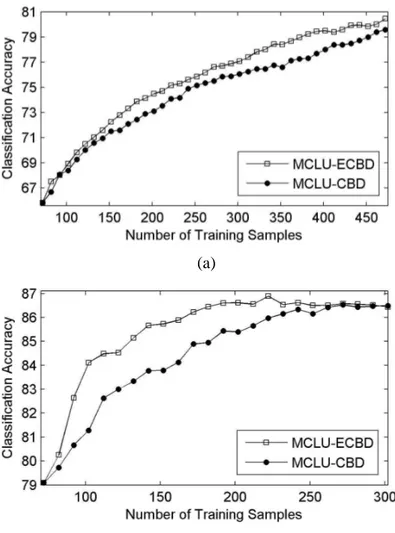
In the second set of trials, we compare the standard CBD with the proposed ECBD using the MCLU uncertainty technique with the cdiff( )x strategy and fixing the same parameter values. As
an example, Fig. 5 shows the results obtained with m=40,h=10,k =10 for both data sets. Table 3 (Trento data set) and Table 4 (Pavia data set) report the mean and standard deviation of classification accuracies obtained on ten trials versus different iteration numbers and different training data sizeT . From the reported results, one can see that ECBD technique provides the selection of more informative samples compared to CBD technique achieving higher accuracies than the standard CBD algorithm for the same number of samples. In addition, it can reach the convergence in less iterations. These results are also confirmed in other experiments with different values of parameters (not reported for space constraints).
(a)
(b)
Fig. 5. Overall classification accuracy obtained by the MCLU uncertainty criterion when combined with the standard CBD and the proposed ECBD diversity techniques for (a) Trento, and (b) Pavia data sets.
TABLE 3.AVERAGE CLASSIFICATION ACCURACY (CA) AND STANDARD DEVIATION (STD) OBTAINED ON TEN TRIALS FOR DIFFERENT TRAINING DATA SIZE T AND ITERATION NUMBERS (ITER.NUM)(TRENTO DATA SET) T = 163 (Iter.Num. 9) T = 193 (Iter. Num. 12) T = 333 (Iter. Num. 26) Technique CA std CA std CA std Proposed MCLU-ECBD 72.78 1.20 74.13 1.42 78.00 1.00 MCLU-CBD 71.55 1.57 72.88 1.62 76.47 1.10
TABLE 4.AVERAGE CLASSIFICATION ACCURACY (CA) AND STANDARD DEVIATION (STD) OBTAINED ON TEN TRIALS FOR DIFFERENT ITERATION NUMBERS (ITER.NUM) AND TRAINING DATA SIZE T (PAVIA DATA SET)
T = 102 (Iter.Num. 3) T = 142 (Iter. Num. 7) T = 172 (Iter. Num. 10) Technique CA std CA std CA std Proposed MCLU-ECBD 84.10 1.66 85.66 1.29 86.23 1.09
C) Results: Comparison among the Proposed AL Techniques and Literature Methods
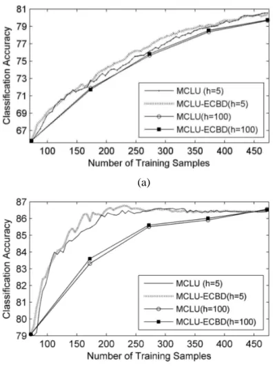
In the third set of trials, we compare the investigated and proposed techniques with AL techniques proposed in the RS literature. We compare the MCLU-ECBD and the MCLU-ABD techniques with the MS-cSV [31], the EQB [31] and the KL-Max [32] methods. According to the accuracies presented in section VA, we present the results obtained with the MCLU, which is more effective than the BLU. Fig. 6 shows the average accuracies versus the number of training samples obtained in the case of h=5 (h=1 only for KL-Max) for both data sets. For a fair comparison, the highest average accuracy result of each technique is given in the figure. Note that, since the MCLU-CBD proved less accurate than the MCLU-ECBD (see section V B), its results are no more reported here. For the Trento data set, the highest accuracies for MCLU-ECBD are obtained with m=30 (while k=5), whereas the best results for MCLU-ABD are obtained with λ=0.6 and
20
m= . For the Pavia data set, the highest accuracies for MCLU-ECBD are obtained with 20
m= (while k=5), whereas the best results for MCLU-ABD are obtained with λ=0.6 and 20
m= .
By analyzing Fig. 6a (Trento data set) one can observe that MCLU-ECBD and MCLU-ABD results are much better than MS-cSV, EQB, KL-Max results. The accuracy value at convergence of the EQB is significantly smaller than those of other techniques. The KL-Max accuracies are similar to the MS-cSV accuracies at early iterations. However, the accuracy of the KL-Max at convergence is smaller than those of the MCLU-ECBD and MCLU-ABD, as well as those of other methods. The results obtained on the Pavia data set (see Fig. 6b) show that the proposed MCLU-ECBD technique leads to the highest accuracies in most iteration; furthermore, it achieves convergence in less iterations than the other techniques. The MCLU-ABD method provides slightly lower accuracy than MCLU-ECBD; however, it results in significantly higher accuracies than MS-cSV, EQB as well as KL-Max techniques. KL-Max accuracy at convergence is significantly smaller than those achieved with other techniques.
For a better comparison, additional experiments were carried out on both data sets varying the values of the parameters. In all cases, we observed that MCLU-ECBD and MCLU-ABD yield higher classification accuracies than the other AL techniques when small h values are considered, and that the EQB technique is not effective when selecting a small number h of samples. On the contrary, the accuracies of EQB are close to those of MCLU-ECBD and MCLU-ABD when relatively high h values are considered. MS-cSV can not be used for high h values when small initial training set are available since the maximum number of h is equal to the total number of
SVs. KL-Max results can only be provided for h=1 and the related accuracies are smaller than those of both MCLU-ECBD and MCLU-ABD methods.
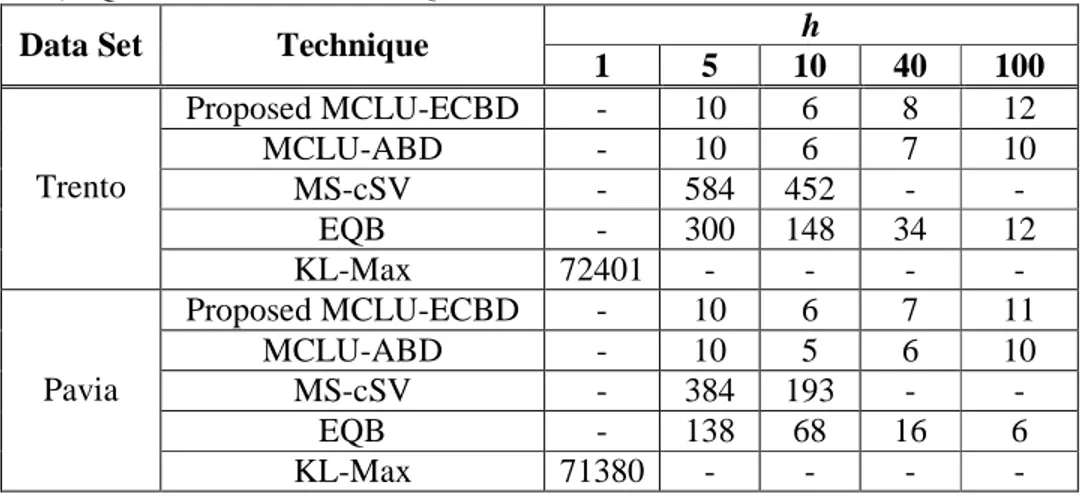
Table 5 reports the computational time (in seconds) required by ECBD, MCLU-ABD, MS-cSV, and EQB (for one trial) for different h values, and the computational time taken from KL-Max (related to h=1) for both data sets. In this case, the value of m for MCLU-ECBD and ABD is fixed to 4h for both data sets. It can be noted that ECBD and MCLU-ABD are fast both for small and high values of h. The computational time of MS-cSV and EQB is very high in the case of small h values, whereas it decreases by increasing the h value. The largest computational time is obtained with KL-Max that with an SVM classifier requires the use of the Platt algorithm for computing the class posterior probabilities. All the results clearly confirm that on the two considered data sets the proposed MCLU-ECBD is the most effective technique in terms of both computational complexity and classification accuracy.
(a)
(b)
![Fig. 3. Comparison between the samples selected by (a) the CBD technique presented in [14],](https://thumb-eu.123doks.com/thumbv2/123dokorg/2946532.22920/21.918.123.746.709.1026/fig-comparison-samples-selected-cbd-technique-presented.webp)