ALEA
Tech Reports
Determinants of the implied volatility
function on the Italian Stock Market
Alessandro Beber
Tech Report Nr. 10
Marzo 2001
Alea - Centro di ricerca sui rischi finanziari
Dipartimento di informatica e studi aziendali
Università di Trento - Via Inama 5 - 38100 - Trento
http://www.aleaweb.org/
nicola
ALEA, Centro di ricerca sui rischi finanziari è un centro di ricerca indipendente costituito presso il Dipartimento di informatica e studi aziendali dell'Università di Trento. Il centro si propone di elaborare conoscenze innovative in materia di risk management, e di favorirne la diffusione mediante pubblicazioni e programmi di formazione. Il centro è diretto dal prof. Luca Erzegovesi. Nella collana ALEA Tech Reports sono raccolti lavori di compendio e rassegna della letteratura e della prassi operativa su tematiche fondamentali di risk management.
Alessandro Beber(*)
Determinants of the implied volatility
function on the Italian Stock Market
Abstract
This paper describes the implied volatility function computed from options on the Italian stock market index between 1995 and 1998 and tries to find out potential explanatory variables. We find that the typical smirk observed for S&P500 stock index characterizes also Mib30 stock index. When potential determinants are investigated by a linear Granger Causality test, the important role played by option’s time to expiration, transacted volumes and historical volatility is detected. A possible proxy of portfolio insurance activity does poorly in explaining the observed pattern. Further analysis shows that the dynamic interrelation between the implied volatility function and some determinants could be, to a certain extent, non-linear.
JEL classification: G10; G12 ; G13.
First draft: July 2000
This revision: February 2001
(*) LEM – Laboratory of Economics and Management, St. Anna School of Advanced Studies, Pisa – Italy. Visiting scholar – Department of Finance, The Wharton School – University of Pennsylvania, Philadelphia – USA
The author acknowledges the helpful comments and suggestions of Carlo Bianchi, Luca Erzegovesi, Kenneth Kavajecz. Any remaining errors are the author’s responsibility. Please e.mail comments and suggestions to: [email protected].
Summary
1. Introduction ... 5
2. Data and sampling procedure ... 7
3. The implied volatility function... 14
4. Identifying the potential determinants... 17
5. Conclusions ... 23
References ... 25
Figures ... 28
1.
Introduction
Since October 1987 stock market crash, it is well known that implied volatilities computed from options on stock market indices using Black and Scholes (1973) formula vary across strike prices and maturities. In particular, on the US stock market, a decreasing profile of implied volatility with respect to moneyness has been invariably observed1; this is the so-called “volatility smile” or “smirk”, owing to asymmetric shape. As regards European stock markets, there is evidence of similar patterns, e.g. for the German equity market as illustrated by Tompkins (1999), but also of fairly symmetric “volatility smiles”, as pointed out by Pena et al. (1999) for the Spanish index.
Given the assumptions of Black and Scholes model, all the options with the same maturity and on the same underlying asset should have the same implied volatility, notwithstanding different strike prices; the presence of a volatility smile determines the roughness of Black and Scholes formula in the valuation of options with different moneyness.
Financial literature handled this empirical evidence of not constant implied volatility with two broad classes of methods. The first could be labelled “deterministic volatility methods”; in general it refers to the use of a pricing model in which the parameter of constant volatility is replaced by a deterministic volatility function: different examples of this type of models are the approach of Shimko (1993), the implied binomial tree or lattice approach developed by Derman and Kani (1994) and Rubinstein (1994), the non-parametric kernel regression approach of Ait-Sahalia and Lo (1998). The second class of methods could be labelled “two factors models”; besides the risk of the market price of underlying asset, the valuation models price additional non-traded sources of risk, such as the volatility of volatility or market price jumps or even both. One of the first examples belonging to this general class was the stochastic volatility model of Hull and White (1987); more recent advances are, among others, the stochastic volatility model of Heston (1993), the random jump model of Bates (1996) and the multifactor model of Bates (2000).
The relation between the implied volatility smile and some potential explanatory variables is examined for the Italian options market. This study differs from previous research along two primary dimensions. First, in order to get a reliable evidence of the smile shape during the examined period, I perform an extensive analysis considering different subperiods, different sets
1 See among the others Rubinstein (1994), Jackwerth and Rubinstein (1996), Dumas et al. (1998) who
illustrated that the implied volatility of the S&P500 index options decreases monotonically as the strike price increases with respect to the current level of the underlying asset.
of options and different measures of moneyness. The aim is to establish whether the smile’s profile is characterized by a negative slope, as in the US market, or whether it is symmetric, like the smile observed on the Spanish options market.
A second difference relative to previous work is that I try to find out potential determinants of the shape of the volatility smile; the direct explanation of these determinants has been an omitted topic in the extant literature. A formal categorization of explanatory variables can help not only to improve options’ pricing models, but also to enhance the methodologies extracting probability density function of the underlying from option prices2. I follow the methodological approach of Pena et al. (1999), who employed a linear Granger causality test to characterize the relation between the parameters of the interpolated volatility function and some explanatory variables; however this study differs substantially in the specific choice of the potential determinants and in the inference drawn from the findings. Moreover the analysis is extended through a non-linear Granger causality test.
The empirical results show that on the Italian options market a persistent asymmetric implied volatility function is observed, similar to the US evidence. This phenomena is well approximated by a simple quadratic function of moneyness, with a negative linear term and a small degree of convexity. When I try to relate the smile shape to potential determinants, I find that a prominent role is played by time to expiration, liquidity of the option market and historical volatility. A non-linear effect on the implied volatility function is present for all the explanatory variables employed in this analysis.
The paper is organized as follows. Section 2 discusses briefly the features of the Italian options market, describes data and explanatory variables employed in the analysis and provide descriptive statistics for these series. The revealed volatility smile is illustrated in Section 3 and an interpreting model is derived. Section 4 explains the theoretical framework of the linear and non-linear Granger causality tests and presents the empirical results for potential determinants. Finally Section 5 offers a brief summary and provides conclusions and suggested areas for further research.
2
For a comprehensive survey of the literature about probability density function implied by option prices, see Jackwerth (1999).
2.
Data and sampling procedure
This empirical analysis focuses on Mibo30 stock index options and on some potential explanatory variables extrapolated either from the same market or from the market for the underlying asset.
2.1
Italian Mibo30 Index options
Mibo30 are options written on the Italian stock market index Mib30, which comprises the 30 most liquid and capitalized stocks; they were introduced on the Italian Derivatives Market (IDEM) on the 15th of November 1995. The volume traded on Mibo30 options represented 46% of the volume traded on all Italian equities in 1996, 72% in 1997 and 63% in 1998; the Mibo30 number of contracts relative to the French and Spanish stock index options was respectively 24% and 136% in 1997.
Mibo30 options are european style options, which means that exercise is possible only at maturity. The market price is stated in index points, each one worth 2.5 euro (called contract
multiplier). The contract dimension (notional value) is determined by the product between the multiplier and the strike price (expressed in index points).
Mibo30 options contracts have supplementary expiration dates with respect to the correspondent Fib30 future contract: besides quarterly maturities, there are also monthly maturities. The option contract expires the third Friday of the expiration month at 9.30 a.m. For each maturity, nine different strike prices are quoted: four out of the money, four in the money and one at the money. The lowest price interval between strike prices is fixed at 500 index-points.
The closing prices are determined daily by the Clearing House (Cassa di Compensazione e Garanzia). The settlement price corresponds to the value of Mib30 index calculated on expiration date’s opening prices of the 30 stocks composing the index. The contract settlement is carried out by cash as the difference between option’s strike price and Mib30 settlement price, taking into account the number of contracts, the multiplier value and by means of the Clearing
House.
2.2
Sampling procedure
The dataset is composed by the closing prices of call and put options on the Mib30 Index traded daily on IDEM during the period November 1995-March 19983.
3 I gratefully acknowledge the Italian Stock Market “Borsa Italiana SpA” for making available the
In order to consider only liquid prices, which is an extremely important issue when high frequency data are not available, the daily set of observations is filtered according to four criteria.
First, the closing prices of options with no transactions during the trading day are taken out of sample. Second, the dataset is filtered to include only calls and puts with the same expiration date of the corresponding stock index future. Hence I consider only the March, June, September and December maturity; in the dataset the average monthly transaction volume for options with quarterly expiration dates turns out to be about 12% higher than the average transaction volume on options with monthly maturities.
The third criteria is to exclude options with less than 5 and more than 90 trading days to expiration, which may induce liquidity-related biases. The shorter term options have relatively small time premiums, hence the estimation of volatility is extremely sensitive to any possible measurement error, particularly if options are not at the money, as Hentschel (2000) shows; other liquidity biases can arise for example because of fund manager’s positions rolling over. The longer term options, on the other hand, are simply less traded4.
Finally, arbitrage exclusion criteria are employed in order to avoid errors or microstructure effects such as non synchronous prices between options and the underlying5.
This filtering procedure reduces the data from 20146, corresponding to 600 trading sessions, to 7963 observations (3600 for call and 4363 for put options), with an average of 13 liquid prices per day. Moreover in the most relevant part of this study only out of the money put and call options are going to be employed: thus the more involved and active part of the market is considered (e.g. the portfolio insurance activity or the sale of covered call by fund managers). For instance in this dataset the average daily number of contracts on the out of the money options is nearly twice the volume on the in the money options. In this way the dataset is reduced to 4818 observations, with an average of 8 liquid prices per day.
Even if the underlying of the Mibo30 options is the Mib30 stock cash index, in this analysis I consider the prices of the corresponding future Fib30 and the Black (1976) version of the option
4 Similar exclusionary criteria are applied among others by Bakshi et. al (1997) or by Dumas et al. (1998). 5 The value of a European call option like the Mibo30 considered in this analysis should respect the
following applied boundary and strike price conditions:
C ≥ max (0, (F - K)R-t ); C(K
1)>C(K2) where K1<K2 ; (K2-K1)R-t≥ C(K1)-C(K2)>0 .
where C is the call price, K is the strike price, F is the forward price and R is a capitalization factor. I apply the same arbitrage exclusionary criteria to put options.
pricing formula6. This approach is far more simple, because the estimation of the dividend yield which is compounded in the price of the future contract can be avoided. Moreover during the period under analysis (Nov. 1995 – Mar. 1998) the settlement price of Mib30 stock index was non synchronous with respect to the derivatives market: in fact the closing price of Mib30 index was fixed at 5.00 p.m. while IDEM closed at 5.30 p.m.. For this reason considering a future price instead of an index price as underlying eliminates a large measurement error typically coming from using closing prices for the options and index that are measured half an hour apart (Hentschel, 2000).
From each observed option closing price Cit I compute implied volatility σit by numerically
solving the Black (1976) formula:
( )
[
( )
( )
]
(
)
(
)
t
T
d
d
t
T
t
T
K
F
d
d
K
d
F
e
C
it it it t t t T r it−
−
=
−
−
+
=
−
=
− −σ
σ
σ
1 2 2 1 2 12
ln
N
N
where, as usual, K is the strike price, Ft is the future price at time t, T is option’s expiration date,
r is the risk free interest rate and N represents the normal cumulative density function.
To proxy the risk free interest rate I use the one-month interbank interest rate for options with residual time to maturity between 5 and 45 trading days and the two month interbank interest rate for options with residual time to maturity between 45 and 90 trading days.
Options’ moneyness is computed with three alternative methodologies. First, I take the ratio of the strike price to the underlying future price7, following the frequent market convention of quoting (and hedging) the options in term of the future rather than the cash index. This method is straightforward, but it doesn’t consider that moneyness should be evaluated considering also the volatility of underlying asset and the option’s time to maturity. For this reason the second approach to moneyness takes into account explicitly these variables: the natural logarithm of the
6 At the maturity of the future, the future price equals the asset’s spot price. Thus a European option on
the asset has the same value as a European option on the future contract with the same maturity. As a result the Black and Scholes formula can be rewritten as shown by Black (1976) and afterwards in this section.
ratio of the strike price on the underlying future price is divided by the product of at the money implied volatility and the square root of the time to maturity8:
t
T
F
K
t atm t it−
,ln
σ
To compute at the money implied volatility I use the average of implied volatility of a call and a put option with a strike price K* as close as possible to index level, such that:
1
min
arg
*
=
S
K
−
K
t KThe third approach to compute moneyness is to use directly the options’ Delta. This measure considers in fact both time to maturity and volatility and at the same time is coherent with the Black and Scholes model. To avoid dependencies between the measure of moneyness and the implied volatility of options with different strike prices, at the money implied volatility is inserted in the Delta’s formula for each option as the volatility input.
It is convenient to normalize option’s Delta between zero and one in order to represent in the same way either call and put options; this can be achieved taking the absolute value of put option’s Delta and the complement to one of call option’s Delta, so as to obtain normalized values that increase with the strike.
In the reminder of this study I employ mainly this normalized Delta as the measure of moneyness, even if the robustness of the results is always checked also with the other two measures of moneyness.
2.3
Potential determinants definition
I look for the potential determinants of the volatility smile’ profile among three categories of variables. First, the specific features of the options market is illustrated, in order to obtain a reasonable estimate of general liquidity and potential links between smile effect and implied volatility term structure; hence I aim to explain options’ mispricings with the existence of market frictions. Second, the underlying asset dynamic is represented, in order to detect likely dependencies between the implied volatility function and relevant characteristics of the
8
Similar methodologies to compute moneyness are used in Natenberg (1994), Dumas et. al (1998), Tompkins (1999).
underlying asset9; options’ mispricings are explained by an investor assessments of the underlying stochastic process which is different from Black and Scholes hypothesis. Finally, I try to describe investors behavior, in order to reflect market practises which could have an impact on the implied volatility function as a consequence of relative trading activity in calls
versus puts of all strike prices; thus, as argued by option market practitioners, heavy demand for
out of the money put options drives up prices.
In the first category of options’ market specific variables the option’s residual time to expiration is employed, calculated as the ratio between the number of working days to the expiration date and the conventional working days in one year (252):
252
date
trading
date
expiration
−
=
tTEXP
Clearly I am trying to take into account the potential effect of the time horizon on the implied risk neutral density function.
The volume of transactions on options is also used, expressed as the simple number of traded contracts and either as number of traded options weighted by the value of the specific option’s contract10:
∑
==
m i i tn
NOPT
1∑
==
m i i i tc
n
K
VOPT
1where ni is the number of contracts traded on i-option, Ki is the i-option strike price, c is a
constant scaling factor and m is the number of different options traded each day of the sample. I want to proxy the liquidity in the market in the most general way.
The explanatory variables of the second category representing underlying asset’s dynamic are the market momentum, calculated as the natural logarithm of the ratio between the future price (Fib30) and a 50-day simple moving average:
∑
− ==
t t i i t tF
F
MOM
4950
1
ln
9 I don’t employ any variable related to interest rates owing to the small pricing improvement which is
usually obtained for stock index options when a time varying interest rates is considered. See among others Bakshi et al. (1997).
where Ft is the future price at time t. This ratio is positive (negative) in a bullish (bearish)
market11. Even if this measure is something like arbitrary, the aim is to gauge if the trend of the underlying has any effects on the steepness of the smile profile, given that it is well known that a leverage effect is present for the general level of volatility (e.g. Schwert (1989)).
A second potential explanatory variable is the volume of market transactions, expressed as the number of contracts traded each day on the stock index future contract (NFUTt); this is taken as
a measure of the general market activity in the underlying. This variable is correlated with conditional volatility and can influence the leverage effect (Gallant et. al. (1992)).
The level of historical volatility is also considered, calculated during the previous 20 trading days as the annualised standard deviation of logarithmic returns on Fib30 settlement prices:
(
)
[
,...,
−19]
252
=
t tt
r
r
HVOL
σ
where σ(x,…,y) is the standard deviation of values between x and y and rt is the daily
logarithmic return on Fib30 settlement prices. The potential effect of different levels of volatility on the smile profile would suggest that an obvious pricing improvement is to relax the assumption of constant volatility.
As a last variable of the second category the volatility of volatility is employed, computed during the previous 20 trading days like the standard deviation of the historical volatility shown before:
(
)
[
,...,
−19]
=
t t tHVOL
HVOL
VVOL
σ
where σ(x,…,y) is the standard deviation of values between x and y. This variable could be a
good proxy for the vega risk in hedging activity, that may affect the pricing of certain type of options.
The third category of potential determinants related to investor behaviour comprises one variable: the number of contracts written on out of the money put options as a percentage of total reported out of the money call and put transactions, in order to obtain a sort of measure of the portfolio insurance activity of fund managers12:
10 The value of an option’s contract is usually calculated multiplying the strike price by a standard
coefficient, called contract multiplier, in order to convert index point prices in real values. During the period under analysis (1995-1998) the contract multiplier for Mibo30 options corresponded to 5 euros.
11 Pena et al. (1999) employ the inverse of this ratio with a different time span for the moving average. 12 Grossman and Zhou (1996) show an equilibrium model of risk sharing between portfolio insurers and
other investors that generate also negatively skewed implicit distributions. In Platen and Schweitzer (1998) the relatively heavy hedging of out of the money put options accentuates volatility/price level feedbacks and make implicit distribution more negatively skewed.
∑
∑
= ==
m i i k i i tn
nput
VPUT
1 1where ni is as usual the number of contracts traded on i-option and nputi is the number of
contracts traded on i-put option, where k of the total m out of the money options are puts13.
2.4
Descriptive statistics
Table I presents the main features of the options’ data set. Notice that mean and standard deviation of at the money implied volatility are both lower than the correspondent moment for implied volatility.
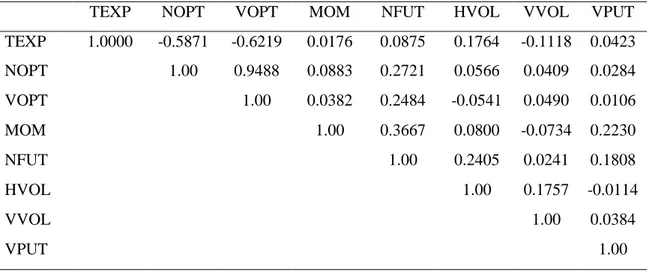
In Table II the results of correlation analysis between explanatory variables are presented. The high correlation coefficient between the two measures of transaction volume in the option market suggests to drop one of them; I decide to keep the variable “number of contracts”. The magnitude of the other correlation coefficients allows to maintain the other explanatory variables in the subsequent analysis.
In order to assess the stationarity of the employed variables, which is a crucial point, as we will see, in the application of the methodology of this paper, the first step is the calculation of the sample autocorrelation coefficients; as illustrated in Table III, the variables “historical volatility” and the “momentum” exhibit the most relevant degree of persistence. Given the importance of this issue, it is clear that a formal testing procedure is required to determine the order of integration. I conduct augmented Dickey Fuller tests, allowing for the possibility that the data-generation process contains a constant drift term and additional lagged terms for the dependent variables. The results, reported in the last column of Table III, suggest that indeed “historical volatility” and “momentum”14 can be integrated variables.
In order to get deeper understanding of the potential non stationarity of these time series, I follow the strategy proposed by Dolado et. al (1990) for testing for unit roots in the presence of possible trends. The procedure leads to the same previous results, that the existence of a unit root in “momentum” and “historical volatility” can not be rejected15. I conclude that these time
13 Bates (2000) shows graphically that the moneyness bias in the post-crash period is strongly related to a
percentage of out of the money call transactions on the total out of the money call and put transactions.
14 The coefficient for the variable “momentum” is very close to the boundary for the rejection of the null
hypothesis; since the true data-generating process is unknown and hence the test can potentially be misspecified, I do not reject the hypothesis of a unit root for “momentum” variable.
15 Similar results are obtained if the logarithm of historical volatility is employed instead of the original
series are integrated of order one, since the same tests on the first differences reject definitely the presence of a unit root.
3.
The implied volatility function
In this section the data are analysed in order to get a formal description of the empirical implied volatility function.
3.1
The pattern in the data
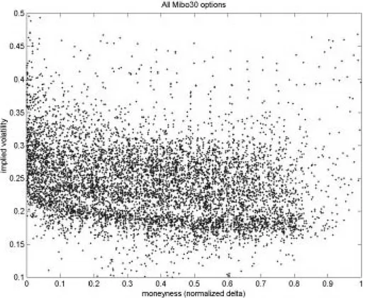
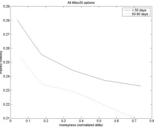
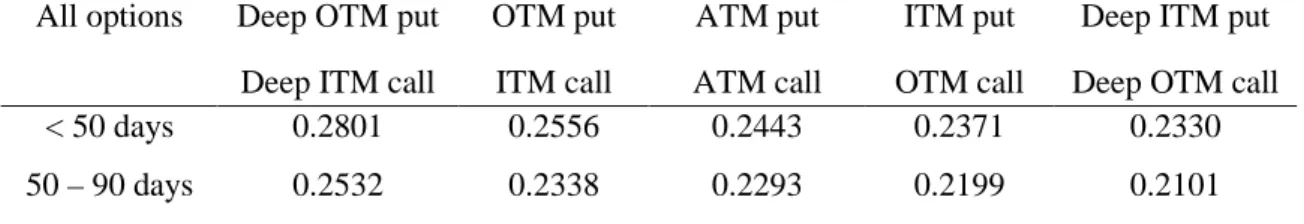
In order to determine the kind of model which could best fit option’s implied volatility with respect to option’s moneyness, it is useful to present a graphical plot of the data (see Figure 1). However, owing to the time varying general level of volatility, the picture is not so clear. Hence the option data is divided into several categories, according to either moneyness or time to expiration. By moneyness an option contract can be classified as: deep out of (in) the money put (call), out of (in) the money put (call), at the money put (call), in (out of) the money put (call), deep in (out of) the money put (call); the boundaries of the categories are chosen in order to have the same number of observations in each class16. By the time to expiration options are grouped in a short term category (<50 days) and medium term category (50-90 days). The proposed moneyness and maturity classification generates 12 categories; I equally weigh the implied volatility of each option in a given category to produce an average implied volatility per class. The results are summarized in Table IV and plotted in Figure 2.
The average implied volatility function presents the characteristic asymmetric profile (smirk): regardless the time to expiration, the Black’s implied volatility exhibits a strong decreasing pattern as the put option goes from deep out of the money, to at the money and then deep in the money or as the call goes from deep in the money, to at the money and then deep out of the money. Furthermore the different level of Black’s implied volatility between short and medium term options suggests the presence of a term structure of implied volatility.
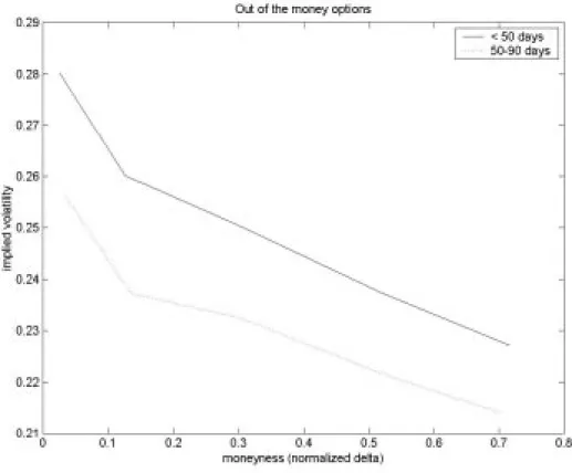
To avoid possible misspecifications due to illiquid prices or unexploited arbitrage opportunities, the same graphical analysis is performed using only out of the money call and put options, which are traded more frequently and are not suitable for some arbitrage strategies. The results are fairly the same: the smirk presents only a smoother profile (see Table V and Figure 3). I also
16 This choice depends on the descriptive purpose of this section; hence the focus is not on the precise
meaning of moneyness, for which I should set typical moneyness intervals, but rather on a reliable representation of implied volatility in each specified category.
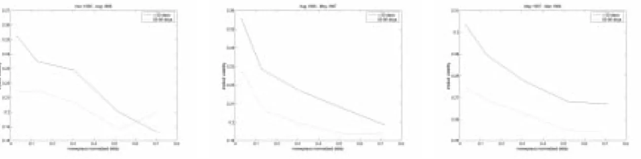
verify the persistency of this pattern throughout the period considered in this analysis. The breaking up in three sub-periods of about nine months17 shows that the implied volatility function is always characterized by an asymmetric smile, with a smoother profile in the latest period (see figure 4). Looking at the differences in y-axis values, the plot provides also an empirical evidence of the time varying general level of implied volatility.
These findings of clear moneyness-related and maturity related biases are consistent with those in the existing literature; the evidence of a steeper smile for short term options reported in the literature depends on a measure of moneyness which doesn’t take into account option’s time to expiration (e.g. the ratio between the strike price and the future price), as pointed out also in Dumas et. al (1998). Actually almost the same pattern for the implied volatility function is obtained using the other typical measures of options’ moneyness instead of options’ Delta, except for a steeper smile for short term options when moneyness measure is time independent18.
3.2
Model’s estimation
The shape of implied volatility function suggests to fit the data with the typical linear and quadratic model used previously in the literature (see Shimko (1993) or Dumas et al. (1998))19:
Model 1:
Y
=
β
0+
β
1X
+
ε
Model 2:
Y
=
β
0+
β
1X
+
β
2X
2+
ε
where Y, the dependent variable, represents the implied volatility and X the moneyness of the options. The simplicity of the two models is determined by the endeavour to avoid overparametrization in order to gain better estimates’ stability over time; moreover some other techniques, such as kernel regression (Ait-Sahalia (1998)), are not suitable in this study, because in that case the model is estimated only once on the whole dataset.
Specifically the time to maturity is not used in the models as one of the independent variables, owing to the lack of explanatory power and to the potential source of overfitting showed in the literature (e.g. Dumas et al. (1998)); anyway time to maturity is considered in the reminder of this analysis as one of the potential determinants of the specific profile of the implied volatility
17
The first sub-period is between 15.11.1995 and 21.08.1996, the second sub-period is between 22.08.1996 and 28.05.1997, the third is between 29.05.1997 and 03.03.1998.
18
To save space I do not insert the alternative plots and tables in this paper.
19 For the important analogies between the deterministic volatility function that I will use in this approach
and the implied binomial tree approach of Rubinstein (1994) or Derman and Kani (1994), see again Dumas et al. (1998).
function. Moreover I decide to give the same weight to each observation, regardless the moneyness, as the strategy to assign less weight to the deep out of the money options owing to the higher volatility has not proven to be satisfactory ( see Jackwerth and Rubinstein (1996)). However these models can hardly be estimated on the given dataset, because the general level of volatility is time-varying, as the plot of figure 1 easily shows20.
There are two possible procedures to neutralize the non-stationarity of volatility. First, the implied volatility can be standardized with respect to the daily level of at the money volatility, like in Tompkins (1999); the ratio between the actual level of implied volatility and at the money volatility of the same trading day turns out to be a stationary time series. However using this approach can lose, in a further analysis of the model, the potential effect of the level of volatility on the shape of the implied volatility function.
The second possible approach, that actually is employed in this study, is to fit the models separately on every trading day with sufficient observations; I implicitly assume that implied volatility is stationary during the day. Then, in order to obtain representative models’ parameters for the whole period, the average of the daily estimates is computed. I don’t need any at the money implied volatility estimate and information about the general level of volatility is retained.
Hence the models can slightly be rearranged to consider this approach:
Model 1:
Y
t,τ=
β
0+
β
1X
t,τ+
ε
t,τ∀
t
∈
(
0
,
T
]
,
∀
τ
∈
[ ]
5
,
90
Model 2:Y
t,τ=
β
0+
β
1X
t,τ+
β
2X
t2,τ+
ε
t,τ∀
t
∈
(
0
,
T
]
,
∀
τ
∈
[ ]
5
,
90
where Y represents implied volatility and X the moneyness expressed as the normalized Delta measure21, while t denotes trading days and τ options’ time to maturity. A single model is estimated for each trading day considering options with the same time to maturity; typically two models are estimated for each trading day.
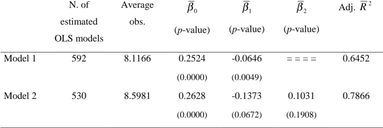
The results obtained by OLS fitting procedure are shown in Table VI. The reported parameters’ estimates are averages for the whole period and so it is for the adjusted R2. The t-statistics on which the p-values are computed use the average value of the parameter and average standard error, instead of averaging the t-values of each model22.
20 Trying to fit Model 1 on the raw dataset returns an R2 of 0.07. 21
The results are similar when different measures of moneyness are employed.
22 This approach to hypothesis testing in presence of aggregation problems is used also in the literature on
“event-study analysis” when cumulative abnormal return observations are evaluated. For a comprehensive reference see Campbell, Lo and MacKinlay (1997 p. 160-163).
The differences between Model 1 and Model 2 in the number of OLS estimations and in the average number of observations used in each inference are explained obviously by the higher observations requirement of Model 2 with respect to Model 1. The economic interpretation of the values obtained for the parameters is straightforward:
β
0 represents a general level of volatility which localizes the implied volatility function,β
1 characterizes the negative profilewhich is responsible for the asymmetry in the risk neutral probability density function and
β
2 provides, in Model 2, a certain degree of curvature in the implied volatility function. Hence the average risk neutral PDF on the Italian stock market is fat tailed and negatively skewed.From the analysis of the p-values reported in Table VI, all the estimated parameters but
β
2 can be considered significant. This can cast some doubts on the opportunity to use Model 2 in the reminder of the analysis, even though the adjusted R2 exhibits a substantial difference. For this reason a Lagrange Multiplier (LM) statistic is performed to test whether the coefficient associated with the quadratic term is statistically different from zero; the restricted model turns out to be Model 1 and the LM test is asymptotically distributed as a chi-squared with one degree of freedom. The value obtained for the LM statistic is 528.91 (p-value 0.0000); this implies that the null hypothesis ofβ
2 equal to zero is rejected and hence Model 2 is employed in thesubsequent part of this study.
4.
Identifying the potential determinants
In the previous section it was shown that the average implied volatility function is fitted rather well by a quadratic model with a negative coefficient of asymmetry.
In order to identify which explanatory variables can potentially determine the observed profile of the implied volatility smile, a linear and non-linear Granger Causality test is performed between the estimated parameters of Model 2 and the potential determinants described in Section 2. I will try to find a relation between the degree of asymmetry (β1), the degree of
curvature (β2) and seven explanatory variables. In some sense the contract specific variables
should help to detect cross sectional pricing biases, whereas the other variables serve to indicate whether the smile profile over time, which means the Black and Scholes pricing error, is related to the dynamically changing market conditions.
4.1
Linear Granger Causality
In this paragraph I discuss the definition of Granger causality and the basic approach used to test for its presence. Because this approach is well known, only a brief discussion is offered here.
As originally specified, the general formalization of Granger (1969) causality for the case of two scalar valued, stationary time series { Xt } and { Yt } is defined as follows. Let F
(
XtYt−1)
be the conditional probability distribution of Xt given the bivariate information set It-1 of an
lx-length lagged vector of Xt , say Xtt−−1lx ≡
(
Xt−lx,Xt−lx+1,...,Xt−1)
, and an ly-length lagged vector ofYt , say Ytt−−ly1≡
(
Yt−ly,Yt−ly+1,...,Yt−1)
. Given lags lx and ly , the time series { Yt } does not strictlyGranger cause { Xt } if:
(
)
(
1)
1 1 − − − −=
t t−
ttly t tI
F
X
I
Y
X
F
t = 1,2,…. (1)If the equality in equation (1) does not hold, then knowledge of past Y values helps to predict current and future X values, and Y is said to strictly Granger cause X. Similarly, a lack of instantaneous Granger causality form Y to X occurs if:
(
X
tI
t) (
F
X
tI
tY
t)
F
−1=
−1+
(2)where the bivariate information set is modified to include the current value of Y. If the equality in equation (2) does not hold, then Y is said to instantaneously Granger cause X.
Strict Granger causality relates to the past of one time series influencing the present and future of another time series, whereas instantaneous causality refers to the present of one time series influencing the present of another time series23.
The well-known test for Granger causality involves the estimation of a linear reduced form vector autoregression (VAR):
t kt it it t kt it it
u
E
L
B
L
B
E
u
E
L
B
L
B
, 2 22 21 2 , 1 12 11 1)
(
)
(
)
(
)
(
+
+
+
=
+
+
+
=
β
α
β
α
β
(3)for t=1,2,… i=1,2 and k=1,…,7
where βit is alternatively the coefficient of asymmetry or the degree of curvature, Ekt is a single
explanatory variable, B11(L), B12(L), B21(L) and B22(L) are one sided lag polynomials in the lag
23 See Geweke, Meese and Dent (1983), Granger and Newbold (1986) and Hendry and Mizon (1999) for
a discussion of Granger causality testing procedures and issues relative to omitted variables bias, measurement errors and aggregation bias.
operator L. The regression errors {u1,t} and {u2,t} are assumed to be mutually independent and
individually i.i.d. with zero mean and constant variance.
To test for strict Granger causality from Y to X a standard joint test (F- or χ2 – test) of exclusion restriction is used to determine whether lagged Y has significant linear predictive power for current X. The null hypothesis that Y does not strictly Granger cause X is rejected if the coefficients on the elements in B12(L), i.e. B12,i (i=1,..,m) are jointly significantly different from
zero. Feedback (or bi-directional) causality exists if Granger causality runs in both directions, in which case the coefficients on the elements in both B12(L), B21(L) are jointly different from
zero.
Among the variety of causality tests that have been proposed, the simplest and straightforward approach uses an autoregressive specification24. To implement this test, I assume a particular lag length L and estimate by OLS :
t L kt L kt kt L it L it it it
=
α
1+
b
1β
−1+
b
2β
−2+
...
+
b
β
−+
c
1E
−1+
c
2E
−2+
...
+
c
E
−+
u
β
(4) t L it L it it it=
α
+
d
β
−+
d
β
−+
+
d
β
−+
e
β
2 1 1 2 2...
(5)I compute the sum of squared residuals from (4) and (5),
∑
==
T t tu
RSS
1 2 1ˆ
∑
==
T t te
RSS
1 2 0ˆ
if(
)
1 1 0 1RSS
RSS
RSS
T
S
=
−
is greater than the 5% critical value for a χ2(L) variable, then the null hypothesis that E does not
Granger-cause β is rejected; that is, if S1 is sufficiently large, I conclude that E does
Granger-cause β.
4.2
Nonlinear Granger Causality
Baek and Brock (1992) proposed a nonparametric statistical method for detecting nonlinear causal relations between two time series. This method was modified by Hiemstra and Jones (1994) to allow each series to display weak temporal dependence. To define nonlinear Granger
24 Based on Monte Carlo simulations, Geweke, Meese and Dent (1983) suggest that the causality test I am
causality, assume there are two strictly stationary and weakly dependent scalar time series {Wt }
and {Vt }. As in the previous paragraph, define the m-length lead vector of Wt by Wt m
, and the Lw-length and Lv-length lag vectors of Wt and Vt , respectively, by Wtm ≡
(
Wt,Wt+1,...,Wt+m−1)
(
− , − +1,..., −1)
− ≡ tlw t lw t lw lw t W W W W and −lv ≡(
t−lv, t−lv+1,..., t−1)
lv t V V V V .The definition of nonlinear Granger noncausality is given by Eq. (6):
(
)
(
W
W
e
W
W
e
)
e
V
V
e
W
W
e
W
W
Lw Lw s Lw Lw t m s m t Lv Lv s Lv Lv t Lw Lw s Lw Lw t m s m t<
−
<
−
=
<
−
<
−
<
−
− − − − − −Pr
,
Pr
(6)where Pr{.} denotes probability and is the maximum norm. If Eq. (6) holds, for given values of m, Lw, and Lv and for e, then {Vt} does not strictly Granger cause {Wt}. This
definition of nonlinear Granger causality is based on two conditional probabilities. The probability on the left hand side of Eq. (6) can be interpreted as the conditional probability that any two arbitrary m-length lead vectors of {Wt} are within a metric e of each other, given that
the corresponding Lw-length lag vectors of {Wt} and Lv-length lag vectors of {Vt} are within a
distance e of each other. The probability on the right hand side of Eq. (6) can be interpreted in a similar way: the conditional probability that any two arbitrary m-length lead vectors of {Wt} are
within a metric e of each other, given that the corresponding Lw-length lag vectors of {Wt} are
within a distance e of each other. The null hypothesis is that {Vt} does not nonlinearly Granger
cause {Wt}. Under the null hypothesis, and for given values of m, Lw and Lv ≥ 1and e >0, it can
be shown that the statistic:
(
)
(
)
C
(
(
Lw
e
n
)
)
aN
(
(
m
Lx
Ly
e
)
)
n
e
Lw
m
C
n
e
Lv
Lw
C
n
e
Lv
Lw
m
C
n
~
0
,
,
,
,
,
,
4
,
,
3
,
,
,
2
,
,
,
1
σ
2
+
−
+
(7)where C1(m+Lw, Lv, e, n), C2(Lw, Lv, e, n), C3(m+Lw, e, n), and C4(Lw, e, n) are correlation-integral estimators of the point probabilities corresponding to the left hand side and right hand side of Eq. (6)25. This test has very good power properties against a variety of nonlinear Granger causal and noncausal relations, and its asymptotic distribution is the same if the test is applied to the estimated residuals from a vector autoregressive (VAR) model (Hiemstra and Jones (1994)).
25 For a more detailed discussion of correlation integral estimators and the derivation of the estimator for
4.3
Linear Granger test results
Since hypothesis tests are sensitive to the truncation of the lag polynomials on the dependent and independent variable, lag lengths must be chosen carefully26. In order to determine the optimal lag, two of the typical information criteria: Akaike Information Criteria and Schwarz Information Criteria are employed that share the common aim to trade off the bias associated with a parsimonious parametrization against the inefficiency associated with overparametrization. In the few cases in which the suggested optimal lag is not the same, I follow the Schwarz result that seems to be more parsimonious and stable.
A second issue is related to the non stationary of the variables employed in this analysis; in Section 2.4 it was shown that the variables “momentum” and “historical volatility” are integrated of order one ( I(1) ), so that first differences are individually stationary and hence suitable for modelling in a Vector AutoRegression framework. However Engle and Granger (1987) show that if two nonstationary variables are cointegrated, a VAR in the first differences is misspecified. For two series of prices to be cointegrated, each one must be I(1) and there exists a linear combination which is stationary. As in the employed model one of the dependent variables is always a parameter of the implied volatility function, β1 or β2 , first of all the order
of integration of these series of parameters is determined. Applying the same augmented Dickey Fuller test of Section 2.4, I find that each series is I(0) or, in other words, is stationary. This means that the presence of cointegration is always rejected and the VAR model in the differences is correctly specified.
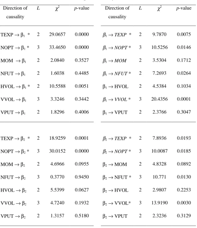
Table VII reports the results of the linear Granger causality tests between the asymmetry parameter β1 and the explanatory variables and between the curvature parameter β2 and the
explanatory variables27. Beside the optimal lag determined by the usual information criteria, the value of chi-squared statistic and the correspondent p-value is indicated.
The first evidence is the prominent role played by the time to expiration variable. This is consistent with findings in the literature about the presence of a term structure of implied volatility and hence confirms that Black and Scholes pricing errors are different for options with different expiration dates. This effect is apparent even if Delta has been employed as a measure
26
For a discussion and statistical comparison of alternative techniques to set lag lengths while conducting causality tests, see Thornton and Batten (1985).
27 I do not report in the tables the results of linear causality between the intercept of the model β
0 and the
explanatory variables; in fact an economic interpretation of β0 as a proxy for the general level of implied
volatility can be misleading and is not particularly useful for the implications of this paper. Only for the sake of completeness, I found that each of the employed potential determinants significantly causes β0,
except momentum, volatility of volatility and the percentage of out of the money put options on the total of transacted options.
of moneyness, neutralizing in this way a typical moneyness misspecification. The effect of option’s time to expiration is evident both on the asymmetry and on the curvature parameter, hence influencing both skewness and kurtosis of the implied risk neutral PDF.
A second evidence can be inferred by the results obtained for the variable “number of option contracts”; a liquidity story seems to apply also in the relative mispricing of Black and Scholes model with respect to moneyness. This result is even more significant than previous findings relative to the bid-ask spread (e.g. Pena et. al (1999)); in fact this measure is not related directly with moneyness and hence is not subject to the chance of being significant simply because it is picking up part of the moneyness effect28. Both time to expiration and number of contracts show significant feedback effect from the correspondent smile coefficient: hence bi-directional Granger causality is ascertained.
The historical volatility of the underlying is found to be significant in determining the asymmetry parameter β1; this evidence provides further matter for the adoption of pricing model
with stochastic volatility and of models estimated exploiting jointly the dynamics of options prices and underlying asset (e.g. Pan, 2000).
The fact that the variable VPUT, which is the ratio between out of the money put options on total transacted options, does not Granger cause the profile of the smile could be consistent with the problems in finding reliable proxies of the portfolio insurance activity of fund managers; in fact this activity is usually carried out over the counter, owing to big amounts involved and needs of longer maturities. This could also be consistent with a limited portfolio insurance activity carried out by Italian fund managers during the period under analysis.
The other potential explanatory variables are not found to significantly cause the asymmetry and curvature of the volatility smile.
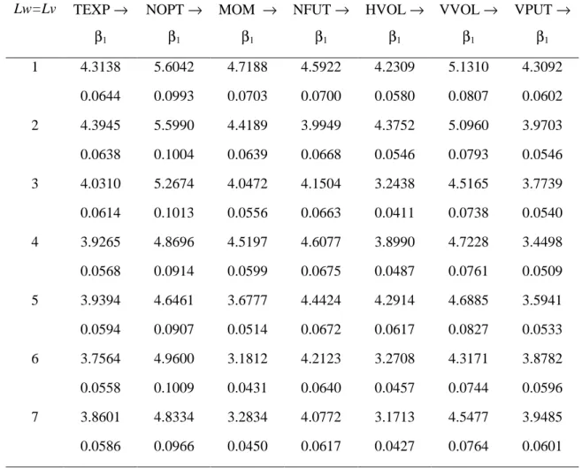
4.4
Modified Baek and Brock test results
In this paper the modified Baek and Brock test is applied on the estimated residuals from Eq. (3) (i.e. {u1,t} and {u2,t}) and not on the original series. The estimated residuals do not contain any
linear causality structure since they are filtered series obtained from the VARs.
The next step, before applying the modified Baek and Brock test, is to establish the value for the lead length m, the lag lengths Lw and Lv and the scale parameter e. Unlike linear causality
28 Bakshi et al. (1997) show that in a regression of percentage pricing error on some explanatory
variables, the coefficient for the bid-ask spread is of high magnitude for Black e Scholes model and of lower magnitude for a simple stochastic volatility models; a possible explanation is that the bid-ask spread is actually picking up part of the moneyness effect.
testing, there is no literature on the appropriate way to specify these values optimally. On the basis of the Monte Carlo tests cited in Hiemstra and Jones (1994), I set for all cases, m=1 using common lag lengths of 1 to 7 lags. Moreover, for all cases, the test is applied to standardized series, using the scale parameter e =1.5σ , where σ =1 denotes the standard deviation of the
standardized time series; in conducting the test similar results are obtained using scale parameter values of 1.0σ and 0.5σ.
The results from nonlinear Granger causality testing between the parameter β1 and the seven
explanatory variables are reported in Table VIII. A significant nonlinear causality relation is found for each variable; these results are robust to changes in the employed lag. Moreover all the explanatory variables seem also to nonlinearly Granger cause the curvature parameter β2 ,
even if this evidence is slightly less significant. The nonlinear inverse causality is rejected for both β1 and β2 when the explanatory variable is the time to expiration, the historical volatility or
the momentum.
The straightforward interpretation of these results is that the dynamic relation between the implied volatility function and variables related to the underlying, to investor behaviour or to the options market itself is to some extent nonlinear. This finding may suggest that future research should consider nonlinear theoretical mechanism when developing or assessing models of options’ pricing or joint dynamics between true and risk neutral processes.
5.
Conclusions
This study analyses the potential determinants of the volatility smile, i.e. the well known pattern of implied volatilities with respect to moneyness. The employed database is comprised by daily closing prices of call and put options on Mib30 Italian stock index from November 1995 to March 1998. I find that the Italian stock market tends to show a rather straight decreasing profile consistently throughout the sample period, similarly to the US market; this pattern is well interpreted by a simple quadratic model of implied volatility in moneyness.
Linear and nonlinear Granger causality test are performed in order to find potential explanatory variables of the observed pattern of implied volatilities. The results show a linear causal relation of the time to expiration, the number of transacted option contracts and historical volatility on the asymmetry of the smile profile; this evidence confirms both the importance of the term structure of implied volatility on Black and Scholes mispricings, the role of market liquidity and the requirement of stochastic volatility in any option pricing model. The findings of the
nonlinear Granger causality tests suggest that for the other explanatory variables the effect on the implied volatility function could be nonlinear.
Although the linear and nonlinear approach of causality testing presented in this paper can detect causal dependence with high power, it provides no guidance regarding the source of this dependence. Such guidance should be left to theory, which may propose specific models. However the results of this paper suggest that these models ought to deal with at least time to expiration and stochastic volatility. As this doesn’t seem to be sufficient to explain Black and Scholes biases, as Bakshi et al. (1997) and Bates (2000) show, a promising way to take in to account some of the other dependencies found in the present study could be to analyse jointly the dynamics of the true and risk neutral process. In particular the introduction of risk premiums (see Pan, 2000) can explain some puzzling evidence.
References
Aït-Sahalia, Y. and A.W. Lo (1998), “Nonparametric Estimation of State-Price Densities Implicit in Financial Asset Prices”, in Journal of Finance, vol. 53, nr. 2, April, pp. 499-548. Baek E., and W. Brock (1992), “A general test for nonlinear Granger causality: Bivariate model”, Working paper, Iowa State University University Wisconsin Madison.
Bakshi, G., C. Cao and Z. Chen (1997), “Empirical Performance of Alternative Option Pricing Models”, in Journal of Finance, vol. 52, no. 5, December, pp. 2003-2049.
Bates, D. (1996), “Jumps and Stochastic Volatility: Exchange Rate Processes Implicit in DeutscheMark Options”, in Review of Financial Studies, vol. 9 Spring pp.69-107.
Bates, D. (2000), “Post-’87 crash fears in the S&P 500 futures option market”, in Journal of
Econometrics, vol. 94 pp. 181-238.
Black, F. (1976), “The Pricing of Commodity Contracts”, in Journal of Financial Economics, vol. 3, nr. 3, pp. 167-179.
Black, F. and M. Scholes (1973), “The Pricing of Options and Corporate Liabilities”, in Journal
of Political Economy, vol. 81, May-June, pp. 637-654.
Campbell J.Y., A.W. Lo and A.C. MacKinlay (1997), The Econometrics of Financial Markets, Princeton University Press, Princeton, New Jersey.
Derman, E. and I. Kani (1994), “Riding on a Smile”, in Risk, vol. 7, nr. 2, February, pp.32-39. Dolado, J.J., T. Jenkinson and S. Sosvilla-Rivero (1990), “Cointegration and Unit Roots”, in
Journal of Economic Surveys, 4, pp. 249-273.
Dumas, B., J. Fleming and R.E. Whaley (1998), “Implied Volatility Functions: Empirical Tests”, in Journal of Finance, vol. 53, nr. 6, December, pp. 2059-2106.
Engle, R. and C. Granger (1987), “Co-Integration and Error Correction: Representation, Estimation, Testing”, in Econometrica, 55, pp. 251-276.
Gallant A.R., P. E. Rossi and G. Tauchen (1992), “Stock Prices and Volume”, in Review of
Financial Studies, vol. 5, pp. 199-242.
Geweke J., R. Meese and W. Dent (1983), “Comparing alternative tests of causality in temporal systems”, in Journal of Econometrics, vol. 21, pp. 161-194.
Granger, C. (1969), “Investigating causal relations by econometric models and cross-spectral methods, in Econometrica, vol. 37, pp. 424-438.
Granger, C. and P. Newbold (1986), Forecasting economic time series, Academic Press Inc. 2nd ed., San Diego.
Greene, W.H. (2000), Econometric Analysis, Upper Saddle River, New Jersey, Prentice-Hall. Grossman S.J. and Z. Zhou (1996), “Equilibrium Analysis of Portfolio Insurance”, in Journal of
Finance, vol. 51 nr. 4, September, pp. 1379-1403.
Fuller, W. A. (1976), Introduction to Statistical Time Series, Wiley, New York, New York. Hamilton, J.D. (1994), Time Series Analysis, Princeton University Press, Princeton, New Jersey. Hendry D.F. and G.E. Mizon (1999), The Pervasiveness of Granger Causality in Econometrics, in Engle R. and H. White (editors), Cointegration, Causality and Forecasting: A Festschrift in Honour of Clive W.J. Granger, Oxford University Press, Oxford, New York.
Hentschel, L. (2000), “Errors in Implied Volatility Estimation”, Working Paper, Simon School, University of Rochester.
Heston, S. (1993), “A Closed-Form Solution for Options with Stochastic Volatility with Applications to Bond and Currency Options” in Review of Financial Studies, vol. 6 nr. 2, pp. 327-343.
Hiemstra C. and J. D. Jones (1994), “Testing for linear and nonlinear Granger causality in the stock price-volume relation” , in Journal of Finance, vol. 49, pp. 1639-1664.
Hull, J. and A. White (1987), “The Pricing of Options on Assets with Stochastic Volatilities” in
Journal of Finance, vol. 42, pp.281-300.
Jackwerth, J.C. (1999), “Option-implied Risk-neutral Distributions and Implied Binomial Trees: A Literature Review”, in Journal of Derivatives 7, No. 2, pp. 66-82.
Jackwerth, J.C. and M. Rubinstein (1996), “Recovering Probability Distributions from Option Prices”, in Journal of Finance, vol. 51, pp. 1611-1631.
Natenberg, S. (1994), Option Volatility and Pricing: Advanced Trading Strategies and Techniques, Probus Publishing, Chicago, Illinois.
Pan, J. (2000), “Integrated Time-Series Analysis of Spot and Option Prices”, Working Paper, MIT.
Pena, I., G. Rubio, G. Serna (1999), “Why do we smile? On the determinants of the implied volatility function”, in Journal of Banking & Finance, vol. 23, pp. 1151-1179.
Platen, E., Schweitzer, M. (1998), “On feedback effects from hedging derivatives”, in
Mathematical Finance, vol. 8, pp. 67-84.
Rubinstein, M. (1994), “Implied Binomial Trees”, in Journal of Finance, vol. 49, nr. 3, July, pp. 771-818.
Schwert, G. W. (1989), “Why Does Stock Market Volatility Change Over Time?”, in Journal of
Finance, vol. 44, pp. 1115-1153.
Shimko, D. (1993), “Bounds of Probability”, in Risk, vol.6, nr. 4, April, pp. 33-37.
Thornton D. and D. Batten (1985), “Lag-Length Selection and Tests of Granger Causality Between Money and Income”, in Journal of Money, Credit and Banking, vol. 17, pp. 164-178. Tompkins, R.G. (1999), Implied Volatility Surfaces: Uncovering Regularities for Options on Financial Futures, Working Paper No. 49, University of Vienna.
Figures
Figure 2: Average implied volatilities for classes of moneyness-time to expiration.
In order to have the same number of observations in each of the 5 moneyness’ classes I determine the following intervals: 0-0.092; 0.092-0.264; 0.264-0.438; 0.438-0.623; 0.623-1.
Figure 3: Average implied volatilities of out of the money options.
Also in this case, in order to have the same number of observations in each of the 5 moneyness’ classes, I have determined the following intervals: 0-0.061; 0.061-0.206; 0.206-0.405; 0.405-0.627; 0.627-1.
Figure 4: Implied volatility functions of out of the money options in three sub-periods.
The intervals of moneyness’ classes are the following: for the first sub-period 0-0.072; 0.072-0.21; 0.21-0.414; 0.414-0.624; 0.624-1. For the second sub-period 0-0.075; 0.075-0.22; 0.22-0.438; 0.438-0.669; 0.669-1. For the third sub-period 0-0.046; 0.046-0.19; 0.19-0.379; 0.379-0.607; 0.607-1.
The first sub-period is between 15.11.1995 and 21.08.1996, the second sub-period is between 22.08.1996 and 28.05.1997, the third is between 29.05.1997 and 03.03.1998.
Tables
Table I
Summary Statistics for Mib30 Index Options Data
Percentiles
Variable Mean Std. D Min. 5% 10% 50% 90% 95% Max
Implied σ (%) 24.20 5.59 10.03 16.62 17.70 23.70 31.03 33.89 49.54 Implied ATM σ 23.65 4.53 14.77 17.30 18.52 22.78 29.76 31.42 41.85 τ (trading days) 40.92 21.24 5.00 10.00 14.00 39.00 71.00 80.00 90.00 K (index points) 19049.84 4401.11 12500 13500 14000 18500 25000 27500 31500 F (index points) 18304.03 4181.79 13484 14028 14234 16268 24122 27091 29913 r (%) 8.11 1.36 6.13 6.25 6.69 7.56 10.13 10.56 10.81
Summary statistics for the filtered sample of traded Mibo30 daily call and put option prices on the Mib30
index in the period November 15, 1995 to March 3, 1998 (7.963 observations). “Implied σ ” denotes the
implied volatility of the option, and “Implied ATM σ ” denotes the implied volatility of at the money
options. τ denotes the options time to expiration, r the riskless rate, K the options strike price and F the Fib30 stock index future value. “Std. D.” denotes the sample standard deviation of the variable.
Table II
Correlation coefficients between explanatory variables
TEXP NOPT VOPT MOM NFUT HVOL VVOL VPUT
TEXP 1.0000 -0.5871 -0.6219 0.0176 0.0875 0.1764 -0.1118 0.0423 NOPT 1.00 0.9488 0.0883 0.2721 0.0566 0.0409 0.0284 VOPT 1.00 0.0382 0.2484 -0.0541 0.0490 0.0106 MOM 1.00 0.3667 0.0800 -0.0734 0.2230 NFUT 1.00 0.2405 0.0241 0.1808 HVOL 1.00 0.1757 -0.0114 VVOL 1.00 0.0384 VPUT 1.00
Correlation coefficients between the explanatory variables in the same period of options’ observations (November 15, 1995 to March 3, 1998). These variables are labelled and defined as in Section 2.3.
Table III
Descriptive statistics of explanatory variables
Mean Std. Dev. ρ (1) ρ (5) ρ (10) ADF
TEXP 41.9415 20.7454 0.9219 0.6358 0.3666 -4.5234* NOPT 823.3981 1013.5480 0.6523 0.4942 0.2295 -7.3852* MOM 0.0346 0.0566 0.9558 0.7758 0.5393 -3.5118* NFUT 14217.93 5822.566 0.6738 0.3944 0.3454 -7.8913* HVOL 0.2099 0.0616 0.9664 0.8070 0.6019 -3.3988 VVOL 0.0279 0.0175 0.9396 0.5632 0.1925 -4.3541* VPUT 0.5517 0.2037 0.1701 0.1553 0.1443 -11.9977*
Descriptive statistics for the explanatory variables in the same period of options’ observations (November 15, 1995 to March 3, 1998). “Mean” denotes the sample mean of the variable, “Std. Dev.” denotes the
sample standard deviation of the variable and “ρ (k)” denotes the sample autocorrelation coefficient at lag
k of the variable. “ADF” denotes the value for the augmented Dickey Fuller test; the star represents the
cases in which the null hypothesis of a unit root is rejected at the 0.99 confidence level (the empirical cumulative distribution for this test is reported in Fuller (1976)).
Table IV
Implied volatility per classes of moneyness/time to expiration
All options Deep OTM put Deep ITM call
OTM put ITM call ATM put ATM call ITM put OTM call
Deep ITM put Deep OTM call
< 50 days 0.2801 0.2556 0.2443 0.2371 0.2330
50 – 90 days 0.2532 0.2338 0.2293 0.2199 0.2101
I represent an average implied volatility for each category obtained by equally weighting each observation. The moneyness intervals, chosen to have the same number of observations in each class, are the following (expressed as a normalized Delta): 0-0.092; 0.092-0.264; 0.264-0.438; 0.438-0.623; 0.623-1.
Table V
Implied volatility per classes of moneyness/time to expiration
OTM options Deep OTM
put
OTM put ATM put OTM call Deep OTM
call
< 50 days 0.2802 0.2601 0.2502 0.2373 0.2272
50 – 90 days 0.2561 0.2373 0.2325 0.2214 0.2140
I represent an average implied volatility for each category obtained by equally weighting each observation, but considering only out of the money options. The moneyness intervals, chosen to have the same number of observations in each class, are the following (expressed as a normalized Delta): 0-0.061; 0.061-0.206; 0.206-0.405; 0.405-0.627; 0.627-1. Notice that the process of normalization allows to have on the same axis both out of the money call and put options, with the moneyness increasing with the strike price.
Table VI
Model estimation statistics
N. of estimated OLS models Average obs. 0
β
(p-value) 1β
(p-value) 2β
(p-value) Adj.R
2 Model 1 592 8.1166 0.2524 -0.0646 = = = = 0.6452 (0.0000) (0.0049) Model 2 530 8.5981 0.2628 -0.1373 0.1031 0.7866 (0.0000) (0.0672) (0.1908)The “N. of estimated OLS models” refers to the number of implied volatility function estimated each day for options with the same expiration. “Average obs.” denotes the average number of observations available in each implied volatility smile estimation. The numbers in parentheses are the p-values of the
correspondent average β coefficients for the t-statistics. The adjusted R2 accounts for the degree of freedoms and is computed as an average of the adjusted R2 coefficient in each model.