DIPARTIMENTO DI INGEGNERIA INDUSTRIALE E SCIENZE MATEMATICHE
-DIISM
Corso di Dottorato di Ricerca in Ingegneria Industriale – Curriculum Ingegneria Energetica
Ph.D. Thesis
Experimental and numerical analysis of natural
convection in a square cavity with a vertical baffle
Advisor:
Prof. Corvaro Francesco
Curriculum Supervisor:
Prof. Ferruccio Mandorli
Ph.D. Dissertation of:
Benucci Maurizio
1 Overview of natural convection in cavity 1
1.1 General concept of natural convection . . . 1
1.2 Square and rectangular cavity with internal baffle . . . 3
1.3 Variables affecting natural convection in cavity . . . 6
2 Materials and methods 9 2.1 Experimental technique . . . 9
2.1.1 PIV set-up . . . 9
2.1.2 Measurement procedure . . . 13
2.1.3 Data analysis . . . 15
2.1.4 Two-dimensionality of the flow . . . 19
2.1.5 PIV measurements convergence . . . 19
2.2 Numerical technique . . . 21
2.2.1 Geometry and mesh . . . 23
2.2.2 Pure convection model . . . 25
2.2.3 Combined Convective-radiative model . . . 28
2.2.4 Data analysis . . . 29
2.2.5 Numerical accuracy . . . 29
3 Effects of the baffle height and position 31 3.1 Effect of the aperture ratio for a central baffle . . . 31
3.2 Effect of the baffle position . . . 41
4 Effect of the radiative heat transfer 59 5 Effect of the tilting angle 75 6 Conclusions 85 A Nomenclature 89 A.1 Latin Symbols . . . 89
A.2 Greek Symbols . . . 90
A.3 Subscripts . . . 91
A.4 Acronyms . . . 91
Bibliography 93
2.9 Output of the vector statistics algorithm. . . 18 2.10 Results of the experimental post-processing. . . 19 2.11 Average velocity profile at H/2 for Ap= 1/5, p = 3L/10 and Ra = 3.8×10⁵. 20
2.12 Average velocity profile at H/2 for Ap= 1/5, p = L/2 and Ra = 3.8 × 10⁵. 20
2.13 Average velocity profile at H/2 for Ap= 1/5, p = 7L/10 and Ra = 3.8×10⁵. 20
2.14 PIV realization convergence at H/2 and x/L = 0.1 for Ap = 1/5and
Ra= 3.8 × 10⁵. . . . 21
2.15 PIV realization convergence at H/2 and x/L = 0.9 for Ap = 1/5and
Ra= 3.8 × 10⁵. . . . 21
2.16 PIV realization convergence for Ra = 3.8 × 10⁵. . . . 22
2.17 Visualization of the differences between continuous and discrete domain. 23 2.18 Computational geometry. . . 24 2.19 Computational grid. . . 25 2.20 Average Nusselt number values by numerical simulation performed for
Ap= 1/5and Ra = 3.8 × 10⁵ with different grid sizes. . . 30
2.21 Maximum and average velocity values by numerical simulation performed for Ap= 1/5and Ra = 3.8 × 10⁵with different grid sizes. . . 30
3.1 Numerical scalar velocity maps for the baffle located at x/L = 1/2. . . 32 3.2 Numerical streamlines for the baffle located at x/L = 1/2. . . 33 3.3 Numerical isotherms for the baffle located at x/L = 1/2. . . 34 3.4 Experimental scalar velocity maps for the baffle located at x/L = 1/2. 36 3.5 Experimental streamlines for the baffle located at x/L = 1/2. . . 37 3.6 Maximum velocity for each case with the baffle located at x/L = 1/2. 38 3.7 Average velocity for each case with the baffle located at x/L = 1/2. . . 38 3.8 Local Nusselt number along with the vertical hot wall for an enclosure
with the baffle located at x/L = 1/2. . . 39 vi
correlations from Kirkpatrick [14] and Acharya and Jetli [17] . . . 41
3.10 Numerical isotherms for the baffle located at x/L = 3/10. . . 43
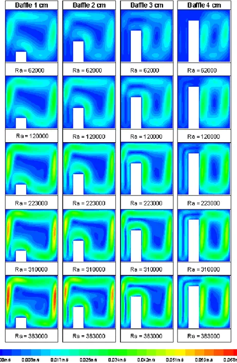
3.11 Numerical scalar velocity maps for the baffle located at x/L = 3/10. . 44
3.12 Numerical streamlines for the baffle located at x/L = 3/10. . . 45
3.13 Numerical isotherms for the baffle located at x/L = 7/10. . . 46
3.14 Numerical scalar velocity maps for the baffle located at x/L = 7/10. . 47
3.15 Numerical streamlines for the baffle located at x/L = 7/10. . . 48
3.16 Experimental scalar velocity maps for the baffle located at x/L = 3/10. 49 3.17 Experimental scalar velocity maps for the baffle located at x/L = 7/10. 50 3.18 Experimental streamlines for the baffle located at x/L = 3/10. . . 51
3.19 Experimental streamlines for the baffle located at x/L = 7/10. . . 52
3.20 Maximum velocity for each case with the baffle located at x/L = 3/10. 54 3.21 Average velocity for each case with the baffle located at x/L = 3/10. . 54
3.22 Maximum velocity for each case with the baffle located at x/L = 7/10. 55 3.23 Average velocity for each case with the baffle located at x/L = 7/10. . 55
3.24 Local Nusselt number along the vertical hot wall for an enclosure with the baffle located at x/L = 3/10. . . 56
3.25 Local Nusselt number along the vertical hot wall for an enclosure with the baffle located at x/L = 7/10. . . 57
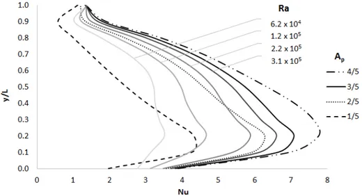
3.26 Average Nusselt number as a function of the Rayleigh number. . . 58
4.1 Numerical scalar velocity maps for the baffle located at x/L = 1/2. . . 60
4.2 Numerical scalar velocity maps for the baffle located at x/L = 3/10. . 61
4.3 Numerical scalar velocity maps for the baffle located at x/L = 7/10. . 62
4.4 Numerical streamlines for the baffle located at x/L = 1/2. . . 63
4.5 Numerical streamlines for the baffle located at x/L = 3/10. . . 64
4.6 Numerical streamlines for the baffle located at x/L = 7/10. . . 65
4.7 Numerical isotherms for the baffle located at x/L = 1/2. . . 66
4.8 Numerical isotherms for the baffle located at x/L = 3/10. . . 67
4.9 Numerical isotherms for the baffle located at x/L = 7/10. . . 68
4.10 Numerical (convective-radiative model) local Nusselt number along the vertical hot wall for an enclosure with the baffle located at x/L = 3/10. 71 4.11 Numerical (convective-radiative model) local Nusselt number along the vertical hot wall for an enclosure with the baffle located at x/L = 1/2. 72 4.12 Numerical (convective-radiative model) local Nusselt number along the vertical hot wall for an enclosure with the baffle located at x/L = 7/10. 74 4.13 Numerical average Nusselt number for the case with the baffle located at x/L = 1/2 and Ap= 2/5. Dotted line represents the pure convection results while the continuous lines show the different contribution of radiative, convective and overall heat transfer. . . 74
5.1 Numerical scalar velocity maps. . . 77
5.2 Numerical streamlines. . . 78
5.3 Numerical isotherms. . . 79
5.4 Experimental scalar velocity maps. . . 80
5.5 Experimental streamlines. . . 81
5.6 Numerical (pure convection model) local Nusselt number along the vertical hot wall for Ra = 3.8 × 10⁵. . . . 83
2.4 Standard deviation of repeated measurements for each case study. . . 15 2.5 Emissivity. . . 29 2.6 Mesh independence test results. . . 30 3.1 Predicted and measured maximum and average velocities for the baffle
located at x/L = 1/2. Deviation between experimental and numerical values is calculated. . . 35 3.2 Average Nusselt number. . . 40 3.3 Predicted and measured maximum and average velocities for the baffle
located at x/L = 3/10 and 7/10. Deviation between experimental and numerical values is calculated. . . 53 4.1 Predicted maximum and average velocities using combined
radiative-convective model. Deviation between experimental and numerical values is calculated. . . 70 4.2 Numerical average Nusselt number. A distinction is made between
convective and radiative contribution. . . 73 5.1 Predicted (pure convection model) and measured maximum and average
velocities. Comparison with Corvaro et al. [45] is also performed. . . . 82 5.2 Numerical average Nusselt number. Comparison with Corvaro et al.
[45] is also performed. . . 84
In this work, natural convection in a square cavity with an internal vertical obstacle and differentially heated from the side has been studied. Air is the working fluid and the divider is large, poorly conducting and located on the floor of the enclosure. Three divider position and four divider heights (or aperture ratio Ap) are considered.
The effect of the direction of the gravity vector is also investigated for a certain number of inclination angle. PIV (Particle Image Velocimetry) system has been used to measure the flow field within the cavity; contour velocity maps and streamlines has been extracted. Was found that for all the configurations and for the entire field of Ra analyzed, the flow pattern remains the same. However, increasing the tilting angle, the flow pattern within the cavity considerably changes and four different vortices can be seen for θ = π
2. Experimental results have been compared with numerical data,
obtained through CFD simulation: both pure convective and combined convective-radiative models have been adopted to predict the flow and thermal field. A very good agreement between experimental and numerical results was found, especially for the radiative model when Ap≥ 2/5. Numerical isotherms and calculated Nusselt
number value along the hot wall have been reported to evaluate the heat exchange. Results show that the inclination angle and the presence of the obstacle affected the thermal field within the cavity; divider height had a stronger effect on the enclosure heat transfer than the baffle position.
Sommario
Il presente documento descrive il lavoro di ricerca effettuato relativamente alla con-vezione naturale in una cavità quadrata in presenza di un ostacolo verticale posizionato internamente. Il fluido analizzato è aria in condizioni di flusso laminare e stazionario; le pareti laterali della cavità sono raffreddate e riscaldate attraverso degli scambiatori a piastre. Gli effetti della posizione e dell’altezza dell’ostacolo, valutate a diversi angoli di inclinazione della cavità sono stati studiati attraverso prove sperimentali (PIV) e indagi-ne numerica (CFD) e valutati per mezzo di mappe scalari di velocità, temperatura e liindagi-ne di flusso. I risultati sperimentali hanno mostrato come lo schema del flusso convettivo, caratterizzato da un vortice principale e uno secondario, rimanga sostanzialmente invariato nell’intero campo di Ra e per tutte le configurazioni considerate; solamente
Convection is one of the three modes of heat transfer and takes place between a solid surface and the adjacent moving fluid. This thermal exchange phenomenon implies combined effects of conduction and mass transport. Contrary to forced convection, natural convection as a mean of thermal control does not require the installation of external mechanical devices as fans or pumps. Moreover, the use of natural convection does not develop noise and vibration in the surrounding environment as it is based on the floating effect experienced by the gravity fluid to guide the heat transfer process. In addition to the advantage of its spontaneous nature, natural convection excludes the risk of mechanical malfunction existing for systems activated by forced convection. The absence of mechanical equipment also allows reducing the overall size that often represents a significant constraint and a large cost factor in industrial design. On the other hand, natural convection, while being a heat transfer method less effective than forced convection, is widely used because it does not require any specific equipment in order to function, reducing electrical and electronic failure risks and involves important cost savings.
For these reasons, the attention to this topic has grown from the 1980s, especially for equipment located in limited volumes (cavities or enclosures). Natural convection in cavities, also known as internal convection, has been widely addressed for many years due to its effectiveness and the large number of applications in a lot of sectors and industries: building [1–3] and construction supply [4], fire safety, electronics [5], thermal conversion of solar energy and other renewables [6], refrigerators, storage devices, furnaces, cooling of nuclear reactors and many others. Natural convective phenomena were usually investigated experimentally, numerically and/or theoretically. Bairi et al. review work [7] shows that in recent years since computers have made numerical investigation fast and reliable, the number of works about the numerical analysis of various configurations has increased. However, the experimental analysis is still of great importance and allows to understand how the phenomenon of thermal exchange by natural convection really takes place. In fact, many aspects remain unclear and continue to be studied by researchers from all over the world. Moreover, the validation of the numerical models would be impossible without comparing numerical results with the results of the experimentation.
The objective of this thesis is to investigate natural convection in a square cavity by determining how the presence, position and height of a vertical baffle applied to the lower surface influence velocity pattern and thermal exchange. The evaluation of radiant effect is taken into account from a numerical point of view. Moreover, for a simple case, the effect of cavity inclination is studied. This analysis is performed through numerical temperature maps and both experimental (Particle Image Velocimetry) and numerical velocity field and streamlines. The average Nusselt number on the hot wall determined numerically is also compared with literature values to enhance the comprehension of
Overview of natural convection
in cavity
1.1
General concept of natural convection
The convective mode of heat transfer is generally divided into two basic processes: forced convection if the motion of the fluid is induced by external means as fans, blowers, the wind or the motion of the heated object itself, and natural convection if the flow field is generated by a density difference or density gradient. This density difference may result from a temperature or concentration different (or gradient) in a body force field. The most common body force is the gravitational force, but the body force resulting from centrifugal or Coriolis forces is also possible. The combined body force and the density difference or gradient will produce buoyancy force within the fluid, which is the driving force behind natural convection. Some examples of natural convection are the buoyant flow arising from heat or material rejection to the atmosphere, heating and cooling of rooms and buildings, recirculating flow driven by temperature and salinity differences in oceans, and flows generated by fires.
While the flow field for most forced convection problems is generally known or can be solved apart from the temperature distribution, in natural convection it results from the interaction of the density difference with the gravitational (or some other body force) field and is therefore inevitably linked with; the flow field and temperature distribution cannot be solved separately. The differences between natural and forced convection make the analytical and experimental study of processes involving natural convection much more complicated than those involving forced convection. A special technique must be developed to handle the coupling between the flow and heat transfer. To understand the physical nature of natural convection can be considered the heat transfer from a heated vertical flat plate placed in a quiescent fluid at a uniform temperature. The surface temperature of the plate, Tw, is higher than the temperature
of the quiescent fluid, T∞. The fluid adjacent to the heated vertical plate becomes
lighter due to a decreasing density and rises ∂ρ/∂T < 0. The heated fluid flows up and the fluid from the neighbor moves in due to the generated pressure differences taking the place of this rising fluid. The densities of most liquids and gases decrease with increasing temperature with a few exceptions, such as water between 0 °C and 4 °C.
In a thin layer of fluid heated to the vertical plate, the temperature is higher than the quiescent fluid temperature T∞ and a thermal boundary layer is formed.
Figure 1.1: Natural convection over a vertical flat plate (P r > 1)
Heat transfer from the vertical surface can be described using Newton’s law of cooling which gives the relationship between the heat transfer rate q and the temperature difference between the surface and the ambient as
q′′= hx(Tw− T∞) (1.1)
where hx is the average convective heat transfer coefficient, which depends on
flow configurations and the properties of the fluid. It usually also depends on the temperature difference, Tw−T∞, which means that the heat flux is not a linear function
of the temperature difference. At the surface of the heated plate, the velocity of the fluid is zero due to the no-slip condition. Therefore, conduction is the mechanism of heat transfer from the heated plate to the fluid in its immediate vicinity so the heat transfer can be described by Fourier’s law of conduction:
q′′= λ( ∂T ∂y
)
y=0
(1.2) 1Y. Zhang, A. Faghri, J. R. Howell, 2010. Advanced heat and mass transfer. Global Digital Press,
Here the temperature gradient is evaluated at the surface, y = 0, in the fluid and λ is the thermal conductivity of the fluid. Combining equations.1.1and 1.2yields:
hx= − λ Tw− T∞ ( ∂T ∂y ) y=0 (1.3) This equation can be used to determine the local heat transfer coefficient. It reveals that the temperature profile in the thermal boundary layer is required to determine the heat transfer coefficient. The term hxis generally given in terms of a nondimensional
parameter called Nusselt number Nu. It is defined as: N ux=
hxx
λ (1.4)
When natural convection mechanism occurs in an enclosure it is named internal convection. In this case the development of the boundary layer is restricted by the wall of the enclosure. Internal natural convection differs from the cases of external convection, where a heated or cooled wall is in contact with the quiescent fluid and the boundary layer can be developed without any restriction. For this reason, internal convection usually cannot be treated using simple boundary layer theory because the entire fluid in the enclosure takes part in the convection.
1.2
Square and rectangular cavity with internal
baf-fle
In many engineering applications, mainly motivated by the design of modern electronic packages, the cavity is partitioned by attaching baffle to its vertical and (or) horizontal walls. The size and position of these kind of obstructions would change the characteristics of flow and heat transfer in the horizontal and vertical enclosures. Electronic devices are generally modeled as a cavity with heat sources and internal dividers; the analysis of internal obstacles is used to better understand the phenomenon in these conditions. In order to meet the growing demand of engineering applications, a considerable effort was made to understand heat dissipation in enclosures caused by heat sources with the intention of decreasing hot-spot temperatures in the enclosure. A review of scientific literature shows that several researchers confirmed the significant impact of both the size and the position of the internal baffle on natural convective heat transfer.
A wide number of obstacles geometry, material and position within the cavity were studied numerically and experimentally but the most interesting applications from the industrial point of view are rectangular baffles (horizontally and vertically placed).
Duxbury [8] at first conducted experimental tests in a centrally divided air-filled cavity through a holographic interferometric system. He investigated a lot of baffle height for a range of Rayleigh number of 8 × 10⁴ < Ra < 5 × 10⁶ and noted a
tendency of the flow to separate behind the obstacle. Using the finite element method, Winters [9] numerically investigated natural convection in a rectangular cavity with one projecting upwards or downwards divider. The obstacle was centrally located and the effect of the baffle height was studied for 104 < Ra <106. Assuming adiabatic
end walls, the researcher obtained a series of flow patterns that were qualitatively similar to the ones described by Duxbury; although the numerical model was not able to predict the flow separation behind the divider experimentally observed in previous works. Moreover, due to the considerable heat loss through the walls of the cavity
and Winters [9]. Nansteel and Greif observed that the flow separation occurs in front of the divider instead of behind it. Lin and Bejan [12] carried out an experimental and analytical study of a rectangular enclosure (aspect ratio=1/2) filled with water and fitted with an incomplete internal partition. For a Rayleigh number range of 109− 1010
it was demonstrated that the height of the partition has a strong effect on both the heat transfer rate and the flow pattern. Flow patterns similar to those noted by Nansteel and Greif [10] were observed but experimental Nusselt numbers obtained were appreciably lower than Nansteel and Greif’s results. Winters [13] numerically investigated the effect of the divider height, the divider conductivity, the fluid Prandtl number (Pr) and the cavity aspect ratio on natural convection mechanism in a rectangular cavity for Rayleigh numbers between 106− 1011. Results show that all these factors influence the
heat transfer rate and velocity field inside the cavity. In direct contrast to the studies of Duxbury [8] and in accordance with Nansteel and Greif [11] and Lin and Bejan [12] results, Winters noted that the flow separation occurred in front of the divider instead of behind it. Kirkpatrick et al. [14] performed a numerical study of natural convection of air in a vertical enclosure with a centrally located divider. Results were obtained at lower Rayleigh numbers, and no flow separation in front of the partial divider was noted. The heat transfer results of Kirkpatrick agreed within 10% to Nansteel and Greifs [11] data, but differed substantially from Lin and Bejan’s [12] values. Also Zimmerman and Acharya [15] performed a numerical study of natural convection in an enclosure with a finitely conducting vertical baffle. In agreement with experimental correlation of Lin and Bejan [12] they found that the baffle strongly influences the hot wall Nusselt number distribution, but it has a weaker effect on the cold wall Nusselt number profile. Jetli and Acharya [16, 17] numerically investigated the effect of baffle height and position on the flow and heat transfer characteristics in a differentially heated cavity. The used divider was thin, poorly conducting and projecting upwards from the floor of the square enclosure; three baffle height and position were considered. Authors compared numerical results with previous experimental and numerical studies and found that the enclosure heat transfer is strongly influenced by the aperture ratio Ap. However, the divider position has a rather small effect on the overall heat transfer
from the enclosure. They especially investigated the area between the divider and the cold wall; at lower Rayleigh numbers (105− 106) the flow is weak in this zone and
researchers noted a tendency of the flow to separate behind the divider. At higher Rayleigh numbers (> 109) the stratification is significant in this region and causes the
flow detaching directly from the cold wall causing a separation in front of the divider. More recently steady-state natural convection in a rectangular enclosure containing R114 gas was studied by Olson et al. [18].
In addition to the aforementioned studies, a wide number of authors analyzed the effect of multiple upwards and downwards partitions of a rectangular and square cavity on the heat transfer across the enclosure. Probert and Ward [19] and Janikowski et al. [20] at first analyzed a rectangular cavity with high aspect ratio and either inline or offset dividers. Interesting experimental tests were conducted by Bajorek and Lloyd [21] using a Mach-Zehnder interferometer in a partitioned square enclosure. Their results were compared with computational results obtained by Zimmerman and Acharya [15] and Jetli et al. [16,22,23]. Recently Han and Baek [24] introduced in their numerical study the effect of radiative heat exchange in a rectangular enclosure with two incomplete partitions for high Rayleigh numbers. Results showed that with radiation, the temperature at the region between the baffle and the hot wall is more uniform and the region near the cold wall is more thermally affected. Moreover the radiation is the main heat transfer mode near the hot wall, however, since the presence of partitions, convective heat transfer is more influent near the cold wall. Bilgen [25] investigated laminar and turbulent natural convection in enclosures with partial divisions. He numerically studied the effect of various geometrical parameters as aspect ratio of the cavity (A = 0.3 to 0.4), divider position (D = 0.5 − 0.6) and height of the partitions (C = 0 to 0.15) for a wide range of Rayleigh number (104 to 1011).
The results showed that the flow regime was laminar for Ra up to 108 and turbulent
thereafter. The heat transfer was reduced when two partitions were used instead of one, when the aspect ratio was made smaller and when the position of partitions was farther away from the hot wall. Ambarita et al. [26] performed numerical simulations of a square cavity modifying both the baffles height and distance in a range of Ra between 104 − 108. Depending on the baffles position and Ra, two different flow patterns
were noted. The first pattern is characterized by two different vortices separated by a trapped fluid between the obstacles and the second pattern shows a primary vortex strangled by two trapped fluids. Recently, an interesting application to reduce the natural convection in the voids of hollow blocks was numerically investigated by Alhazmy [4]. Costa [27] numerically studied the overall heat transfer performance of a partitioned square cavity filled with air. The researcher considered two partitions of finite thickness placed in the enclosure following an ordered arrangement. The position, length and thermal conductivity of the baffle vary for some values of Rayleigh number and for different thermal boundary conditions. The most important result was that some combinations of the placement and length of the dividers could lead to the same thermal performance of the enclosure.
Jani et al. [28] performed numerical simulation of a divided square cavity heated from below and cooled from sides. The effects of the Rayleigh number and of the divider length on the velocity map and Nusselt number inside the enclosure were investigated. Results showed the presence of two competing mechanisms that are responsible for the flow and thermal modifications: the resistance effect of the fin due to the friction losses which directly depends on the length of the fin, and the extra heating of the fluid that is offered by the fin. Researchers observed that placing a hot fin in the middle of the bottom wall, for high Rayleigh numbers, it has a more remarkable effect on the flow field and heat transfer inside the cavity. Sun and Emery [29] numerically and experimentally examined an air-filled enclosure containing an internal baffle for a wide range of Rayleigh number and baffle heights. The effect of Rayleigh numbers, number of partition and height of divider on the Nusselt number and fluid flow are numerically investigated by Yucel and Ozdem [30]. They observed that the Nusselt number increases when the Rayleigh number increases and decreases as the number of partitions increases. However, Nu reduction is less at low Rayleigh numbers. Furthermore, increasing
with two vertical baffles were performed by Corvaro et al. [36]. PIV method was used to analyze the effect of baffles height for a Rayleigh number range from 104 to 105.
Results confirmed that the increase of the height of the obstacles causes a reduction in convective heat transfer rate up to 27%. Laminar natural convection heat transfer in a differentially heated cavity with two thin porous fins attached to the hot wall was studied numerically by Alshuraiaan and Khanafer [37] for various Richardson number, Darcy number (Da), thermal conductivity ratio, and location of the porous fin. Results showed that the presence of a horizontal porous fin increases the average Nusselt number (Nu) when compared with the differentially heated cavity for various Richardson numbers and thermal conductivity ratios. However, a vertical porous fin attached to the bottom insulated surface exhibited a lower average Nusselt number than the no-fin case. A numerical analysis comparing steady natural convection of water and air in a two dimensional, partially divided, rectangular enclosure was presented by Khan and Guang-Fa [38]. Four opening ratios were investigated for a Rayleigh number field from 106 to 108; also the effect of opened partitions was observed. The study
demonstrates that the use of water to model air convection in partitioned enclosures gives reasonable heat transfer results. The average Nusselt number obtained for water is only 2 - 5% larger than the Nusselt number for air under the same conditions. The flow configuration and exchange flow rates for water and air are, however, different. The exchange flow rate of water was found to be 10 - 20% larger than the case with air. The presence of an opening in the partition reduces the exchange volume flow rates by 5.68 - 15.2% for water and 1 - 11 .4% for air, depending on the Rayleigh number and the opening ratio. Hanjalic et al. [39] studied numerically natural convection in rectangular enclosures having different aspect ratios (A = 0.33, 0.5 and 0.67). They studied the empty enclosure with the bottom and the side heating and a partially divided enclosure with side heating. The latter corresponded to the experimentally studied case by Nansteel and Greif [10] in which a partition was hanging from the top of the enclosure having an aspect ratio of 0.5 and a partition length of 0.25 − 0.75. The main interest of this study was to investigate the transition phenomenon from laminar to turbulent flow.
1.3
Variables affecting natural convection in cavity
In case of axial-symmetric flow, the phenomenon can be studied in 2D and a limited number of variables affect the fluid flow and the heat transfer mechanism. These variables are the thermal boundary conditions, the geometry of the cavity, the Rayleigh
number (Ra) and the direction of the gravity vector (cavity inclination). An extensive review of researches on natural convection in cavities was performed by Bairi et al. [7]. Studies about the position relative to the vertical direction of the active sources found a practical use in electronic devices contained in airborne enclosure in which the correct thermal regulation must be maintained for all configurations. This aspect was experimentally and numerically evaluated by several authors. Bairi et al. [40,41], Beya and Lili [42], Biswal et al. [43], Cianfrini et al. [44], Corvaro et al. [45], Elsherbiny and Ismail [46] And Ozoe et al. [47] for square and rectangular non-partitioned cavities. Chao at al. [48] first experimentally investigated the possibility of reducing heat transfer by natural convection in a differentially heated and partitioned enclosure. The Nusselt number and velocity pattern of six baffle configurations for a wide number of inclination angles were studied. Results showed that the heat transfer was closely related to the flow pattern within the cavity and the presence of the baffle reduced the overall rate of heat transfer at all angles of inclination because of the reduction of the rate of circulation. Ghassemi et al. [49] performed numerical simulations to study the effect of inclination angle on flow field and heat transfer in a differentially heated square cavity with two insulated baffles attached to its isothermal walls. Also, the baffle lengths and the relative position of the baffles were changed. They confirmed that the presence of the baffles reduces the heat exchange and Nusselt number reaches the minimum value at an inclination angle of π
2 for all baffle configurations. Also the
baffles position and length affect Nu. Altac and Kurtol [50] numerically studied the thermal performances of a rectangular cavity with a thin internal vertically situated hot plate for an enclosure aspect ratio of A = 1 and A = 2. The Rayleigh number and the tilt angle of the enclosure are ranged from 105to 107 and from 0 to π
2, respectively.
Depending on the aspect ratio, they found two different trends of the mean Nusselt number that for the square cavity reaches its maximum value at π
8. With increasing
aspect ratio, heat transfer rate increases for all tilt angles and Ra.
Moreover, the contribution of radiation is important in the thermal exchanges in cavity because thermal radiation is omnipresent in applications and its effect must usually be investigated (Liu and Phan-Thien [51], Bouali et al. [52], Sun et al. [53], Saravanan and Sivaraj [54], Sivaraj and Sheremet [55]). Yucel and Acharya [56] numerically investigated combined natural convection and radiation thermal exchange in a differentially heated and partially divided square enclosure. The effect of thermal radiation on the heat transfer and flow patterns in partially or fully divided enclosures is examined for a Rayleigh number of 105; Discrete Ordinates Method (DOM) was
used for both radiating and non-radiating fluid. Results revealed that radiation is the dominant mode of heat transfer and leads to significant increases in the velocity values and the total heat transfer rate. The radiative interaction between the hot sidewall and the divider surface has a strong influence on the flow pattern and can lead to separation of flow behind the divider at small divider heights. The Discrete Transfer, the Discrete Ordinates and the Finite Volume Methods were employed by Coelho et al. [57] to numerically investigate radiation in an enclosure containing obstacles of very small thickness. All models predict similar flow patterns and thermal behaviors of the cavity but the computational requirements are different; the Discrete Ordinates and the Finite Volume Method are the most economical ones. The predicted influence of the baffles on the distribution of the heat fluxes exhibits the expected trends: a reduction of the heat transfer rate.
Materials and methods
2.1
Experimental technique
Experimental analysis of the effect of an internal baffle on the flow pattern in a differentially heated square cavity was performed through Particle Image Velocimetry (PIV). PIV is an optical technique used to detect the instantaneous velocity field of a fluid in the plane of the motion. In most applications, the fluid flow has to be inseminated with particles suitable to follow the path. These particles are illuminated at least twice within a short time interval by a laser beam. A digital camera, placed perpendicularly on the plane of the light, registers the position of lighted particles. The displacement of the particle images between the light pulses is determined through evaluation of PIV recordings. The digital PIV recording is divided into small subareas called interrogation areas. Available algorithms, usually cross-correlation algorithms, are able to determine the projection of the vector of the local flow velocity into the plane of the light sheet considering the time delay between the two illuminations and the displacement of the particle, in an area of thousands of elements. With particle PIV it is possible to detect other motion properties, such as vortices and deformation velocities, and to study the details of turbulence. The main features that make the PIV suitable for studying natural convection are:
• non-intrusive velocity measurement. PIV, contrarily to techniques for the measurement of flow velocity employing probes such as hot wires or pressure tubes, is an optical and, consequence, non-intrusive technique that does not alter the motion of the flow subjected to study.
• Indirect velocity measurement. PIV technique (as Laser Doppler Velocime-try for example) measures the velocity of a fluid element indirectly by means of the measurement of the velocity of tracer particles within the flow.
2.1.1
PIV set-up
Experimental measurements were carried out in the laboratory of the Industrial Engineering and Mathematical Sciences Department (DIISM) of the Università Po-litecnica delle Marche. The test bench in figure2.1has been developed to measure the velocity field with 2D PIV system and it is composed of several components that are used for different functions:
Figure 2.1: Experimental test bench.
The test cell where natural convection of air has been evaluated is a closed box with a square cross-section of height L = 0.05 m. The inner space of the cavity is confined to four different volumes. The 0.03 m thick upper and lower surfaces of the enclosure are made of Plexiglas®(PMMA); this material ensures a good agreement
between transparency to laser radiation and thermal insulation properties for realizing the cell walls; table2.1summarize its characteristics. Since the cavity’s length in the longitudinal direction, s = 0.41 m is much greater than the transversal length, a 2D model can be used for a cross-sectional area positioned in the middle of the cavity as in figure2.2. This condition limits the motion along the z-axis that is perpendicular to the laser beam and allows neglecting end effects. The two long vertical walls, that are the “active” walls, are made of aluminum and are the sides of two heat exchangers connected to the thermostatic baths, which maintain the plates at a constant temperature of Th
and Tc. There are also two square vertical walls at the two ends of the cavity: one of
them, being on the side where the camera was positioned, was made of glass, while the other one was made of black-painted wood. Also, all the other internal surfaces of the PIV system were painted with a black, low-reflection paint. Only the upper wall was not painted because it is crossed by the 532 nm wavelength laser radiation. The support of the cavity and the tilting angle mechanism are integrated into a single steel structure as in figure2.3. An open box allows the housing of all the volumes forming the test cell and the rotation is allowed manually through an endless screw.
Figure 2.2: Experimental cross-section.
The thermal circuit is composed of two thermostatic baths model Proline RP 1840 and RC20 (see the table2.2for more details), manufactured by Lauda Corporation, the two sidewalls and the corresponding connecting pipes. The thermal fluid was a mixture of 75% water and 25% glycol (percentages are on the volumetric basis at 195.16 K). To limit the heat exchange from the fluid to the environment, pipes have been coated with a 0.02 m thick neoprene skin.
Temperature acquisition apparatus is made up of 8 copper-constantan T-type thermocouples connected with a TC-08 data-logger produced by PicoLog Recorder. A Toshiba SM40X-122 PC is used to measure and store the temperatures of the thermocouples obtained by data-logger for the entire duration of each trial. Six thermocouples are used to measure the temperature of the sidewall: three on the black surface of the hot wall and other three on the cold one. The last two thermocouples are used for measuring the environmental temperature in the PIV room. During tests, room temperature is set at 298.16 K and relative humidity is kept at 50% through
Table 2.1: Characteristics of Plexiglas®used for experimental tests and numerical simula-tions.
Physical characteristics of Plexiglas®
ρ 1190 kgm−3
cp 1470 J kg−1K−1
Figure 2.3: Cavity support and tilting angle mechanism.
an air-conditioning system. The temperature of the cold thermostatic bath (Tc) is
maintained at 303 K; meanwhile, the temperature (Th) of the hot wall has been set
at different values (308 K, 313 K, 323 K, 333 K and 343 K). Sunflower oil is used as seeding: it is nebulized by a compressed air device, creating particles with a diameter of about 1 µm. The rear part of the top wall of the cavity has been pierced with three holes to facilitate the sprinkle of the oil in the enclosure2.4.
(a) Front view. (b) Rear view.
Figure 2.4: Seeding injection system.
Table 2.2: Main characteristics of thermostatic baths.
Model RP1840
Manufacturer Lauda
EMC standard class B according to EN6126-1
Operating temperature °C -40 ÷ 200
Temperature accuracy °C 0.01
Bath volume l 18
Model RC20
Manufacturer Lauda
EMC standard class
-Operating temperature °C -35 ÷ 150
Temperature accuracy °C 0.05
Bath volume l 14
pulsed laser light beam Solo II model, manufactured by New Wave Research. It is operated with a double Q-switch trigger; in this way, it was possible to produce a double laser pulse that delivers the energy of 100 mJ per pulse at a wavelength of 532 nm. The main adjustable variables concerning laser firing are the time between pulses and the double pulse frequency. The time between pulses influences the length of the particles path between the first and the second image recorded and has to be adjusted with the mean velocity in the field. In this work, the time between pulses was set in the range of 5500 ÷ 31900 µs. Double pulse frequency is the inverse of the time between the double pulses sequences. This frequency was always kept equal to 6.1 Hz. Because in the present study streamlines and flow maps are an average of a fixed number of couples of images, this variable also has an important influence. With a frequency of 6.1 Hz, the time for recording 200 couples of images was about 30 s. As will be explained later, for our study only 50 of 200 couples were usually employed. One Hisense MkII C8484–05C model CCD camera manufactured by Hammatsu with 1.3 Mega pixel resolution (1344 x1024) and dynamic range of 12 bit output was used for image capturing. The 50 mm Nikon lens is covered by a filter with a wavelength of 532 nm, in order to record only light from the laser source.
To investigate the effect of the divider presence, height and position, four different baffles have been made in Plexiglas®and covered with black paint; a total of 60 cases
were analyzed. The effect of the direction of the gravity vector has been tested for 4 different angles of the cavity (θ = 0;π
6; π 3;
π
2) at five different temperature conditions of
the hot wall, for a total of 20 cases.
2.1.2
Measurement procedure
Preliminary controls of the cavity sealing and of the environmental conditions were performed before starting each measurement session; then the thermostatic baths were set at the desired temperatures and switched on. When the thermostatic fluids inside each bath reached the target temperature the valves were opened to let the fluid circulate. Through the acquisition system, it was possible to determine the time in which isothermal conditions were reached by the hot and cold walls and then to check the flow to assess its steady state condition.
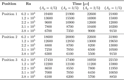
second recorded image, and it has to be adjusted with the mean velocity in the field. In fact, if this parameter is not correct the time between two different frames is either too short or too long to allow the correct displacement of each particle to be recorded. Consequently, it is impossible to evaluate the velocity field of the flow analyzed. Table2.3shows the time between pulses used in this work for each run; in particular, smaller time intervals were used for faster fields and larger ones in slower velocity fields. In a recent work [45], Corvaro et al. pointed out that while considering non-intrusive PIV technique, laser power and acquisition time affected the measurement by causing localized heating of the surfaces (upper and lower) to be stricken by the laser. To reduce this effect, in our study the chosen frequency was 6.1 Hz and in a relative time record of about 30 s, 200 couples of images were acquired. Moreover, no preview mode was used for ten minutes before the acquisition.
Table 2.3: Time between pulses values used for each experimental test. Rayleigh number is the ideal value calculated through equation2.2.
Position Ra Time [µs] (Ap= 4/5) (Ap= 3/5) (Ap = 2/5) (Ap= 1/5) Position 1 6.2 × 10⁴ 19400 21900 22600 21800 1.2 × 10⁵ 13600 15500 16900 15800 2.2 × 10⁵ 9600 10900 12600 12000 3.1 × 10⁵ 7800 8700 10400 10200 3.8 × 10⁵ 6700 7350 9000 9150 Position 2 6.2 × 10⁴ 18600 20000 22600 31900 1.2 × 10⁵ 12600 12850 13000 19650 2.2 × 10⁵ 8800 8700 8200 13000 3.1 × 10⁵ 7250 7050 6500 10500 3.8 × 10⁵ 6300 6100 5500 9150 Position 3 6.2 × 10⁴ 17450 17400 16950 22150 1.2 × 10⁵ 12200 12100 11200 15900 2.2 × 10⁵ 8650 8550 7800 11950 3.1 × 10⁵ 7000 7050 6450 10050 3.8 × 10⁵ 6100 6200 5700 8850
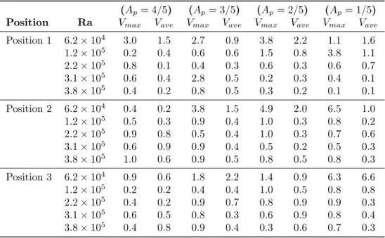
The repeatability of the experiment is a relevant indicator of the quality of mea-surements. For each case, the same test was repeated with the same initial boundary
conditions; additionally, 200 image couples were acquired every 10 min in 1 hour and a created database was used to evaluate the magnitude of the average and maximum velocity. Table2.4shows for each case the standard deviation σ of repeated measure-ments; standard deviation was calculated for the maximum and average value of the velocity field.
Table 2.4: Standard deviation of repeated measurements for each case study.
(Ap= 4/5) (Ap= 3/5) (Ap= 2/5) (Ap= 1/5)
Position Ra Vmax Vave Vmax Vave Vmax Vave Vmax Vave
Position 1 6.2 × 10⁴ 3.0 1.5 2.7 0.9 3.8 2.2 1.1 1.6 1.2 × 10⁵ 0.2 0.4 0.6 0.6 1.5 0.8 3.8 1.1 2.2 × 10⁵ 0.8 0.1 0.4 0.3 0.6 0.3 0.6 0.7 3.1 × 10⁵ 0.6 0.4 2.8 0.5 0.2 0.3 0.4 0.1 3.8 × 10⁵ 0.4 0.2 0.8 0.5 0.3 0.2 0.1 0.1 Position 2 6.2 × 10⁴ 0.4 0.2 3.8 1.5 4.9 2.0 6.5 1.0 1.2 × 10⁵ 0.5 0.3 0.9 0.4 1.0 0.3 0.8 0.2 2.2 × 10⁵ 0.9 0.8 0.5 0.4 1.0 0.3 0.7 0.6 3.1 × 10⁵ 0.6 0.9 0.9 0.4 0.5 0.2 0.5 0.3 3.8 × 10⁵ 1.0 0.6 0.9 0.5 0.8 0.5 0.8 0.3 Position 3 6.2 × 10⁴ 0.9 0.6 1.8 2.2 1.4 0.9 6.3 6.6 1.2 × 10⁵ 0.2 0.2 0.4 0.4 1.0 0.5 0.8 0.8 2.2 × 10⁵ 0.4 0.2 0.9 0.7 0.8 0.9 0.9 0.3 3.1 × 10⁵ 0.6 0.5 0.8 0.3 0.6 0.9 0.8 0.4 3.8 × 10⁵ 0.4 0.8 0.9 0.4 0.3 0.6 0.7 0.3
2.1.3
Data analysis
A wide number of acquired images was processed to obtain velocity maps. The size of the images was 1344x1024 pixels with an interrogation area of 32x32 pixels. Images were masked to analyze only the area within the cavity where the seeding is present. Signals were processed by using an adaptive cross-correlation function provided in the Dantec Dynamic software of the PIV system, and also a moving-average validation method was used to accept or reject vectors from the cross-correlation process. A 50% overlap of the areas was used both in the horizontal and vertical directions. The algorithms used for post-processing are described in order to their application. Enhanced information about the used algorithm can be found in Dantec Dynamics user’s guide [58].
• Image arithmetic: this method enables arithmetic on pixel values. Addition, subtraction, multiplication and division operations can be executed between two set of images. In our case, an image of the empty cavity was acquired before the entering of the seeding and subtracted to the 200 images performing the measurement. In this way, it is possible to eliminate the reflections on the edges of the cavity and on the surfaces of the obstacle. Figure2.5shows an example of the output file.
(a) Single image acquires through PIV run. (b) Image obtained applying the image arith-metic method.
Figure 2.5: Experimental images.
• Define mask and image masking: the size of the image is 1344x1024 pixel but the enclosure covers an area of about 800x800 pixel when the CCD camera is positioned at a distance of 0.5 m from the test cell. To elaborate only the interesting area within the cavity a mask was applied. The mask can be composed of three types of shapes (rectangles, polygons and ellipses) and the shape location and size can be specified. Figure 2.6 shows the five rectangular shapes that were used to cover the surfaces outside the enclosure and the baffle, only the area interested by the seeding is processed through following algorithms as in figure2.6.
(a) Mask definition. (b) Output image obtained appling the image masking method.
• Adaptive cross-correlation: the adaptive correlation method calculates ve-locity vectors with an initial interrogation area (IA) of the size N time the size of the final IA and uses the intermediary results as information for the next IA of smaller size until the final IA size is reached. In our study three refinement steps were performed; the starting interrogation area was 128x128 pixel until to an IA of 32x32 pixel. To compensate the loss of vector field resolution during the pro-cessing, an overlap of 50% IA was used both in horizontal and vertical directions. A moving-average validation method was used to accept or reject vectors from the cross-correlation process. Based on this validation method, individual vectors are compared to the local vectors in the neighborhood vector area. If a vector differs too much in intensity from its neighbors, it is removed and replaced by a vector, which is calculated by local interpolation of the vectors present in the surrounding. Velocity vectors are estimated from mean particle displacement inside interroga-tion areas (IA). Mathematically, D(−→X; t0, t+1) ≈∫
t+1
t0 u
[−→
X(t), t]· dt, where D is the displacement and u is the velocity, is the main formula used to calculate velocity vectors. This formula is transformed into an algebraic equation using a Central Difference Scheme. This scheme is equivalent to a three-point symmetric algorithm for the evaluation of d(−→X)/dt, with a reference ’point’ created at the time t+1 (See figure2.7).
Figure 2.7: Vector velocity map obtained through the application of the adaptive cross-correlation method; green vectors are external to the cavity domain and were not considered during the post-processing.
• Coherence filter: feature trackers and cross-correlation may occasionally yield completely wrong velocity vectors. To enhance the result of measurement, coherence-based post-processing is applied to the raw velocity field obtained. The coherence filter modifies a velocity vector if it is inconsistent with the dominant surrounding vectors. All vectors within the radius of 30 pixels are used for validation. Figure2.8 shows an output image.
Figure 2.8: Vector velocity map obtained through the application of the coherence filter method. Some green vectors are external to the cavity domain and they are not considered during the post-processing. However, a few number of green vectors is within the cavity and represent the result of the algorithm.
• Vector statistics: this method calculates statistics from multiple velocity vector maps. Only the valid vectors included in an interrogation area are used to calculate velocity map; bad vectors are discarded. Graphically speaking, results are presented as a vector map of mean velocity vectors as in figure2.9. A lot of other statistical quantities are calculated as well (position in pixel and mm, horizontal and vertical velocity components displacement, standard deviation and sum of variances, correlation coefficient, number of samples and vector length).
Figure 2.9: Vector velocity map obtained as result of the statistical analysis of 50 image couples.
The result of the post-processing is represented by two velocity maps: scalar map and streamlines (see figure 2.10). Through this two couple of images, a qualitative comparison of experimental and numerical results was possible.
(a) Velocity scalar map. (b) Streamlines.
Figure 2.10: Results of the experimental post-processing.
2.1.4
Two-dimensionality of the flow
Previous numerical studies [11,12] confirmed the supposition of two-dimensionality of the flow. In accordance with those authors, to ensure the absence of end effects, the experimental test was performed at the central plane of the enclosure. However, to experimentally verify the 2D behavior of the flow, the velocity fields were investigated at two other different square cross-sections. Figures 2.11, 2.12and 2.13 show the velocity profile of the horizontal and vertical components measured in three parallel vertical planes at 1/2 of the cavity height: the measurement central plane and two other planes at a distance of 5 cm to the front and to the back. The cases with an aperture ratio of Ap= 1/5and Ra of 3.8 × 10⁵were considered for all divider positions.
The x-position has been normalized by the cavity width (L = 0.05m). The value 0 corresponds to the position of the hot wall and the value 1 coincides with the cold one. The good concordance of the velocity profile can be seen for all cases and confirms the supposition of 2-dimensionality of the flow at the central plane. A small discordance of values is present near the hot wall and at the left side of the baffle when the obstacle is positioned in the middle of the cavity.
2.1.5
PIV measurements convergence
To ensure that stochastic phenomena did not affect the measure of the velocity field, a PIV measurement convergence was performed in two areas of the flow for three different cases. The aperture ratio of Ap = 1/5for all the positions of the baffle
was analyzed at Ra of 3.8 × 10⁵ (corresponding at ∆T = 40 °C). Figures 2.14, 2.15
show the variation of the average velocity in two specific positions when adding a further image for the calculation of the velocity field. In figure2.16 the maximum value of velocity within the cavity was plotted. The x-axis represents accumulated PIV
Figure 2.11: Average velocity profile at H/2 for Ap= 1/5, p = 3L/10 and Ra = 3.8 × 10⁵.
Figure 2.12: Average velocity profile at H/2 for Ap= 1/5, p = L/2 and Ra = 3.8 × 10⁵.
snapshot. The coordinates of the interesting areas have been normalized by the cavity height: x/L = 0 corresponds to the hot wall while the value 1 coincides with cold ones. y/L= 0locates the lower cavity wall and the value 1 the cavity top. The first position is located in the middle of the cross-section near the hot wall and the second one on the opposite side (next to the cold wall). Results seem to guarantee that 50 images were enough to reach the average velocity convergence during experimental analysis. For the first 20 images, stochastic errors produced very high variable results, especially for the maximum velocity and for the average value near the hot wall.
Figure 2.14: PIV realization convergence at H/2 and x/L = 0.1 for Ap= 1/5 and Ra =
3.8 × 10⁵
.
Figure 2.15: PIV realization convergence at H/2 and x/L = 0.9 for Ap= 1/5 and Ra =
3.8 × 10⁵.
2.2
Numerical technique
Natural convection in a square cavity with an inner vertical baffle was numerically studied through a Computational Fluid Dynamic (CFD) software. The governing
Figure 2.16: PIV realization convergence for Ra = 3.8 × 10⁵.
equations for a fluid include the conservation of mass, momentum and energy. These equations are presented in integral or differential (PDE) form to partial derivatives, whose resolution leads to the knowledge of all variables of the problem (velocity field, pressure range, etc.). However, they cannot be solved analytically in most engineering problems, except for a limited number of cases; CFD allows the resolution of such equations in all cases by admitting several approximations, and hence with a known error. By determining the numeric values of interesting variables in discrete spaces of space and time (grid of calculation, or mesh), CFD technique allows substituting partial integrals and derivatives with a set of discrete algebraic expressions, leading to a numerical and non-analytical resolution of the problem.
After the identification of the domain, the followed CFD procedure consists of three steps: • Pre-processing 1. Geometry 2. Mesh 3. Physics 4. Solver setting • Solve 1. Compute solution • Post-Processing 1. Examining results
The reproduction of the geometry of the physical problem, the definition of boundary types and the application of the grid to the interested areas were achieved with Gambit 2.3.16 software. The modeling of the physical problem, the definition of the boundary conditions and all simulations were performed using ANSYS Fluent 12.1.4. Finally, the isotherms with the relative Nusselt number were evaluated and stream functions and velocity maps obtained were compared to the experimental data to validate the numerical results and the adopted model.
The definition and discretization of the physical model (geometry representation and grid generation) is the first step of the process. Usually, for scientific purposes, simple, easily modellable but detailed geometries were used. Then, the problem is transferred from its continuous domain to a discrete representation of the geometry through the application of a mesh or a grid. In the continuous domain, each flow variable is defined at every point in the domain. For instance, the pressure p in the continuous 1D domain shown in the figure below would be given as
p= p(x) 0 < x < 1 (2.1)
In the discrete domain, each flow variable is defined only at the grid points. So, in the discrete domain shown in figure2.17, the pressure would be defined only at the N grid points: pi= p(xi); i = 1, 2, ..., N.
Figure 2.17: Visualization of the differences between continuous and discrete domain.
In a CFD solution, it can be directly solved for the relevant flow variables only at the grid points. The values at other locations are determined by interpolating the values at the grid points. The governing partial differential equations and boundary conditions are defined in terms of the continuous variables. These can be approximated in the discrete domain in terms of the discrete variables. The discrete system is a large set of coupled, algebraic equations in the discrete variables. Setting up the discrete system and solving it (which is a matrix inversion problem) involves a very large number of repetitive (iterative) calculations performed by computers. ANSYS Fluent uses the finite-volume method for discretization, based on the mesh cells. In the finite-volume approach, the integral form of the conservation equations is applied to the control volume defined by a cell to get the discrete equations for the cell. The code directly solves for values of the flow variables at the cell centers; values at other locations are obtained by suitable interpolation.
2.2.1
Geometry and mesh
The physical phenomenon of natural convection in a differentially heated cavity with a vertical baffle was experimentally studied in a parallelepipedal enclosure built with a certain number of external volumes. These volumes have to be considered in the modeling of the physical domain because they took part in the thermal interaction between air and active walls. Some simplifications can be performed:
• as described in Chapter 1, the inner flow was assumed to be 2-dimensional so the considered computational domain was a cross-section of the entire 3D
(a) Geometry model for numerical simulation. (b) Computational geometry used dur-ing numerical simulation.
Figure 2.18: Computational geometry.
Once the geometry is completed, a discretization of the computational domain has to be performed. The choice of the mesh has a significant impact on the accuracy and stability of the computation as well as the computational time it takes for the solution to converge. Referring to the work of Paroncini [59] and Acharya and Jetli [17] a quadrilateral structured mesh was built. A fine mesh was chosen to cover the internal area of the cavity, where the solution has to be the most accurate. A sparse mesh covered the external geometry where the solution is less important and imprecise results (within certain limits) were deemed acceptable. Wall boundary type was imposed for all the edges of the geometry. Figure 2.19shows the cavity with its mesh and relative material types. The influence of the mesh on the numerical results was observed. This study allowed to choose the number of cavity cells to achieve a
good compromise between the accuracy of the results and the computational times that are usually increasing as the number of cells increases.
Figure 2.19: Computational grid.
2.2.2
Pure convection model
Once the meshed geometry is completed using Gambit software, it is exported into a file type compatible with the solver so that it may be imported into ANSYS Fluent where the problem is modeled. In order to solve heat transfer problems, the user must activate the relative physical models and supply both the relevant thermal boundary conditions and material properties.
In pure natural convection, the strength of the buoyancy-driven flow is measured by Rayleigh number:
Ra= gβ∆T L
3
να (2.2)
where g is the modulus of the gravity vector, β is the thermal expansion coefficient, ∆T is the temperature difference between hot and cold walls, L is the characteristic length of the problem domain, ρ is the fluid density, ν represents the dynamic viscosity and α is the thermal diffusivity. All these properties of air have been considered as a function of temperature at atmospheric pressure except for the density. For density description, ANSYS Fluent allows the user to apply the Boussinesq model to heat transfer problems. It ensures a faster convergence if the problem is formulated with fluid density as a function of temperature. This model treats density as a constant value in all solved equations, except for the buoyancy term in the momentum equation:
(ρ − ρ0)g ≈ −ρ0β(T − T0)g (2.3)
where ρ0 is the (constant) density of the flow and T0 is the operating temperature.
The equation above is obtained by applying the Boussinesq approximation ρ = ρ0(1 −
β∆T ) to eliminate ρ from the buoyancy term. This approximation is valid when β(T − T0) ≪ 1(changes in density are small). The Boussinesq approximation can be
used for the description of this problem because the temperature difference is little (as a consequence also the density variation is limited) and Rayleigh numbers are appreciably low than 108. This last condition about Ra indicates a buoyancy-induced laminar flow,
In the solid, only conduction heat exchange has been considered; the Plexiglas®characteristics
(see table 2.1) have been introduced into the software library through an external input file. The temperature of the entire right and left walls were set respectively at T = Tc and T = Th. Since the dimension of the two Plexiglas®volumes can
guaran-tee an adequate thermal insulation, the heat exchange was enabled on the external Plexiglas®walls. At the solid/fluid interface between the inner part of the cavity (air)
and the solid volumes (upper and lower walls and baffle edges), Fluent automatically generates a "shadow" zone so that each side of the wall is a distinct wall zone with a distinct material. Here, a coupled boundary condition was set and no additional thermal boundary conditions are required because the solver will calculate heat transfer directly from the solution in the adjacent cells. Summarizing, the thermal boundary conditions can be written as:
u ( 0,3L 5 ≤ y ≤ 8L 5 ) = u ( L,3L 5 ≤ y ≤ 8L 5 ) = u ( 0 ≤ x ≤ p −d 2, 3L 5 ) = = u ( p −d 2, 3L 5 ≤ y ≤ 3L 5 + h ) = u ( p − d 2 ≤ x ≤ p + d 2, 3L 5 + h ) = = u ( p+d 2, 3L 5 ≤ y ≤ 3L 5 + h ) = u ( p+d 2 ≤ x ≤ L, 3L 5 ) = u ( x,8L 5 ) = 0 (2.8) ∇T (x, 0) = ∇T ( x,11L 5 ) = 0 (2.9) T(0, y) = Th (2.10) T(L, y) = Tc (2.11)
where the system reference and coordinates are in accordance with the figure2.18. Numerical results were obtained through pressure based segregate solvers. It was originally designed for incompressible and mildly compressible flow. The pressure-based solver uses a solution algorithm where the governing equations are solved sequentially. Because the governing equations are non-linear and coupled, the solution loop must be carried out iteratively in order to obtain a converged numerical solution. In the segregated algorithm, continuity, momentum and energy equations are solved sequentially segregated from one another and linearized implicitly with respect to the
equation’s dependent variable. The segregated algorithm is memory-efficient since the discretized equations need only to be stored in the memory one at a time. However, the solution convergence is relatively slow, as much as the equations are solved in a decoupled manner. Using this solution method, the velocity field is obtained from the momentum equation and the pressure field is determined by solving a pressure equation which is itself obtained by manipulating the continuity and momentum equations in such a way that the velocity field, corrected by the pressure value satisfies continuity. The semi-implicit SIMPLE algorithm was employed for the pressure-velocity coupling. This scheme uses a relation between velocity and pressure corrections to enforce mass conservation and to obtain the pressure field. Three steps are necessary:
1. an approximation of the velocity field is obtained by solving the momentum equation. The pressure gradient term is calculated using the pressure distribution from the previous iteration or an initial guess;
2. the pressure equation is formulated and solved in order to obtain the new pressure distribution;
3. velocities are corrected and a new set of conservative fluxes is calculated. The spatial discretization scheme applied is the Green-Gauss Cell-Based gradient. These gradients are needed to determine the scalar values at the cell faces, the secondary diffusion terms and the velocity derivatives. In this case, the Green-Gauss theorem is applied to each cell and the face value of the scalar is taken as the arithmetic average of the values of the neighboring cells.
The Body Force Weighted scheme is applied for pressure discretization. This scheme computes the face pressure by assuming that the normal gradient of the difference between pressure and body forces is constant. This works well with problems that involve buoyancy in which the body forces are known a priori in the momentum equations.
With regards to spatial discretization, a second-order upwind scheme is adopted for both the momentum and energy equations. By default, Fluent stores discrete values of the scalar at the cell centers. However, face values are required for the convection terms and must be interpolated from the cell center values. This is accomplished using an upwind scheme. The face value of the scalar is derived from quantities in the cell upstream, or "upwind", relative to the direction of the normal velocity. The Second Order scheme is chosen as the flow does not go always in one direction and this scheme offers a more accurate solution in such cases.
Under-relaxation factors are employed in numerical computing to stabilize numerical schemes involving iterative procedures. They are used to improve convergence of such numeric schemes, however, they come at the penalty of increasing time taken to the solution of the desired accuracy. The under-relaxation factors have no effect on the solution, though they will influence the number of iterations (and hence time) used to converge to the desired level of accuracy.
At the end of each solver iteration, the residual sum for each of the conserved variables is computed and stored. On a computer with infinite precision, these residuals will go to zero as the solution converges. On an actual computer, the solution has converged when all the residuals’ values are lower than the residual monitor value. For single-precision computations (the default for workstations and most computers), residuals can drop as many as six orders of magnitude before hitting round-off. Double-precision residuals, used in the described simulations, can drop up to twelve orders of
u
∂x + v∂y = α ∂x2 + ∂y2 −
1 ρcp
∇ · qr (2.12)
The local divergence of the radiative flux (∇ · qr) in the energy equation is related
to the local intensities by:
∇ · qr= κ ( 4πIb(r) − ∫ 4π I(r, Ω)dΩ ) (2.13) To obtain the radiation intensity field and ∇·qrit is necessary to solve the Radiative
Transfer Equation (RTE). This equation for an absorbing, emitting, and scattering medium at position r in the direction s is:
dI(r, s) ds + (a + σs)I(r, s) = an 2σT 4 π + σs 4π ∫ 4π I(r · s′)Φ(s, s′)dΩ′ (2.14) It is important to note that the RTE has to be solved in a 3D domain whereas the flow field is solved in 2-dimensional coordinates.
Of the five different radiation models available in ANSYS Fluent [60] the Discrete Ordinates (DO) model is the only that can deal with radiation problems with both semi-transparent walls and participating and non-participating media. Moreover, the DO radiation model can also be used to solve radiative heat transfer problems involving both grey and non-grey surfaces. Computational cost is moderate for typical angular discretizations and memory requirements are modest.
DO radiation model solves a finite number of radiative transport equations given by the amount of discrete defined solid angles. These solid angles, based on a control angles discretization, are used to discretize each octant of the angular space at any spatial location. In the two-dimensional calculation, four octants are discretized in Nθ× Nϕ solid angles based on the polar (θ) and azimuthal (ϕ) angles respectively,
making a total of 4NθNϕ directions altogether. These angles are measured with respect
to the global Cartesian system (x, y, z).
Although this model can take into consideration the participating medium, air is considered as transparent in the present study. The Plexiglas®upper walls are assumed
semi-transparent while all other surfaces have the following properties: grey diffuse. The emissivity of various walls is shown in table 2.5. The initial condition are the same of the pure natural convection case, u = v = 0, p = 0 and T = Tave. For the
velocity field within the cavity, the no-slip boundary condition is assumed. For the energy equation, the left wall is at Th, the right wall is at Tc and the upper and lower