LAMINAR FORCED CONVECTION IN A CYLINDRICAL
COLLINEAR OHMIC STERILIZER
by
Tommaso PESSO and Stefano PIVA*
Department of Engineering (ENDIF), University of Ferrara, Ferrara, Italia
Original scientific paper1
https://doi.org/10.2298/TSCI151105124P
The present work deals with a thermo-fluid analysis of a collinear cylindrical ohmic heater in laminar flow. The geometry of interest is a circular electrically insulated glass pipe with two electrodes at the pipe ends. For this application, since the electrical conductivity of a liquid food depends strongly on the temperature, the thermal analysis of an ohmic heater requires the simultaneous solution of the electric and thermal fields. In the present work the analysis involves decoupling the previous fields by means of an iterative procedure. The thermal field has been calculated using an analytical solution, which leads to fast calculations for the temperature distribution in the heater. Some considerations of practical interest for the design are also given.
Key words: ohmic heating, forced convection, laminar flow Introduction
Sterilization of liquid foods by continuous ohmic heating is of growing interest in the industry. This process is based on the internal heat generation in a material subjected to an electric field and offers significant advantages over conventional food processing methods, both in terms of quality and quickness of the process [1]. Recent reviews of this technology are given by Varghese et al. [2] and Sakr and Liu [3] both for developments and applications.
The ohmic heating of a liquid food takes place in an apparatus where the food is the conductive medium and the electrodes are in intimate contact with the product [4]. These elec-trodes are generally separated by a tube which is electrically insulating. There are two main generic industrial configurations for continuous operation [4]:
– transverse configuration: the product flows parallel to the electrodes and perpendicularly to the electric field. In this case the electrodes are generally plane or coaxial, and
– collinear configuration: the product flows from one electrode to the other one and the flow is parallel to the electric field.
Reliable mathematical modelling of these configurations can provide important infor-mation for the calculation of sterility or cooking levels.
In general, since the electrical conductivity of liquid foods depends strongly on the temperature, the thermal analysis of an ohmic heater requires the coupled solution of the electric and thermal fields [5]. An in-depth review of these topics is given by Goullieux and Pain [4]. However, as evident in this review [4], not many studies have been undertaken to examine the thermo-fluid features of collinear ohmic heaters for the treatment of homogeneous fluids.
––––––––––––––––––
The present work deals with the thermo-fluid analysis of a collinear cylindrical ohmic heater in laminar flow for the treatment of apricot puree and similar fluids. The electrical prop-erties of this food are available from the literature [6]. All the other fluid propprop-erties, except for the electrical conductivity, are considered to be constant. The fluid is assumed to be homoge-neous. Since it is commonly supposed that the presence of small solid particles in the fluid has negligible effects on the flow [7], the assumption of homogeneous fluid is also valid for liquids containing small solid particles, such as fruit. Their presence becomes significant for high solid volume fractions and when the characteristic dimension of the particles is the same as that of the pipe [7]. Under the quoted assumptions it is possible to obtain an analytical solution for the thermal field [8], which leads to fast calculations for the temperature distribution in the heater. The analysis decouples the electric and thermal fields and uses an iterative procedure. In the initial step, the electric field is calculated, for a known temperature distribution, by means of a numerical method. In the following step, the thermal field is calculated by means of an analyt-ical solution. This is to laminar forced convection of a homogeneous fluid in a circular pipe with temperature dependent internal heat generation and convective boundary conditions [9].
Mathematical model
System description
The geometry of interest is schematically shown in fig. 1. A fluid flowing in a circular electrically insulating glass pipe is heated through two electrodes placed at the pipe ends.
The length of the heating section is 2.5 m and the inner and outer diameter of the pipe 50 mm and 60 mm, respectively. At the external surface of the pipe the thermal cou-pling with the ambient is considered. The ambient temperature is taken as Ta = 20 °C.
The inlet temperature of the fluid is To = 40 °C.
The working fluid is apricot puree. The dif-ference of direct potential imposed at the electrodes is V = 2304 V. This value has been chosen by means of the procedure dis-cussed in Appendix A.
Basic assumptions
In order to analyse a very complex problem such as a collinear ohmic heater, a number of simplifying assumptions are necessary.
The fruit puree is considered to be a homogeneous fluid. All the thermophysical prop-erties of the fluid, except for the electrical conductivity, are assumed to be constant.
Since the fruit is mainly composed of water, its thermophysical properties are consid-ered to be the same as those for water. The electrical conductivity of the fluid is expressed as a linear function of the temperature:
o 1 o T To
(1)
where o and o for apricot puree are given by [6]:
o 0.998 S m Heating section 2.5 m Circular stainless steel electrode Circular stainless steel electrode Fluid inlet 40 °C Fluid outlet 105 °C Glass tube
o 0.015 1 K
Over any cross-section of the pipe, the current density is assumed to be constant. When solving the thermal field, the internal heat generation is expressed as a linear (decreasing) function of the temperature. Viscous dissipation in the fluid and axial heat conduction in the wall of the pipe and in the fluid are neglected.
Governing equations and solution strategy
For a pipe with electrically insulated walls, where the current density is constant over any given cross-section of the pipe, the electric potential, U, is the solution of the following differential equation [6]: 0 xU x (2)
with the boundary conditions:
0 2 x V U (3) 2 x L V U (4)
The thermal field, for a homogenous fluid in laminar flow in a circular pipe at high Peclet number (Pe > 50), is the solution of the following differential equation:
2 f 1 gen 2 1 2 r T T W k r q D x r r r (5)
with the boundary conditions:
for x = 0 T
0,r To (6) for 0 < x < L 0 0 r T r (7) for 0 < x < L
2 a
2 r D r D T k K T T r (8)The local internal heat generation is given by:
gen U q x T x 2 (9) It is easy to demonstrate that, for fluids characterized by a thermal conductivity in-creasing with temperature, the ohmic internal heat generation decreases with the temperature (see Appendix B for the demonstration).Equations (2) and (5) are coupled through eqs. (1) and (9). Then, in order to solve the system of equations given by eqs. (2)-(9), an iterative procedure is adopted.
This iterative procedure is detailed as follows. An axial distribution of the bulk temperature is assumed.
For a known axial distribution of the bulk temperature, the electrical conductivity is calcu-lated by eq. (1). Then, the conservation equation for the electric field, eq. (2), with boundary conditions eqs. (3) and (4), is solved by means of a numerical procedure.
The internal heat generation distribution is calculated by eq. (9) and is linearized as a func-tion of the known axial distribufunc-tion of the bulk temperature.
The energy conservation eq. (5) is treated analytically by means of the solution proposed in [8]. A new axial distribution of the bulk temperature is calculated and the procedure is repeated from second step.
Thermal field
While the numerical solution of eq. (2) with the boundary conditions of eqs. (3) and (4), is straightforward, some details about the solution of the thermal field are necessary.
When expressing the internal heat generation as a linear function of the temperature, eq. (5) becomes:
2 f 1 o o o 2 1 1 2 r T T W k r q T T D x r r r (10)Equation (10) is completed by the boundary conditions, eqs. (6)-(8). The solution of the eqs. (6)-(8) and (10) is given by [8]:
a * o 0 1 o i i i 2 2 a o 1 1 0 1 1 1 1 1 , exp 2 w i T x r T S J S r S A x f T T S J S R S J S S
(11) where f i w k R KD (12)
2 o o a o i o f a o 1 4 q T T D S k T T (13) 2 2 o o i 1 f 4 q D S k (14) * i Pe 2 x x D (15) i 2 r D (16)
1 1 2 o 1 0 1 2 2 o i i 2 0 1 1 1 1 1 0 0 i 1 1 2 2 2 2 i i 0 0 1 1 d 1 d 2 1 d 1 d w S S J S S f f ξ J S R S J S S A f f
(17)
i 2 2 i pe , i exp 2 1 1 i,1, i f F (18) i i (19) 2 i 1 i i 1 1 2 2 2 S (20)The parameters i are the roots of the following transcendental equation:
i i 1 1 d 1 0 d r 2 w r f f r R (21)
and they can be easily calculated by means of a numerical procedure.
The bulk temperature distribution, used in the present iterative procedure as the axial distribution of the temperature, is given by:
1 2 b a * i 1 i i i a o 1 i 1 i 0 2 1 o o 2 2 2 0 1 1 1 1 1 1 1 d 1 4 exp d d 8 1 2 i w T x T f S A x f T T J S S S J S R S J S S S S
(22)Results and discussion
In the present context, the influence of the mass flow rate of puree and of the thickness of the thermal insulation on both the heat transfer quantities and the radial and axial temperature distribution are analysed.
The external convective heat transfer coefficient is estimated as 5 W/m2K for natural
convection on a horizontal pipe. The external radiative heat transfer has been taken as 5 W/m2K.
The pipe is considered as being surrounded by a layer of insulating material and the effect of different thicknesses of the insulation is discussed below.
For the calculation of the thermal field, eq. (11), twenty eigenvalues, i , were taken,
thereby ensuring accurate calculations [8].
Although the heat generating distribution is 2-D, eq. (10), the effect of the dependency of the electrical conductivity of the fluid on the temperature, eq. (1), is discussed in terms of the bulk temperature. In fig. 2 a bulk temperature distribution typical for the present analysis, is shown. For the present application, inlet and outlet temperatures of 40 °C and 100 °C,
respectively, form the most frequent case. This bulk temperature distribution is not linear, with an evident trend to lower values for long distance from inlet.
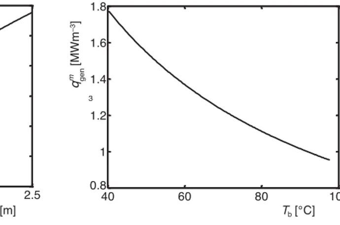
In fig. 3 a calculated heat generating distribution typical for the present analysis, is represented as a function of the bulk temperature. Due to the non-linear trend of the bulk tem-perature shown in fig. 2, also the heat generating distribution is not linear.
0 0.5 1 1.5 2 2.5 40 50 60 70 80 90 100 x [m] 40 60 80 100 0.8 1 1.2 1.4 1.6 1.8 Tb[°C] 3 ge n m q [MWm –3] Tb [ oC]
Figure 2. Typical distribution of the bulk
temperature Figure 3. Typical distribution of the heat generating term as a function of the bulk temperature
The internal heat generation decreases as the bulk temperature increases. This decrease is nearly linear. The internal heat generation is very high in the inlet section (of the order of 2 MW/m3)
while near the outer section, the internal heat generation is lower (of the order of 1 MW/m3).
The influence of the thermal insulation covering the glass pipe on the outlet tempera-ture is analysed for the cases summarised in tab. 1. The main results are summarized in tab. 2. As expected, the outlet bulk temperature increases with the thickness of the thermal insulation. It can be observed that an insulation given by 5 cm of fibreglass is a reasonable choice for the present application, because the reduction of heat dissipation is about 28.5% of the maximum reduction (adiabatic condition) that we can calculate with the results given in tab. 2.
Table 1. Influence of the thermal insulation: Table 2. Main results: influence of cases of analysis the thermal insulation
Case Mass flow Insulation Rw Case Rw So Sl2 Tout
1 82.5 kg/h no 1.1 1 1.1 –96.6 –13.4 98 °C
2 82.5 kg/h 5 cm fibreglass 4.3 2 4.3 –98.2 –13.4 100 °C
3 82.5 kg/h 17 cm fibreglass 10 3 10 –98.6 –13.4 101 °C
4 82.5 kg/h infinite layer →∞ 4 →∞ –102.1 –13.3 105 °C
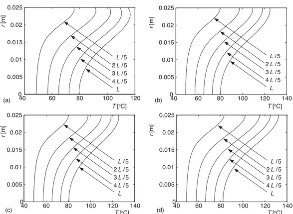
The radial temperature profiles for these cases of tab. 1 are shown in fig. 4. It can be observed that the profiles corresponding to the same axial stations are quite similar in shape also for different degrees of thermal insulation. The radial temperature profiles are character-ized by a maximum at r ≈ 0.8R, which denotes that the heat is radially transferred both to the environment and to the fluid flowing in the core of the duct. Moreover, each radial temperature profile is far from being uniform. This could be an important consideration for designers of food equipment, as it means that the thermal treatment of the food is non-uniform.
40 60 80 100 120 0 0.005 0.01 0.015 0.02 0.025 2L /5 4L /5 L L /5 3L /5 (a) (b) (c) (d) 40 60 80 100 120 140 0 0.005 0.01 0.015 0.02 0.025 2L /5 4L /5 L L /5 3L /5 40 60 80 100 120 140 0 0.005 0.01 0.015 0.02 0.025 2L /5 4L /5 L L /5 3L /5 40 60 80 100 120 140 0 0.005 0.01 0.015 0.02 0.025 2L /5 4L /5 L L /5 3L /5 r [m] r [m] r [m] r [m] T [oC] T [oC] T [oC] T [oC]
Figure 4. Radial temperature profiles at selected axial stations for the cases of study of tab. 3; (a) case N. 1, (b) case N. 2, (c) case N. 3, (d) case N. 4
The influence of the mass flow rate of the food on the outlet temperature is analysed for the cases summarized in tab. 3, characterized by the absence of thermal insulation. The main results are summarized in tab. 4. The design mass flow rate (Case 2 – see Appendix A for further details) is equal to 82.5 kg/h. Two further cases are examined: Case 1 is characterized by the reduction of the design mass flow rate of a 15% (mass flow rate equal to 61.9 kg/h) and Case 3 is characterized by an increment of the design mass flow rate of 50% (mass flow rate equal to 123.8 kg/h). Since the present problem is not linear, the relation between the mass flow and the outer temperature is far from being linear.
Table 3. Influence of the mass flow: Table 4. Main results: influence of cases of analysis (no thermal insulation) the mass flow
Case Mass flow Pe Rw Case Pe So Sl2 Tout
1 61.9 kg/h 2799 1.1 1 2799 –124.4 –13.8 133 °C
2 82.5 kg/h 3732 1.1 2 3732 –96.6 –13.4 98 °C
3 123.8 kg/h 5598 1.1 3 5598 –78.9 –13.0 74 °C
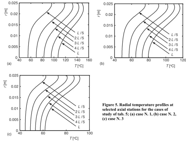
The radial temperature profiles for the cases of study of tab. 4 are depicted in fig. 5. As expected the temperature increases for decreasing values of the mass flow rate. Furthermore,
significant differences between the three different situations are not appreciable. As already
observed in the discussion of fig. 4, each radial temperature profile is characterized by the
environment and to the fluid flowing in the core of the duct. Furthermore, the radial distri-bution of temperature is not affected in its shape by either increasing or decreasing the mass flow rate. 40 60 80 100 120 140 160 0 0.005 0.01 0.015 0.02 0.025 2L /5 4L /5 L L /5 3L /5 (a) (b) (c) 40 60 80 100 120 0 0.005 0.01 0.015 0.02 0.025 2L /5 4L /5 L L /5 3L /5 40 60 80 100 0 0.005 0.01 0.015 0.02 0.025 2L /5 4L /5 L L /5 3L /5 r [m] r [m] r [m] T [oC] T [oC] T [oC] Concluding remarks
The method proposed for the analysis of a cylindrical collinear ohmic heater in lami-nar flow shows some features of interest.
The variation of the electrical conductivity of the food has a great influence on the predictions. For the calculation of the thermal field, the assumption of a linear dependency of the heat
generating term on the axial temperature distribution seems to be valid.
The method is fast and accurate. By means of this method, various considerations of prac-tical interest can be possible, such as the determination of the temperature of the fluid at the outer section of the heater, and the calculation of the heat lost to the environment. More-over, the possibility of calculating the radial temperature profiles at each cross-section of the duct is also of considerable relevance, since it can verify whether the thermal treatment of the food is uniform or not.
On the basis of the present results, some further considerations of practical interest on the design of cylindrical ohmic heaters are also possible.
Negative values of Sl2 introduce a stabilizing effect on the thermal field, since the internal
heat generation decreases as the temperature increases.
For the present ohmic heater, a value of Rw of at least 5 °C/W seems to be a reasonable choice.
Figure 5. Radial temperature profiles at selected axial stations for the cases of study of tab. 5; (a) case N. 1, (b) case N. 2, (c) case N. 3
Nomenclature
A – dimensionless constant
cp – specific heat of the fluid at constant pressure, [Jkg–1K–1]
Di – inner diameter of the pipe, [m] De – outer diameter of the pipe, [m] k – thermal conductivity, [Wm–1K–1] K – environment heat transfer
coefficient, [Wm–2 °C] Pe – Peclet number, (=WD/
qgen''' – internal heat generation, eq. (9), [Wm–3]
qo''' – internal heat generation at the reference temperature T'o, eq. (10), [Wm–3] Rw – thermal resistance, [KW–1] r – radial co-ordinate, [m]
So – dimensionless heat generating parameter S l
2 – dimensionless heat generating parameter
T – temperature, [°C]
Ta – environment temperature, [°C]
U – electrical potential, [V]
V – voltage, [V]
W – average axial velocity, [ms–1]
x – axial co-ordinate, [m] Greek symbols
– difference
– thermal diffusivity, [m2s–1]
o – coefficient of variation of the heat generating term with the temperature, [K–1], eq. (10)
– coefficient of variation of the electrical conductivity with the temperature, [K–1], eq. (1)
– root of eq. (21)
– auxiliary position, (√λ
– electrical conductivity, eq. (1), [Sm–1] Subscripts b – bulk f – fluid in – insulation o – inlet w – glass wall References
[1] Quarini, G. L., Thermal Hydraulic Aspects of the Ohmic Heating Process, J. Food Eng., 24 (1995), 4, pp. 561-574
[2] Varghese, K. S., et al., Technology, Applications and Modelling of Ohmic Heating: A Review, J. Food
Sci. Tech. Mys., 51 (2014), 10, pp. 2304-2317
[3] Sakr, M., Liu, S., A Comprehensive Review on Applications of Ohmic Heating (OH), Renewable
Sustainable Energy Rev, 39 (2014), Nov., pp. 262-269
[4] Goullieux, A., Pain, J. P., Ohmic Heating, in: Emerging Technologies for Food Processing (Ed. Da Wen Sun), Chap. 18, Elsevier Academic Press, London, 2005
[5] De Alwin, A. A. P., Fryer, P. J., Operability of the Ohmic Heating Process: Electrical Conductivity Effects,
J. Food Eng., 15 (1992), 1, pp. 21-48
[6] Icier, F., Ilicali, C., Temperature Dependent Electrical Conductivities of Fruit Purees During Ohmic Heating, Food Res. Int., 38 (2005),10, pp. 1135-1142
[7] Benabderrahmane, Y., Pain, J. P., Thermal Behaviour of a Solid/Liquid Mixture in an Ohmic Heating Sterilizer-Slip Phase Model, Chem. Eng. Sci., 55 (2000), 8, pp. 1371-1384
[8] Pesso, T. Piva, S., An Analytical Solution for the Laminar Forced Convection in a Pipe with Temperature Dependent Heat Generation, J. Appl. Fluid Mech., 8 (2015), 4, pp. 641-650
[9] Lienhard IV, J. H., Lienhard V, J. H, A Heat Transfer Textbook, 3rd ed., Available in the Web
Appendix A
Assuming that the wall of the pipe is adiabatic and that the internal heat generation and all the properties of the fluid are constant at the reference temperature Tm = (Tout –Tin) / 2,
from a global energy balance it follows:
out in
gen 2 i 4 p mc T T q L D (A.1)Under these assumptions, the electrical potential in the fluid is constant with value equal to U = V/L. Then, eq. (9) can be simplified:
2 gen m V q T L (A.2)Assuming an outlet temperature Tout = 105 °C, an inlet temperature Tin = 40 °C and a
mass flow rate ṁ = 82.5 kg/h, from eqs. (A.1), (A.2), and (1), it follows that V has to be of the order of 2000 V.
Appendix B
The local internal heat generation is given by:
2 gen U q x x (9)Remembering eq. (2), we can write:
U k
x
(B.1)
Then the local internal heat generation is:
2gen k
q x
(B.2)
decreasing with the temperature if the thermal conductivity of the fluid increases with the tem-perature.
Paper submitted: November 5, 2015 © 2017 Society of Thermal Engineers of Serbia. Paper revised: May 14, 2016 Published by the Vinča Institute of Nuclear Sciences, Belgrade, Serbia. Paper accepted: May 24, 2016 This is an open access article distributed under the CC BY-NC-ND 4.0 terms and conditions.