Properties and correlation of flares and coronal mass ejections and their possible relevance on the southern night sky background: a statistical study

(1)

UNIVERSITÀ DEGLI STUDI DI CATANIA

DIPARTIMENTO DI FISICA E ASTRONOMIA

DOTTORATO DI RICERCA IN FISICA XXX CICLO

ALESSIO COMPAGNINO

P

ROPERTIES AND CORRELATION OF

FLARES AND CORONAL MASS EJECTIONS

AND THEIR POSSIBLE RELEVANCE ON THE

SOUTHERN NIGHT SKY BACKGROUND

:

A

STATISTICAL STUDY

—-TESI DI DOTTORATO

—-Coordinator: Prof. V. Bellini

Tutor: Chiar.ma Prof.ssa F. Zuccarello Cotutors: Dott. P. Romano

Prof.ssa R. Caruso

(2)

i

The Sun, our star, can be considered a huge laboratory where we can study the interaction of a ionized gas with magnetic fields. In particular, the solar atmosphere (the outer layers of the Sun, those which are accessible to observations) is character-ized by phenomena that due their existence to localcharacter-ized magnetic fields: sunspots, faculae, filaments, active regions, bright points, coronal holes, etc. The occurrence of these phenomena is variable, depending on the so-called activity cycle, character-ized by a period of 11 years.

Moreover, in some situations, the magnetic field that permeates the active re-gions, from an initial potential field configuration (characterized by the minimum energy content), can slowly store energy, changing its configuration to more com-plex and more energetic ones. When the magnetic field configuration is not able to maintain its equilibrium, the stored magnetic energy is abruptly released, giving rise to phenomena that are generally termed as solar eruptions but that, depend-ing on their characteristics, are distdepend-inguished between flares, filament eruptions and coronal mass ejections.

In the last decades, the possibilities offered by new computer capabilities, new instruments and by satellite observations, have allowed us to understand many of the characteristics of these eruptions, as well as their effects on the Earth magneto-sphere and ionomagneto-sphere.

However, despite the progress in our comprehension of these phenomena, there are still many aspects that need to be clarified: how and where is the energy stored, what causes the trigger of the eruption, how the different phenomena are related to each other and how they can affect our environment, to cite only a few.

In this scenario, the work carried out in this Thesis has been motivated by three main questions:

• Are there preferential locations on the Sun where the magnetic field is prone to produce eruptive events ?

• What kind of correlation exists between flares (mainly confined to the solar atmosphere) and coronal mass ejections that, by definition, expel magnetized clouds into the interplanetary space ?

• Can the charged particles emitted during these events and arriving to the Earth ionosphere have a role in the observed variations of the night-sky background ?

The attempt to provide answers to the previous questions has been faced in this Thesis from an observational / statistical point of view.

(5)

More precisely, the dataset that have been used in order to answer the first two questions have been retrieved from public archives of flares and coronal mass ejec-tions relevant to the last two solar cycles (23 and 24), while in order to provide an answer to the third question, also data acquired by the Pierre Auger Observatory have been used.

The main results obtained in this Thesis can be summarized as follows:

• The spatial and temporal distribution of the flares analyzed show persistent domains of occurrence within well defined belts of longitude, with a behavior similar to the one observed for other activity phenomena, like the sunspots. • There is a temporal correlation between flares and CMEs for the 60 % of the

events analyzed; the time interval (between 10-130 minutes) however depends on the dataset used. Moreover, the majority of CMEs with highest velocities show a clear temporal correlation with flares.

• The variations in the night-sky background analyzed for the nights when a major impact of charged particles associated to CMEs was expected, could not be clearly correlated to these events.

The Thesis is organized as follows: in Chapter1we provide a brief introduction on the characteristics of the solar atmosphere and on the main eruptive phenomena occurring in the Sun. Chapters2 reports the main observational characteristics of flares and a description of the flare standard model, while Chapter3 describes the work carried out in order to study the occurrence of flares in preferential regions called Active Longitudes. The main observational characteristics of CMEs are re-ported in Chapter4. Chapters5 and6 report respectively on the statistical study of CMEs, on properties and correlation with flares. The study carried out using the data provided by the Pierre Auger Observatory in order to investigate the possible correlation between flares, coronal mass ejections and the variations in the night-sky background is reported in Chapter7. The discussion of the results obtained in this Thesis and the conclusions are reported in Chapter8.

(6)

v

(7)

1

Chapter 1

Introduction

1.1 Eruptive phenomena on the Sun

This chapter introduces the main characteristics of solar eruptive phenomena occur-ring in the solar atmosphere: filament eruptions, flares and coronal mass ejections (CMEs). These phenomena involve the interaction between localized magnetic fields and the hot ionized gas of the solar atmosphere (known as plasma i.e., a fluid that can be locally charged but globally electrically neutral, formed by both neutral and charged particles, such as electrons, protons and ions).

The Sun’s atmosphere is composed by three main regions which present dif-ferent temperature and density distributions (Figure1.1). The innermost layer, the photosphere, extends for about 500 km and is characterized by a temperature ranging between 5780 and 4300 K and a density of 2 × 10−4 kg m−3. Most of the sunlight

we observe is emitted from this layer. Above the photosphere there is the chromo-sphere, extending for ∼ 2500 km, with a temperature ranging from 4300 to ∼ 25000 K. A thin layer, called transition region, is located above the chromosphere: here the temperature suddenly increases from 104 _{to 10}5_{K. The outermost and hottest layer}

of the Sun is the corona, characterized by a temperature of about 2×106

K, and a density of ∼ 10−12_{− 10}−14kg m−3. A flow of plasma, such as electrons, ions, and

α particles, extending from the corona and propagating toward the interplanetary medium, is known as solar wind (Golub et al.,2009). Depending on the velocity, den-sity and source of origin of the solar wind, we can distinguish between two different regimes: the fast solar wind, with velocities of ∼ 500 - 800 km s−1at 1 AU and

orig-inating mainly in the polar regions (where dark features, with low emission in the Extreme Ultra Violet (EUV) and X-ray range, known as coronal holes, are located), and the slow solar wind, characterized by velocities of ∼ 300 - 400 km s−1at 1 AU,

originating mainly from equatorial regions.

In the solar atmosphere several features can be observed: sunspots, faculae, fila-ments, bright points, coronal loops, active regions. Their appearance and evolution is related to localized magnetic fields that emerge from the subphotospheric layers and later diffuse in the solar atmosphere. The number of sunspots present on the solar disc is quantified through the Wolf Number W = k(f+10g), where k is a pa-rameter that depends on the observational conditions (i.e., site, telescope, observer), while f and g indicate the total number of sunspots and sunspot groups, respectively, present on a certain day on the solar disk. The Wolf Number is not constant in time,

(8)

Chapter 1. Introduction 2

but follows a well defined periodicity (11-year), such that phases of maximum activ-ity are followed by phases of low activactiv-ity. Each 11-year period is called solar cycle.

At the beginning of each solar cycle the sunspots appear at latitudes of ∼ 40 de-grees, while in the following years the latitudes of appearance of sunspots slowly decrease and at the end of the cycle these features are observed close to the solar equator, following a pattern that is generally recognized by means of the Butterfly diagram. Moreover, within each solar cycle, the polarity of the sunspots is governed by the Hale’s Law, according to which in each solar hemisphere the preceding (i.e., the western) sunspot in each group has always the same polarity and in the other hemisphere the preceding sunspot has the opposite polarity. In the following cycle the situation is reversed (Zirin,1988).

Another characteristic of the solar magnetic activity is related to the presence of the so-called active longitudes, that are belts of longitude of about 15 degrees, char-acterized by the continuous emergence of magnetic flux and that therefore show a higher level of activity than the surrounding longitudes.

As we are mainly interested in solar phenomena that can give rise to eruptive events, we will describe in the following the main characteristic of these features / events, while we defer the reader toZirin(1988) for a complete description of other solar activity phenomena.

In the chromosphere and corona, in the Hα (6563 Å) and He II (304Å) lines respectively, we often observe dark elongated features, called filaments, which are characterized by a main axis, called spine (Figure 1.2), that presents features pro-truding laterally named barbs (indicated by white arrows in Figure1.2). Solar fila-ments appear dark due to the absorption that causes a lower emission with respect to the background atmosphere. When they are located on the solar limb, they appear bright and are referred to as prominences.

FIGURE 1.1: Temperature distribution vs height in the solar atmo-sphere (Yang et al.,2009).

(9)

FIGURE 1.2: High resolution image of a filament observed in Hα (6563 Å). The barbs are the dark structures, indicated by arrows and departing from the axis of the filament (the spine). White circles

indi-cate the legs or outer ends of the filament.

Filaments are located on the polarity inversion line (PIL), i.e., the line separating the two opposite magnetic field polarities (Martin,1998) and usually the two outer ends are anchored in one or more regions of opposite magnetic polarity. They form when localized magnetic fields rise from the subphotospheric layers to the solar atmo-sphere, assuming a configuration which is the result of a competition between two main forces, (magnetic tension and magnetic pressure), that cause the suspension of cold and dense material at heights of about 10 Mm, sometimes for several solar rotations. When the filament dynamical equilibrium is perturbed, the instability can cause the eruption of the plasma in a phenomenon known as filament eruption. For a summary of current observations, theories and models of filaments seeLabrosse et al.(2010),Mackay et al.(2010),Parenti(2014).

Solar flares are transient phenomena that cause a violent and sudden release of energy, of about 1028

− 1032erg, that can last for some tens of minutes or hours and can involve emission in the whole electromagnetic spectrum (Emslie et al.,2012). The emitted radiation can cover in fact many wavelengths, ranging from radio waves (106

cm) to gamma ray ( 10−11cm). A solar flare was observed for the first time by

Carrington(1859) and since then these phenomena have been extensively studied. Figure 1.3 shows a flare observed by the Transition Region and Coronal Explorer (TRACE) in the EUV range. The largest and most energetic events, called two ribbon flares, are characterized in chromospheric and UV lines by two narrow and long bright regions located on both sides of the PIL (Figure1.4). These flares are usually associated with CMEs, that are the most massive and energetic solar eruption of plasma and magnetic field, originating from the solar corona and propagating into interplanetary space (Gopaswamy,2008).

(10)

FIGURE1.3: A two ribbon flare observed by TRACE in the EUV range on 2nd April, 2001 in active region NOAA 9393.

is related to the location of appearance of the active regions hosting the flares: it seems in fact that there are some preferential longitude strips the so-called active lon-gitudes(ALs) where these phenomena take place with the highest probability. To this aim, part of this thesis (Sect. 3) is devoted to a statistical analysis on the occurrence of flares in the ALs during the solar activity cycles 23 and 24.

FIGURE 1.4: A two ribbon flare occurred on 7th August 1972, ob-served by the Big Bear Solar observatory in the Hα line.

CMEs occur with a frequency of few events per day during the solar maximum. They have a speed of about 100 – 1000 km s−1, sometimes reaching up to 3500 km

(11)

FIGURE1.5: CME observed by SOHO/LASCO on 7th April 1997.

s−1 (Yashiro et al., 2004, Zhao and Dryer, 2014) and kinetic energy up to 1032 _erg

(Compagnino et al.,2017). The mass involved in these phenomena ranges between 1014

− 1016 g. The mass lost by the Sun each year due to the CMEs occurrence depends on both the mass involved in a single event and the number of events oc-curring during the different phases of the solar activity cycle. An example of a CME observed on 7th April 1997 by the Large Angle Spectrometer Coronagraph (LASCO) onboard of the Solar and Heliospheric Observatory (SOHO) satellite is shown in Fig-ure.1.5.

As already stated, CMEs are usually associated with other eruptive phenomena on the Sun, like flares and eruptive prominences (Forbes, 2000; Low, 2001). The CMEs properties and a statistical study of the CMEs parameter will be discussed in Sect. 4of this thesis, while the correlation between flares and CME occurrence will be described in Sect.5.

(12)

1.2 Effects of solar phenomena on the Earth environment

Solar phenomena like the solar wind and the CMEs, during their propagation into the interplanetary space, can cause variations in the heliosphere and in the magne-tospheres of planets. In 1930 Sidney Chapman and Vincent Ferraro speculated the existence of energetic particles emitted from the Sun that could produce geomagnetic stormswhen they impacted on the Earth magnetosphere. Since then, many studies have been carried out in order to discover the origin of these phenomena.

A geomagnetic storm is characterized by a brief period (one or few hours) of deep depression in the horizontal component of Earth magnetic field at low latitudes (due to the dipolar configuration of the Earth magnetic field, close to the equator the field lines are parallel to Earth’s surface, or horizontal) and a recovery phase which lasts several days (Rostoker,1996;Lakhina et al.,2005).

In this respect, we recall that the magnetic field anchored to the Sun at one foot-point and distributed in the interplanetary space, is called Interplanetary Magnetic Field (IMF). The IMF has two components (Bx, By) parallel to the ecliptic, while the

Bz component is perpendicular to the plane of the ecliptic. From the orientation of

this magnetic field component it is possible to infer the solar wind or CMEs geoef-fectiviness and when interplanetary shocks produced by fast CMEs propagating in the solar wind can generate solar energetic particles (SEP) (Gopalswamy et al.,2003;

Cliver and Ling,2009).

Breaking and merging or reconnection of the CMEs and Earth magnetic field, occurring when they are oriented opposite or antiparallel to each other, produce transfer of energy and mass to the magnetosphere, with dramatic effects observed in the Earth magnetosphere (Figure.1.6).

Another important phenomenon that may be related to and, sometimes, con-fused with the effects of CMEs is the formation of compression regions behind the slow solar wind. More precisely, when fast solar-wind streams, emanating from coronal holes, interact with slow streams emanating from equatorial regions, they can produce Co-rotating Interaction Regions (CIRs) in the interplanetary space (Fig-ure1.7). The magnetic field lines of the slow solar wind streams are more curved due to the lower speeds, while the field lines associated with the fast streams are more radial because of their higher speeds (Hundhausen, 1972; Acuña et al., 1995). In-tense magnetic fields can be produced at the interface (IF) between the fast and slow streams in the solar wind and the combination of the Earth and solar wind mag-netic field conditions can produce strong geomagmag-netic storms during the minimum of solar activity.

CMEs and CIRs are therefore the two large-scale interplanetary structures that can cause geomagnetic storms under certain conditions: a high plasma speed and a more southward direction of their associated magnetic field, which is opposite to the direction of the Earth magnetic field. These conditions must be maintained for a long period to allow an efficient exchange of energy (Srivastava and Venkatkrishnan,

2004;Naitamor,2005;Zhukov,2005and references therein;Zhang et al.,2007). When CMEs are ejected from the Sun, they describe a long path in the interplan-etary space and reach the Earth in 1 – 4 days, depending on their speed. CMEs that in coronagraphic images are characterized by a projected angular width of 360 de-grees are called halo CMEs (Howard et al.,1982).Wang et al.(2002) found that 81 % of

(13)

FIGURE1.6: Schematic drawings of the sequence of phenomena oc-curring in the Interplanetary Magnetic Field and the Earth’s magne-tosphere when a geomagnetic storm takes place. Magnetic field re-connection (indicated by arrows) occurs under southward IMF (light blue line in A), adding open flux (purple lines in B) that is convected to the magnetotail (C). Energy is stored in the tail until it is explo-sively released (D) as the newly closed flux is returned to the dayside (red line in E), giving rise to auroral displays (Eastwood et al.,2012)

.

halo CMEs occur in proximity of the central meridian with a latitude of (±10 − 30◦).

Halo CMEs are directed towards the Earth and for this reason are usually source of geomagnetic storms.

Moreover, the Earth-directed CMEs which initiate from the visible solar disk, called frontside halo, and the CMEs characterized by a projected angular width greater than 120◦, called partial halo, can also be geoeffective (Webb, 2002; Gopalswamy

Yashiro and Akiyama, 2007). In addition, the frontside halo CMEs that originate on the west side of the Sun show a higher probability to cause geomagnetic storms (Michalek et al.,2006).

Two parameters are important to measure geomagnetic storm intensity and the disturbances that storms cause on the interplanetary environment and on Earth. They are the Planetary-K index (Kp)and the Disturbance Storm Time (DST).

Kp quantifies the variations of the horizontal component of the Earth magnetic

field, by a number ranging from 0 to 9, where a value less than or equal to 4 indicates normal condition of the Earth magnetic field and absence of a geomagnetic storm, while those greater than or equal to 5 indicate the presence of a geomagnetic storm and an intense magnetic field activity. This index is computed from the maximum fluctuations of the Earth magnetic field with a 3 hours time cadence. More specifi-cally, the Kp index is the sum between the maximum and minimum absolute value

(nT) of the horizontal component of the Earth magnetic field and is computed as the mean weight of the index measured from 13 observatories around the world.

The DST index is a measure of the variation of the horizontal component of the Earth’s magnetic field related to the equatorial ring current. This index, calculated on a hourly basis, is determined by using data acquired by four geomagnetic ob-servatories. Although the DST index is considered an indicator of the ring current, there are other currents, such as the current of the magnetopause, the partial ring current etc, that can contribute to determine its value. Due to this reason, currently, the DST index is considered as a measure of the effects produced by indiscriminate over-current systems which flow along the equatorial plane.

(14)

FIGURE1.7: CIR formation

.

The geomagnetic storm classification based on the DST index is reported in Ta-ble1.1 and the maps of the observatories that measure the kp and DST indexes are

shown in Figures1.8and1.9.

FIGURE1.8: Global Map of magnetic observatories around the world that measure the kpindex (Segarra and Curto,2015).

The variation of four parameters mentioned above (kp, DST, IMF, and Bz)

dur-ing a geomagnetic storm are shown in Figure 1.10. In this figure the horizontal component of the Earth magnetic field is measured in the Geocentric solar mag-netospheric (GSM) system, i.e. the X axis is directed towards the Sun and the Z axis is the projection of the Earth’s magnetic dipole axis (positive North) on the plane perpendicular to the X axis.

When charged particles enter the Earth magnetosphere, many disruptive effects can occur because of the enhanced ionospheric current system that can produce in-duced currents in the power grids and black-out in telecommunication. Orbiting satellites, spacecraft surfaces sensors, solar panels and humans in space can also be damaged by these particles. Moreover, radio and X-ray burst produced by flares can

(15)

FIGURE1.9: Global Map of magnetic observatories around the world that measure the DST index

.

TABLE 1.1: Geomagnetic storm classification (Loewe and Prölss,

1997) Type Weak -50 < Dst < -30 nT Moderate -100 < Dst < -50 nT Intense -200 < Dst < -100 nT Super Dst < -200 nT

(16)

FIGURE1.10: Effect on the horizontal component of Earth’s magnetic field of a geomagnetic storm occurred on 14th July 2000 due to a pre-vious CME observed by LASCO on 11th July 2000. From top to bot-tom we report the mean value of the scalar IMF (nT), the horizontal component of the Earth magnetic field in the Geocentric solar mag-netospheric (GSM) system, the kp(multiplied by a factor 10) and the

DST index. This figure was obtained using the data provided by the NASA OMNIWeb Goddard Space Flight Center Space Physics Data Facility, at the following link : https://omniweb.gsfc.nasa.gov/form/

dx1.html

(17)

FIGURE1.11: Auroral oval observed by the NASA Polar Satellite on 16th July 2000

.

cause radio frequency interferences and degradation of high frequencies transmis-sions at high latitude, together with sudden ionospheric disturbances (SID).

In this context, the term Space Weather refers to physical processes that produce changes in the Earth magnetosphere and in the space environment near Earth when any disturbance in the heliospheric plasma impacts on Earth magnetosphere under certain conditions of IMF and terrestrial magnetic field. These changes can affect the space and ground technological systems performance and reliability, as well as the health of humans in space.

Therefore it is important to fully understand and eventually to forecast the oc-currence of flares and CMEs in order to avoid or mitigate effects related to the fol-lowing issues: a) radiation and charging that can cause damage or anomalies to spacecraft; b) damages to humans in space subject to radiation and energetic par-ticles; c) geomagnetic field perturbations; d) disruption of the communication and navigation systems; e) blackout of power grids.

Another effect related to the geoeffectiviness of solar phenomena is the beautiful phenomenon named aurora. Particles associated with CMEs or with the solar wind that enter the magnetosphere may be trapped in the magnetic field of the Earth, but some of them may escape penetrating into the Earth’s ionosphere, generally close to the terrestrial geomagnetic poles, where they interact with and excite the molecules of the Earth atmosphere. When these molecules decay to a lower state, they emit radiation and cause the auroras. The aurora colors depend on the energy owned by the particles that excite the oxygen and nitrogen molecules present in the atmo-sphere. The aurora phenomenon on average extends from 100 to 250 km in height and has a typical pattern called auroral oval (see Figure. 1.11). Generally the most spectacular effects are observed at visible wavelengths, but the collision between the molecules of the Earth atmosphere and the charged particles can also cause emission of radiation at other wavelengths, such as in the UV and X-ray ranges.

The image in Figure. 1.12shows an aurora, occurred on 16th July 2000, caused by a geo-effective CME occurred on 14 July 2000 (for this reason called the Bastille Day event) observed by LASCO at 10:54:07 UT and associated with a flare of class X5.7. This event caused a geomagnetic storm that occurred on 15th July 2000 at 14:37 UT.

(18)

FIGURE1.12: Aurora observed on the 16th July 2000

.

The brief description provided above about the aurora phenomenon underneaths the possibility that in those locations of the Earth where the aurora occurs there is a variation of the night-sky brightness and in order to investigate such effects in the southern hemisphere, we report in Sect. 7a preliminary study on the possible cor-relation between CMEs occurrence and changes in the night-sky background using the data provided by the Pierre Auger Observatory.

(19)

13

Chapter 2

Solar flares: observational

characteristics and standard model

2.1 Flare emission, morphology, physical parameters

Solar flares are sudden, impulsive and localized (∼ 103

− 105_{km) releases of energy}

occurring in the solar atmosphere. The emission of a flare can be observed across the entire electromagnetic spectrum and may be associated with the ejection of high energy particles and blobs of plasma from the solar atmosphere into the interplane-tary space. The kind of emission depends on the energy storage process involved in the flare.

Usually flares are characterized by three phases: the pre-flare, the flash and the main phase (Figure2.1). During the pre-flare phase we can observe the appearance of Hα blue-shifted events. Soft X Ray (SXR) emission (< 10 keV) that gradually in-creases because of an enhanced thermal emission from the coronal plasma, as well as emission of hard X Ray (HXR) and gamma rays can also be detected. Moreover, be-fore the HXR emission, an increase of the UV intensity and spectral lines broadening in SXR is also observed.

In the second phase, the flash phase, that lasts typically few minutes, the in-tensity of the HXR and gamma ray emission increases almost impulsively. In this phase we observe microwave and radio burst (100 to 3000 MHz), as well as HXR burst (> 30 keV) emitted by electrons at high energies. These electrons travel down along the two legs of coronal loops into the low corona and chromosphere, where they heat the plasma very rapidly and may give rise to chromospheric evaporation (see below). Moreover, the HXR component is often characterized by many short but intense and complex spikes of emission at smallest time scales, each lasting two seconds for moderate events and until about tens of seconds for the large ones. Af-ter the spiky emission, we observe EUV and UV emission, that appears to be highly correlated in time with the SXR emission. After the flash phase some of the largest flares show a distinct second HXR component due to a second phase of particle ac-celeration (Priest,1981).

In the latter phase, called main (or gradual) phase, the hard X-ray and gamma-ray fluxes decline more or less exponentially with a time constant ranging from some minutes to a hour and occasionally one day in the largest two ribbon flares (Priest,

(20)

Chapter 2. Solar flares: observational characteristics and standard model 14

on time scales of several hours. The soft X-rays are due to thermal radiation, or bremsstrahlung, of a gas heated to temperatures of tens of millions of degrees ( Jan-vier et al.,2015). In this phase, we observe the so called post-flare loops, that are very hot (T = 10 MK) and are seen to expand above the flaring region. These loops appear first in hot filters and progressively are observed in colder filters (Forbes, and Ac-ton,1996). Moreover, newly formed loops appear above already existing loops ( e.g.

Raftery et al.,2009;sun et al.,2013), filled with evaporated dense plasma, through a process called chromospheric evaporation.

FIGURE2.1: Time profile of solar flares in different spectral ranges.

The different flare phases described above can be recognized in Figure2.2, rel-evant to an event observed on 6th March, 1989. We can see that the preflare phase lasts from about 13:50 to 13:56 UT. This is followed by the flash phase, that ends at about 14:06 UT, when the main phase begins. Note that the soft X-ray flux continues to fall smoothly.

(21)

FIGURE2.2: Different phases of the flare observed on 6 March, 1989

.

2.2 Flare classifications

There are many classifications of flares, but we focus our attention on the most fre-quently used. A qualitative classification is based on the flare intensity in the Hα line, in which we distinguish the flares as Faint, Normal or Brilliant, indicated with the letter f, n, and b respectively. In this classification a flare is also distinguished by a number representing its dimension in squared degrees (Tandberg-Hassen and Gordon,1988) (see Table2.1).

Another important classification of flares considers the peak flux of SXR emission within 1–8 Å measured by the Geostationary Satellite (GOES), in Wm−2. In this

classification a flare is identified by a letter giving the intensity at the peak flux, as reported in Table2.2, and a number representing the intensity scaling factor (e.g C7.4 means 7.4 × 10−6Wm−2). TABLE2.1: Hα Flare classification. Hα classification Class Area (Sq. Deg.) S <2.0 1 2.0–5.1 2 5.2–12.4 3 12.5–24.7 4 > 24.7 TABLE 2.2: GOES Flare classification .

Soft X-ray classification Class Peak flux

in 1–8 Å (W/m2₎ A 10−8_{− 10}−7 B 10−7_{− 10}−6 C 10−6_{− 10}−5 M 10−5_{− 10}−4 X > 10−4

(22)

to require quite different physical mechanisms in their formation and evolution pro-cess:

• "Simple-loop" or "compact" flare: a single loop enhances its emission in soft X rays and maintains apparently the same shape and location for the whole event, not showing any particle emission (Priest,1981).

The simple-loop flares can occur within a large-scale unipolar region or near a sunspot with simple magnetic field configuration, where little excess of mag-netic energy is stored.

• "Two ribbon flares": these are much larger and energetic than compact flares and take place near a solar filament located on the PIL in sheared loops. When the filament is located in the quiet Sun, such as a remnant active region, the flare tends to be slow, long-lived and not very energetic, presumably because the magnetic field is relatively weak near such a filament. Active regions with complex magnetic field topology are the place where more energetic flares oc-cur. During the flash phase of a two-ribbon flare, two ribbons of Hα emission form, one on each side of the PIL and during the main phase these ribbons move apart with a velocity of 5 – 20 km s−1. Frequently, they are seen to be

connected by an arcade of post-flare loops. Occasionally, the solar filament initially located on the PIL remains intact, but usually it rises and disappears completely. Such a filament eruption begins slowly during the pre-flare phase, and continues in the following phases with a much more rapid acceleration (Priest,1981).

In Figure2.3the evolution of a two ribbon flare in chromosphere in the Hα line (left) and in the corona at 171 Å (right) is reported.

2.3 Standard model

Several observations have provided indications that magnetic reconnection is re-sponsible for the occurrence of flares. Magnetic reconnection is a process where neighbouring magnetic field lines rapidly reorganise themselves into a lower en-ergy configuration (Forbes,2000). Many observed flares are frequently discussed in the framework of the standard 2D flare model, called the CSHKP model after the names ofCarmichael(1964),Sturrock(1966),Hirayama(1974),Kopp, and Pneuman

(1976), (Figure2.4).

The CSHKP model assumes that when a filament rises towards higher layers of the solar atmosphere, the expansion above the filament stretches the magnetic field lines surrounding the flux rope and a current sheet is formed in the coronal layer below the filament. In this current sheet the magnetic field is anti-parallel and reconnects, giving origin to the major dissipation of magnetic energy that heats and accelerates charged particles. These charged particles precipitate towards lower atmospheric layers, where they heat the plasma and cause the ribbons in chromo-sphere. The newly reconnected field lines have their footpoints at increasing dis-tances with respect to those that have reconnected earlier. Therefore, the separation of the flare ribbons is not a real motion of the plasma, but an apparent shift of the heated footpoints. Moreover, the charged particles heat impulsively the plasma in

(23)

FIGURE2.3: In chromosphere (left) we note the brightness increase of the two ribbons and their distance that increases with time. Coronal images (right) show two ribbons that matches with the one observed

(24)

FIGURE 2.4: Schematic representation of the standard flare model, showing the locations of the rising filament /prominence and of the

current sheet.

chromosphere that ablates and fill the just reconnected magnetic field lines, giving origin to the observed SXR post-flare loops.

These post-flare loops emit radiation, so they cool down until they show an emission in the EUV range with a temperature ranging from 1 to 2 million of Kelvin. The outer loops are seen in SXR while the inner loops are seen in EUV and later in Hα (see Figure2.5).

During the last decades many characteristics of this model have been widely confirmed thanks to observations carried out by satellites (SOHO, TRACE, RHESSI, SDO, Hinode). However, there are still many open issues that concern our full un-derstanding of flares. Among these, we can cite the following :

• how the energy, previously stored in a stressed magnetic field configuration, is released on time scale of tens of minutes or hours;

• what is the trigger mechanism that causes the sudden lost of equilibrium; • how is the energy transported through the solar atmosphere;

• how is the magnetic energy converted into the kinetic energy of the non-thermal particles and into the flare’s radiation output;

• why only some flares are spatially and timely correlated with coronal mass ejections;

• how can we forecast the occurrence of these events.

This Thesis is aimed at giving a contribution to provide an answer to the last two items listed above.

(25)

FIGURE 2.5: Schematic view of the ‘standard flare’ model. Impact of energetic particles provokes evaporation of chromospheric plasma and emission of the post-flare loops in different wavelength ranges.

(26)

20

Chapter 3

Flare occurrence in Active

Longitudes

In this chapter we describe our study on the occurrence of C-, M- and X-class flares with known location on the solar disk to search a possible trend of the flares pro-ductivity in the active longitudes (ALs), i.e the longitudes that maintain an intense magnetic activity for a long period (Brandenburg and Subramanian,2005 Ivanov,

2007). We used a dataset provided by GOES covering the cycles 23 and 24 of the Sun.

ALs are regions with high magnetic field concentration that form in well de-termined longitudes of the Sun (Kitchatinov and Olemskoi, 2005). For instance, sunspots seem to prefer some longitudinal domains when they emerge from the subphotospheric layers (Carrington,1863). However, the ALs reflect very well not only the sunspot activity, but also the flares occurrence location and the distribution of cap-like structures that usually overlie sunspots, called coronal streamers (Li,2011

and references therein).

During the solar maximum of cycles 23 and 24, the Sun seemed to show two AL belts separated by 180 degrees, while no AL was clearly detected during the solar minima (de Toma et al.,2000), (Usoskin et al.,2005;Zhang et al.,2011). On the other hand, Gyenge et al.(2014) found that the width of belts is 20-30 degrees, and that they are more extended around a maximum and narrower at the minimum.

The simulations ofWeber et al.(2013) showed that the distribution of the large-scale emerging magnetic field is non-uniform in longitude and exhibits preferred longitudinal belts at low latitudes (between ±15 degrees), in agreement with the observed behaviour of the ALs.

The period of persistence of the ALs on average ranges from 5-6 months for the AL of short duration, to 1.5-2 years for the AL of long duration (Ivanov,2003).

Gyenge et al.(2016) studied the occurrence of solar flares in ALs and they found that the probability of flare occurrence depends on the separation in longitude be-tween the ALs. Using the data acquired by the Reuven Ramaty High Energy Solar Spectroscopic Imager (RHESSI) and GOES satellites they showed that the majority of flares (about 60%) is located within ± 36 degrees from the ALs. Previously,Zhang et al.(2008) discovered that 80% of C-flares at the solar minimum occurs in ALs with

(27)

Chapter 3. Flare occurrence in Active Longitudes 21

During the solar maxima, 80% of X GOES class flare occur in ALs (Huang et al.,

2013).

However, further studies on flare activity in ALs need to be carried out in order to improve our understanding of this phenomenon. In this scenario, we analyzed the flares registered by GOES during the last two solar cycles in order to search a possible trend of the energy released by flares in ALs.

3.1 Data sample

Using the observations of GOES we collected 21152 C, M, and X-class flares in a time window extending from July 31, 1996, to December 31, 2014, i.e., during the solar cycles 23 and 24. Among these events, we selected 18979 C class flares (89.73%), 2005 M class flares (9.48%), and 168 X class flares (0.79%). We used the archive available at the following link: (ftp://ftp.ngdc.noaa.gov/) in the National Geophysical Data Center

(NGDC) in order to acquire some information on these events, such as the initial, peak, and final time of the flares, the class in the X-ray range reported by GOES, the integrated flux that considers the time window between the start and end time of the flares and the occurrence location of the flares on the solar disc. We obtained such information for about 50% (10879 flares) of the initial dataset. More precisely, we know both time and location of 9326 (85.73 %) C-class-flares, 1418 (13.03 %) M-class flares, and 134 (1.23 %) X-class flares.

3.2 Flare Distribution Over the Solar Cycles

Using the dataset relevant to flares of C-, M-, and X-class observed by GOES during the period 1996 – 2014, we determined the total number of flares per year. The result is shown in Figure3.1(black line), where we can see two peaks approximately cor-responding to the maxima of the solar activity cycles. The maximum of Solar Cycle 23 is quite long: in 2000, 2001, and 2003 we observed about 2500 flares per year. In 2008 we observed only 11 flares: 10 of C class, and 1 of M class.

When we distinguish among the C-, M-, and X-class flares (Figure3.2) we see that the maxima of the M-class flares occurred in 2002 and in 2014 and that both the C- and the M-class flare distribution have a higher maximum during Cycle 23 than during Cycle 24.

3.3 Results of the analysis on flare occurrence in Active

Lon-gitudes

Taking into account the heliographic longitude where each flare occurred and the corresponding peak time, we computed for all (10879) selected flares the Carrington longitude, defined as the angular distance between the observed phenomenon and a reference meridian called Carrington meridian, that rotates at an average velocity of 13.2 degrees. In Figures3.3and3.4we plot the Carrington longitude of the flares as a function of their peak time for the North and South hemisphere of the Sun, respectively.

(28)

FIGURE 3.1: The black and long-dashed-red line indicate the total flares distribution and the Wolf number in the considered time

win-dow, respectively.

We note in all ALs and for both hemispheres two main phases of activity that correspond to the solar maxima of the Cycle 23 and 24, well separated by a period characterized by few flares and low activity, representing the period of minima be-tween the two solar cycles. We also recognize the inhomogeneity of the flare distri-bution, distinguishing several locations of enhanced activity. However, due to the differences in time scales between the solar cycle and the period of persistence of ALs, from these plots it is not really possible to disentagle any particular trend of flare occurrence in each AL. For the sake of completeness, we mention that some authors also considered the ALs migration with respect to the Carrington reference frame (see Berdyugina, Moss, and Usoskin (2006); Usoskin et al. (2005)) and that

Zhukov(2012), applying both the methods based on the Carrington longitude and the one based on differential rotation, found that there was not important differences between the two approaches.

Therefore we are confident that our results are not affected by the reference to the Carrington longitude and we can conclude that the spatio-temporal distribution of flares shows several persistent domains of activity, similar to the distribution of the ALs.

(29)

FIGURE3.2: The black, dot–dashed green, and long-dashed red lines represent the C, M, and X-class flares in the considered time window

(30)

FIGURE3.3: Carrington longitudes vs time for flares of C (orange), M (blue), and X (red) class for the southern hemisphere.

(31)

FIGURE3.4: Same as in Figure3.3in the Northern hemisphere of the Sun.

.

We then focused our attention on the energy released by flares in ALs, consid-ering the activity before and after each X-class flare and the AL where it occurred. We considered the peak time of each X-class flare as a reference time (t=0) and we considered the other flares of C-, M-, and X- class that occurred in a time window of 1.3 years (i.e., the average period of persistence of an AL) with respect to t=0. We considered only flares occurred around the Carrington longitude of each X-class flare, i.e.,within ± 18 degrees (seeGyenge et al.,2016). For each day before and after t=0, we computed the mean of the flux peaks of the flares occurred in the AL where the X-class flare was located. The results are reported in Figure3.5.

The main result is that the most energetic events coincide with the peak of the energy released in the AL within a time interval of about 9 Carrington rotations.

We note a periodicity of about 28 days in the flare activity. We presume that this periodicity may be ascribed to the fact that we observe only the solar disk toward the Earth and that we can investigate the AL activity for about 14 days, i.e., during the AL passage on the solar hemisphere towards the Earth. Therefore, when an X-class flare occurs at the East limb, we are able to analyze only the AL activity during the following 14 days, but it is impossible to obtain information concerning the previous days. Similarly, when an X-class flare occurs at the West limb, we are

(32)

FIGURE3.5: Mean energy flux released in all ALs where an X-class flare occurred and computed taking into account all C-, M-, and

X-class flares. t=0 corresponds to the peak time of X-X-class flares.

.

able to analyze only the AL activity during the preceding 14 days, but we do not have any information about the following days. In this way we underestimate the AL activity at the edges of the period of 28 days, corresponding to a Carrington solar rotation. Moreover, we note that there are also days with no flare observation (these days correspond to the discontinuities in the plot line of Figure3.5).

Considering the maxima of energy flux for each Carrington rotation (see the red line in Figure3.5), we clearly see that the energy released during the solar rotation when the X-flare occurs is one order of magnitude greater than the previous and the following rotations.

If we analyse the flare activity in the ALs reducing the region of interest not only in longitude but also in latitude, i.e., considering only the flares occurred within a heliographic latitude of ± 10 degrees from the X-flare, we obtain the plot shown in Figure3.6. In this case we see that the ALs where the X-class flare occurs are char-acterized on average by a phase of increase and a phase of decrease of the energy delivered by the other events before and after the stronger events respectively, i.e. during the Carrington rotations which precede and follow the rotation at t=0, re-spectively (see the red line in Figure3.6). These phases of increase and decrease of the released energy in the AL last about 4-5 Carrington rotations.

(33)

FIGURE3.6: Mean energy flux released in all regions (± 18 degrees in longitude and of ± 10 degrees in latitude) where an X-class flare occurred and computed taking into account all C-, M-, and X-class

flares. t=0 corresponds to the peak time of X-class flares.

.

We also computed the flux emitted in 0.1 – 0.8 nm range, from the beginning to the end of each flare. Taking into account this quantity we obtained the plot of Figure

3.7. In this case we still see the phase of increase of the energy released in the ALs during the 4 Carrington rotations which precede the X-class flares, and comparing the peaks of Figures3.5 and3.6 to the ones of Figure3.7, we see an increase in the energy released by the flares of about a factor 5.

(34)

FIGURE3.7: Mean energy flux released in all regions (± 18 degrees in longitude and of ± 10 degrees in latitude) where an X-class flare occurred and computed considering the integrated flux of each flare from their beginning to their end time. t=0 corresponds to the peak

time of X-class flares.

.

We underline the differences in the release of energy during the solar rotation by considering the region within ± 18 degrees in longitude and ± 10 degrees in lat-itude, when the X-flare occurs. This difference is one order of magnitude greater than the Carrington rotations which precede and follow the peak at t=0 (see Figure

3.8). Restricting our analysis to 3 solar rotations centered on the peaks of the X-class flares (Figure 3.8) we found that there is a difference of an order of magnitude in the energy flux delivered by the ALs in their previous and following solar rotations with respect to the one at t=0.

(35)

FIGURE3.8: Zoom of the plot reported in Figure3.5, limited to a time interval of about 3 solar rotations.

3.4 Summary

In this Chapter we analyzed the flares occurrence in Active Longitudes (ALs), over the solar cycles 23 and 24 in order to investigate the existence of a possible correlation between flares locations and ALs and/or a trend of the energy delivered by these events. We found that the spatial distribution of the flares shows several persistent domain of activity. Moreover, the most energetic events coincide with the peak of the energy released in the AL within a time interval of about 9 Carrington rotations. We also noted a periodicity of about 28 days in the flare activity. We presume that this periodicity may be ascribed to the fact that we observe only the solar disk toward the Earth.

The analysis of the flare activity in the ALs performed by reducing the region of interest not only in longitude but also in latitude showed that the ALs where the X-class flare occur are characterized on average by a phase of increase and a phase of decrease of the energy delivered by the other events before and after the stronger events. These phases of increase and decrease of the released energy in the AL last about 4-5 Carrington rotations.

(36)

30

Chapter 4

Coronal Mass Ejection:

observations and models

During the last decades Coronal Mass Ejections have been extensively studied, due to the complexity of phenomena that take place during their occurrence, and also be-cause the plasma ejected from the Sun and impacting spacecrafts and planets along its path, can have an important role in the framework of Space Weather.

In this respect, it is important to analyze the temporal and spatial relationships among flares and CMEs. The relationship among these phenomena is in fact still un-clear and presents some difficulties due to the fact that the coronagraphs, occulting the solar disk, do not allow us to observe the source region where the initial eruption takes place.

In this section we give a brief introduction on CMEs (more detailed reviews can be found inWebb and Howard 2012,Chen 2011).

4.1 CME morphology and physical parameters

CMEs can be observed using coronagraphs: instruments that occult the bright pho-tosphere and allow us to investigate the CMEs structure and evolution. Moreover, the possibility offered by the STEREO satellites to obtain a stereoscopic view of these events has greatly improved our knowledge on these phenomena (see, e.g.,Dolei et al.,2014).

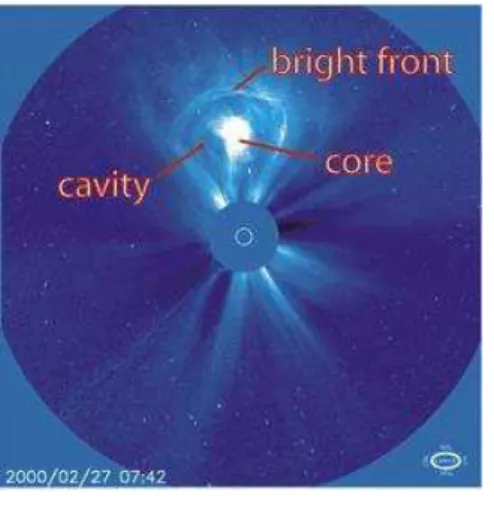
Usually CMEs present an internal structure that can be divided into three parts. From the outermost to the innermost feature, we find: a bright circular edge, called

leading edgeor bright front, which surrounds a dark region (the cavity), that contains

a brilliant eruptive prominence, that represents the bright core (see Figure4.1) (Low,

1984; Low, 1990; Hundhausen et al.,1984). CMEs may also exhibit more complex structures (Pick,2006) or can be without the circular edge, as is the case of the narrow CMEs, which are characterized by a jet-like structure along open magnetic field lines. Sometimes CMEs can occur in close succession, giving rise to the so-called multi-ple coronal mass ejectionswhose genesis in an asymmetric coronal field configuration has been studied byBemporad et al.(2012).

(37)

Chapter 4. Coronal Mass Ejection: observations and models 31

FIGURE4.1: Example of a CME showing the bright front (or leading edge), the cavity and the core. The CME was observed by LASCO–C3

coronagraph onboard of SOHO spacecraft (Riley et al.,2008)

.

Sheeley et al.(1999) classified the CMEs, directed approximately along the line of sight (LOS), in two different classes depending on whether their height/time pro-files increase or decrease: the gradually accelerating CMEs and the fast decelerating CMEs.

The core and the leading edges of the gradually accelerating CMEs are charac-terized by an almost constant acceleration, ranging between 8 and 40 m s−2, and

reach speeds of 600 to 1300 km s−1 (Sheeley et al.,1999). When gradually

accelerat-ing CMEs are observed along the LOS, they are generally seen as regular halos that surround the coronagraph disk. Away from the Sun, gradually accelerating CMEs slowly disappear reaching a constant velocity. Some gradual CMEs that are Earth directed are associated to geomagnetic storms and interplanetary shocks.

Impulsive CMEs, or fast decelerating events, are often associated with flares and Moreton waves (impulsive disturbances observed in the wings of the Hα line, prop-agating at speeds ranging from 102

to 103

km/sec) occurring on the visible disk of the Sun. They are characterized by a velocity higher than 750 km s−1 and show

irregular leading edges with a high ragged fine structure. They show a high decel-eration and in 1 hour they reduce their velocities from 1000 to 500 km s−1. Examples

of gradual and impulsive CMEs are shown in Figure4.2.

Figure4.3reports a sequence of images showing the evolution of a CMEs char-acterized by an angular width greater than 120◦.The coronal image shown in Figure

4.4, (top panel) exhibits a CME occurring on the backside of the Sun, that does not present a component able to hit the Earth. Figure4.4, (bottom panel) shows a CME occurring on the visible side of the Sun.

4.2 Models for CMEs initiation

Several models have been proposed to explain the initiation of CMEs. Usually in these models the pre-eruption state of the coronal magnetic field is stressed beyond

(38)

FIGURE4.2: Left: Gradual CMEs. Right: Impulsive CMEs.

its minimum energy configuration and the magnetic field is in a force-free field con-figuration.

In the following we present a brief overview of these models.

The thermal blast model: First CME models were based on the hypothesis that

the increase of thermal pressure gradient produced by a flare in a stressed magnetic field could be the cause of their occurrence. This phenomenon is similar to the over-lying pressure created by a bomb (Dryer,1982andWu,1982). However, it is now well known from the observations that there are many CMEs not associated with flares and others that are followed by flares (Gosling,1993). A schematic cartoon of this model is shown in Figure4.5.

The mass loading model: In this model a mass located in chromosphere or

corona, represented by a large filament/prominence, exerts its weight on a magnetic arcade, stressing the magnetic field lines as a compress spring. A CME occurs when the mass slips off, releasing the stressed magnetic field lines, as could occur in a spring without weight on it. A schematic view of this model is shown in Figure4.6.

The Tether Release, Tether Cutting and flux cancellation models: The Tether

Release Model takes into account a possible break of the equilibrium between the magnetic tension (downward) and magnetic pressure (upward) in a magnetic ar-cade. The magnetic field lines that provide the magnetic tension are called tethers. This model can be sketched with many ropes that compress a spring and a mass over the spring. When these ropes are released or they are cut, the tension of the system above the spring increases. After a certain period of time, the spring becomes unable to keep its position and then, it releases the mass abruptly causing a CME eruption. The main difference between the tether cutting and the tether release model is that in the latter the stress on the tethers gradually increases because of external forces which will cause it to break. van Ballegooijen and Martens(1989) pointed out that the cancellation of magnetic flux near the neutral line of a sheared magnetic arcade would produce helical magnetic field lines, i.e., flux ropes. This configuration can support a filament, but if magnetic flux cancellation takes place, the filament can be erupted, giving rise to a CME. It is worthwhile to stress that the tether cutting and the flux cancellation models are quite similar, being both based on reconnection, but while the latter is related to a more gradual evolution occurring in the photosphere, the former is more impulsive and occurs in the low corona. A schematic view of

(39)

FIGURE4.3: Example of a partial halo CME evolution observed the 1st Jan 2014 using the LASCO–C3 coronagraph onboard of SOHO spacecraft. The event started at 14:00 UT and ended at 19:15 UT. Note that a partial halo CME during its eruption does not cover the whole

coronagraph disk.

these models is shown in Figure4.7.

The Breakout model: The Magnetic Breakout Model, proposed by (Antiochos,

DeVore, and Klimchuk,1999) is based on a multipolar magnetic field configuration, where a slow and gradual reconnection at a neutral point between a sheared arcade and neighboring flux systems triggers the eruption. A schematic view of this model is shown in figure4.8.

(40)

FIGURE4.4: Top: Example of Backside CME. Bottom: Frontside halo CME observed the 22th June 2015 at 18:24 UT. This event is associated

with two flares of class M2.0 and M2.6 respectively.

FIGURE4.5: Thermal blast model evolution (Aschwanden,2005)

.

FIGURE4.6: Mass loading model evolution (Aschwanden,2005)

.

The flux rope model: In this model the initiation of the CME consists of two

(41)

FIGURE4.7: Tether release (left panel) and tether cutting (right panel) models evolution (Aschwanden,2005)

.

FIGURE 4.8: Breakout model. The magnetic reconnection at a neu-tral point removes the constraint over the flux rope and allows the

eruption (Antiochos, DeVore, and Klimchuk(1999))

.

twisted flux tube. The pre-eruption configuration consists of an infinitely long flux rope and an overlying arcade. When the flux rope starts to rise, the magnetic field lines will reconnect below it, forming some magnetic islands (Forbes, and Isenberg,

1991).

The Flux injection model: In this model the destabilization of the magnetic field

is caused by fast footpoint shearing motion, giving rise to an increase of the stored magnetic energy. In particular, the mechanism called flux injection occurs when the magnetic field footpoints remain anchored in photosphere and new magnetic flux emerges (Krall, Chen, and Santoro,2000).

4.3 The state-of-the-art on statistical studies of CMEs

param-eters

Ivanov and Obridko(2001) carried out an analysis on the semi-annual mean CMEs velocities in the time window 1979 – 1989 and they found a complex cyclic variation that presents two peaks. The first one is located at the maximum of the solar cycle. The second one, called secondary, is present at the solar cycle minimum.Ivanov and

(42)

Obridko (2001) stated that the peak at the minimum of solar cycle in a time win-dow ranging from 1985 – 1986 could be attributed to the conspicuous contribution of fast CMEs that have an angular width around 100◦at solar cycle minimum. This

significant contribution leads to an increase of the global magnetic field observed at large scale in our Sun. Moreover, they highlighted that on average, an increase of the velocity always provokes the growth of the CMEs width.

More recently,Mittal et al.(2009a) reported on the analysis of more than 12900 CMEs observed by the LASCO coronagraph onboard SOHO in the time interval 1996 – 2007. Their results indicate a decrease in the velocity in the descending part of Solar Cycle 23. In the year 2001 was observed an unexpected decrease in the velocities of the CMEs and a peak, that corresponds to the Halloween events in 2003, where many CMEs, flares of X class, shocks and Solar Energetic Particles (SEP) events were observed in October and November 2003.

Using the same dataset, Mittal and Narain (2009b) found that the majority of CMEs (66 %) present negative acceleration, while the CMEs with positive acceler-ation are the 25 % and the other showed a lower acceleracceler-ation (9 %) in the external coronal layer.

Cremades and St. Cyr(2007) studied the latitudes of CMEs using a wide sample, since 1980 up to 2005, in order to investigate the possible matches between CMEs and coronal streamers location. They found a good correlation, in agreement with

Hundhausen(1993) (see alsoGopalswamy et al.,2004).

All these studies have allowed significant steps forward in the comprehension of the CMEs properties, but there are still several open issues, like for instance a clear explanation of why CMEs can have different velocities and acceleration regimes, the reasons of the observed variation of these parameters along the solar cycle, why some CMEs are clearly correlated with flares while others do not seem to show any correlation.

The following Chapters 5 and 6 will describe the research carried out in this The-sis in order to provide a further contribution to the solution of these open problems.

(43)

37

Chapter 5

Statistical analysis on selected

CME’s parameters

This chapter reports a statistical study of some CMEs parameters and their variation over the Solar Cycles 23 and 24 (Compagnino et al.,2017).

5.1 LASCO and CACTus datasets

The CMEs data analyzed in this thesis were acquired by the LASCO C2 and C3 coro-nagraphs onboard the SOHO satellite in a time interval extending for 18 years, from 31 July 1996 to 31 March 2014. We used two different datasets: the former obtained from the Coordinated Data Analysis Workshops (CDAW) Data Center online CME catalog, available at the following link: cdaw.gsfc.nasa.gov/CME_listand the latter

through the Computer Aided CME Tracking software (CACTus) available at the fol-lowing link: sidc.oma.be/cactus/. Using two different catalogs we could compare

the results obtained through the manual identification method for CMEs detection (CDAW) with the automated identification by CMEs tracking (CACTus).

The CDAW catalog includes information about several CMEs parameters: the polar angle (PA) i.e., the mean angle within the two external edges of the CME width measured in degree on the plane of the sky counterclockwise from the North direc-tion, the linear velocity, the acceleradirec-tion, the width, the mass and the energy of the CMEs. Some of these parameters are also reported in the CACTus dataset, which however does not contain information about the CMEs mass, energy and accelera-tion. It is worth noting that the CME start time recorded in these datasets indicates the first CME detection in the LASCO C2 Field of View (FOV), i.e the region rang-ing from about 2.0 to 6.0 solar radius. The events in the CDAW catalog are 22876 (616 halo CMEs, i.e. 2.69 % of all CMEs), while the events in the CACTus catalog are 15515.

5.2 CME Parameters Over the Solar Cycles 23 and 24

The annual CMEs occurrence during the solar cycle 23 and 24 is shown in Figure5.1

(the black line represents the CACTus data, while the dot–dashed blue lines repre-sents the CDAW data).

(44)

Chapter 5. Statistical analysis on selected CME’s parameters 38

FIGURE 5.1: Number of observed CMEs for each year observed in the considered time widow for CDAW (black line) and CACTus (dot– dashed-blue lines). The yearly Wolf Number is marked by

long-dashed-red line

.

We observe two sharp peaks referred to the maxima of the solar cycles 23 and 24. We note that the analysis carried out using the CDAW dataset shows a higher peak related to the occurrence of the CMEs in the cycle 24. This behaviour seems to be in contrast with the weaker magnetic activity observed during the current solar cycle than in solar cycle 23, as already noted byTripathy, Jain, and Hill(2015), and shown in Figure5.1 by the yearly Wolf number (long-dashed-red line). As mentioned in the analysis and measurement of the acoustic solar modes frequency shifts in the two cycles carried out by Tripathy, Jain, and Hill(2015) the weakness of the peak in the solar cycle 24 may be attributed to faint polar field strength observed in solar cycle 23. A very low solar magnetic field during the cycle 24 is also documented by the sunspot number (SSN). This activity is the lowest recorded from the space age inception until now and several authors make the hypothesis of a global minimum in solar cycle 24 (Padmanabhan et al.,2015;Zolotova and Ponyavin,2014).

Moreover, using the CMEs detected by CACTus we note that the number of CMEs occurred each year (N) is of the same order of magnitude during the peaks of the two cycles, and that the peak of CME distribution during the Cycle 24 is more extended in time ( N > 1500 during 2012 and 2013). Another important conclusion is that the differences between CDAW and CACTus may be due to different CME definition in the CDAW catalog that lead to an observed bias in CMEs detection (Robbrecht, Berghmans, and Van der Linden,2009;Webb and Howard,2012;Yashiro, Michalek, and Gopalswamy,2008).

In Figure5.2(from top to bottom) we show the behavior of the average annual velocity, acceleration and angular width for all the observed CMEs during the Solar Cycles 23 and 24. For the velocity and the angular width we plot the results of CDAW dataset (black line) and of CACTus dataset (dot–dashed-blue line), while for the acceleration we show only the CDAW results because this parameter is not available in the CACTus dataset. The blue diamonds indicate the CACTus data.

(45)

FIGURE 5.2: Mean CME velocity distribution for each year (top panel), acceleration (middle panel,) and angular width (bottom panel) in a period that covers the time window between 1996 and 2014. The results for CDAW are indicated by a black line, while for CACTus dataset dot–dashed-blue lines are used. In each panel the yearly Wolf Number is marked by long-dashed-red line. The

(46)

of CMEs for each year and then considering the velocity averaged with respect to this number. The same procedure was applied for the other parameters. We also computed the error bars for the mean distribution of these quantities, as σ/√N, where σ is the standard deviation of the corresponding quantity and N is the number of CMEs that occurred in each year (see Aarnio et al. (2011)). The error bars are smaller than the symbol sizes, although the error for the acceleration is dominated by the uncertainty of the individual measurements. The red line in each panel shows the yearly Wolf number. For the average velocity we can see a first peak around 2003 and a second one between 2012 and 2014 in both of the datasets.

The behaviour of both of the datasets reflects the solar-activity cycles and can be interpreted according toQiu and Yurchyshyn(2005) as an effect of the magnetic flux involved by the events during the solar maxima. However, one difference between the two datasets is that in the mean-velocity distribution of the CMEs detected by CACTus there is another peak between 2008 and 2010, during the minimum of the solar cycle. A secondary peak was reported byIvanov and Obridko(2001) from the analysis of CMEs velocities for the time interval 1979 – 1989, and was interpreted by these authors as due to a significant contribution of fast CMEs (V > 400 km s−1)

with a width of 100◦.

The mean CMEs acceleration for CDAW is 3.2± 0.3 m s−2. In the distribution of

the CME average acceleration (middle panel of Figure5.2) we see negative values around the maximum of Solar Cycle 23 and a peculiar peak of about 15± 3 m s−2in

2009. We note that this peak occurs approximately when we observe the minimum in the annual average velocity distribution for CDAW and the second peak of the velocity distribution for CACTus. However, statistically the slower CMEs occurring during solar-activity minimum, are characterized by higher positive values of accel-eration.

In Figure5.2( bottom panel), showing the mean angular width, the values in the years 2000 – 2003 for CDAW dataset (≈ 20◦) suggest that on average the narrowest

CMEs are the slowest ones (compare with Figure5.2(top panel)) (Yashiro, Michalek, and Gopalswamy,2008). We also note that for the CACTus dataset the fastest CMEs are the narrowest (Yashiro, Michalek, and Gopalswamy,2008). Both datasets show a minimum in the mean width distribution over the years corresponding to the min-imum of the solar cycle, althoughYashiro, Michalek, and Gopalswamy(2008) found that the CACTus catalog has a larger number of narrow CMEs than CDAW. This dif-ference in the two samples determines a different amplitude in the range spanned by the mean angular width distribution, i.e. in the CACTus catalog the mean width varies from ≈ 30◦ during the minimum of solar-activity to ≈ 40◦ during the

maxi-mum of activity, while for CDAW catalog varies between ≈ 20◦ and ≈ 80◦.

In order to further analyze the properties of CMEs during the descending part of the Solar Cycle 23, in Figures5.3, 5.4, and 5.5 we show the distribution of the velocity, acceleration and width of the CMEs for each year from 2000 to 2006.

Figure5.3shows that the tail of the distribution of the CME velocity observed during the descending part of the solar cycle 23 decreases from the maximum (2000) to the minimum (2006) of the cycle. This means that most of the fastest CMEs veloci-ties (> 1000 km s−1) occur during the maximum of the solar cycle, when the amount

Properties and correlation of flares and coronal mass ejections and their possible relevance on the southern night sky background: a statistical study

UNIVERSITÀ DEGLI STUDI DI CATANIA

P

ROPERTIES AND CORRELATION OF

FLARES AND CORONAL MASS EJECTIONS

AND THEIR POSSIBLE RELEVANCE ON THE

SOUTHERN NIGHT SKY BACKGROUND

:

A

STATISTICAL STUDY

Contents

Abstract

Chapter 1

Introduction

1.1

Eruptive phenomena on the Sun

1.2

Effects of solar phenomena on the Earth environment

Chapter 2

Solar flares: observational

characteristics and standard model

2.1

Flare emission, morphology, physical parameters

2.2

Flare classifications

2.3

Standard model

Chapter 3

Flare occurrence in Active

Longitudes

3.1

Data sample

3.2

Flare Distribution Over the Solar Cycles

3.3

Results of the analysis on flare occurrence in Active

Lon-gitudes

3.4

Summary

Chapter 4

Coronal Mass Ejection:

observations and models

4.1

CME morphology and physical parameters

4.2

Models for CMEs initiation

4.3

The state-of-the-art on statistical studies of CMEs

param-eters

Chapter 5

Statistical analysis on selected

CME’s parameters

5.1

LASCO and CACTus datasets

5.2

CME Parameters Over the Solar Cycles 23 and 24