An Instrumental Variable Probit (IVP) analysis on depressed mood in Korea: the impact of gender differences and other socio-economic factors

(1)

An Instrumental Variable Probit (IVP) analysis on

depressed mood in Korea: the impact of gender differences

and other socio-economic factors

Lara Gitto1*_{, Yong-Hwan Noh}2_{, Antonio Rodríguez Andrés}3 Abstract

Background: Depression is a mental health state whose frequency has been increasing in modern societies. It imposes a great burden, because of the strong impact on people’s quality of life and happiness. Depression can be reliably diagnosed and treated in primary care: if more people could get effective treatments earlier, the costs related to depression would be reversed. The aim of this study was to examine the influence of socio-economic factors and gender on depressed mood, focusing on Korea. In fact, in spite of the great amount of empirical studies carried out for other countries, few epidemiological studies have examined the socio-economic determinants of depression in Korea and they were either limited to samples of employed women or did not control for individual health status. Moreover, as the likely data endogeneity (i.e. the possibility of correlation between the dependent variable and the error term as a result of autocorrelation or simultaneity, such as, in this case, the depressed mood due to health factors that, in turn might be caused by depression), might bias the results, the present study proposes an empirical approach, based on instrumental variables, to deal with this problem.

Methods: Data for the year 2008 from the Korea National Health and Nutrition Examination Survey (KNHANES) were employed. About seven thousands of people (N= 6,751, of which 43% were males and 57% females), aged from 19 to 75 years old, were included in the sample considered in the analysis. In order to take into account the possible endogeneity of some explanatory variables, two Instrumental Variables Probit (IVP) regressions were estimated; the variables for which instrumental equations were estimated were related to the participation of women to the workforce and to good health, as reported by people in the sample. Explanatory variables were related to age, gender, family factors (such as the number of family members and marital status) and socio-economic factors (such as education, residence in metropolitan areas, and so on). As the results of the Wald test carried out after the estimations did not allow to reject the null hypothesis of endogeneity, a probit model was run too.

Results: Overall, women tend to develop depression more frequently than men. There is an inverse effect of education on depressed mood (probability of -24.6% to report a depressed mood due to high school education, as it emerges from the probit model marginal effects), while marital status and the number of family members may act as protective factors (probability to report a depressed mood of -1.0% for each family member). Depression is significantly associated with socio-economic conditions, such as work and income. Living in metropolitan areas is inversely correlated with depression (probability of -4.1% to report a depressed mood estimated through the probit model): this could be explained considering that, in rural areas, people rarely have immediate access to high-quality health services.

Conclusion: This study outlines the factors that are more likely to impact on depression, and applies an IVP model to take into account the potential endogeneity of some of the predictors of depressive mood, such as female participation to workforce and health status. A probit model has been estimated too. Depression is associated with a wide range of socio-economic factors, although the strength and direction of the association can differ by gender. Prevention approaches to contrast depressive symptoms might take into consideration the evidence offered by the present study.

Citation: Gitto L, Noh YH, Andrés AR. An Instrumental Variable Probit (IVP) analysis on depressed mood in Korea: the impact of gender differences and other socio-economic factors. Int J Health Policy Manag 2015; 4: x–x. doi: 10.15171/ijhpm.2015.82 *Correspondence to: Lara Gitto Email: Gitto@CEIS.uniroma2.it Article History: Received: 26 September 2014 Accepted: 7 April 2015 ePublished: 16 April 2015

Original Article

Int J Health Policy Manag 2015, 4(x), 1–8 doi10.15171/ijhpm.2015.82

Implications for policy makers

• The results of the paper assist in recognizing which people are more likely to develop depression and the impact of gender differences and education level: these factors should be taken into account when assessing the benefits that could be obtained from support and counseling programs. • Being aware of the social impact of depression outlines the relevance of investing in the implementation of counseling programs. Counseling programs

and other public health measures against depression are less expensive than costs of depression.

• There is the need to monitor mental illness in rural areas too, especially where there are huge differences between urban and rural areas development, as in Korea.

Implications for public

Depression is likely to strike a large fraction of the population and support and counseling programs should be easily implemented and accessed. Support programs should be easily accessed in rural areas too, to guarantee equality of treatment for mental illness.

(2)

Background

Mental health disorders, among these ones, depression, are likely to impose a great burden in modern societies (1). Depression brings about the human costs of sadness, sense of isolation, inability to enjoy life, and, for 35,000 people every year, attempted suicide (2). Depressed individuals are five times more likely to abuse drugs (3,4).

In addition to human costs, economic costs have to be taken into account too: people lose 5.6 hours of productive work every week when they are depressed (5): it has been estimated how half of the loss of work productivity is due to absenteeism and short-term disability (6,7). People with symptoms of depression are 2.17 times more likely to take sick days (8) and, when they are at work, their productivity is impaired, depending on how severe the depression is. Workplace costs of depression have been estimated being over $34 billion per year (9); as the costs of absenteeism were directly related to actually taking antidepressant medications (10), those people who took the prescribed medication had a 20% lower cost of absenteeism.

Lastly, it is well-documented that poor mental health contributes to unemployment. The unemployed tend to have higher levels of impaired mental health, including anxiety, depression, as well as higher levels of mental health hospital admission, premature mortality, and chronic diseases (11). If people showing affective symptoms and depression seek treatment earlier – and get effective treatment – the human cost and the economic costs could be reversed (3).

Depression is a disorder that can be reliably diagnosed and treated in primary care: as outlined in the World Health Organization (WHO) mhGAP Intervention Guide (12), preferable treatment options consist of basic psychosocial support combined with antidepressant medication or psychotherapy, such as cognitive behavior therapy, interpersonal psychotherapy or problem-solving treatment. Looking at gender, depression also strikes more women than men: its prevalence is one to five times greater in females (13–19). This gender gap can be explained by genetic, neuro-hormonal, psychobiological (20) and social factors (21), the latter far more predictive of gender gaps in depression than genetic or hormonal factors.

Gender gaps have been seen identified in the formal literature when considering men’s lower likelihood to seek care; in a recent study, it has been observed that the circumstance of women having a higher care use is dependent on the type of care provider, with greater gender inequality in the use of primary healthcare (22). Further, women might be more likely to experience both role and financial strains, that may be associated, for example with child care difficulties, the need to juggle work and family responsibilities, and single parenthood (23–25).

This study focuses on the individual determinants of depressive behavior and its gender differences using data from South Korea. Few epidemiological studies have examined the determinants of depression in Korea so far, and they were either limited to samples of employed women or did not control for individual health status (26–29). Former research reported the prevalence of depression disorders in several world regions, but Korean statistics were not mentioned. In the geographic region including Eastern Asian countries as

China and Vietnam, people aged 19–79 experiencing at least 10 depression episodes ranged between 18.5% and 24%. In South Eastern Asia (such as Thailand, Indonesia, etc.) this percentage was lower and ranged between 13% and 18% (30). The choice of covariates to include in the analysis was based on previous empirical studies on depression.

In addition to gender, age is among determinants of depressed mood (31,32). Empirical analyses have sometimes revealed a modest effect of age on mental health (33), sometimes no evidence at all that depression increases with age (34) and other times a strong association between age and the prevalence of symptoms of depression (35). In this paper, to account for a non-linear association between age and depression, age and age-squared were included in the empirical model (19).

The positive association between social relationships and health has been stressed in many studies: a pioneering study considers social relationships as a risk factor for health, including in a wide notion of health, mental health too (36). Depression can be correlated with household size and income. Household size is a proxy for family support, which is expected to influence respondents’ psychological well-being. It has been seen how the frequency of affective symptoms is lower in large families, although it is higher when the household income is low (37–39)1_.

A number of studies also control for marital status. Marriage can act as a protective factor against the occurrence of depression (40,41). Depression is more common among non-married, single, divorced, and, especially, widows (33). A dummy variable was employed in the estimations by marital status, assuming a value of 1 if the respondent was married and 0 otherwise.

To our knowledge, living in urban areas as source of depression has been neglected in the empirical literature on depression. In Korea, metropolitan areas are more densely populated than in any other countries.

To control for regional heterogeneity lifestyles and environmental conditions on depression, a regional dummy representing residents in metropolitan areas (including Seoul, Incheon and Gyeonggi-do) was included. In fact, these areas are more densely populated than in any other countries. As a quick example, 25,620,000 people, who constitute the 49.5% of Korean population, live in an area of 11,806 squared-km, which represents the 11.8% of the whole country2_.

As a result, while the largest towns might face higher congestion costs than those of rural areas, their residents have immediate access to higher quality services. Moreover, Korea also faces inequality issues, as productive activities are highly concentrated in metropolitan areas.

Physical illness should also be considered (25), since depression often occurs with other comorbidity factors (42). Poor physical health might lead to depression in later stages of life (43). Here, health status is assessed by the following question in the survey: “How is your health in general: would you say it is…?” The available answers, measured on a Likert scale, were: “very good”= 1, “good”= 2, “not bad”= 3, “bad”= 4 “very bad”= 5. Other indicators for people’s health were the results of blood tests, blood pressure, and some individual habits, such as smoking.

(3)

problems of endogeneity. Depression might depend on the fact that individuals experience a poor level of health and vice

versa (i.e. poor health is determined by a depressed mood that

does not allow individuals to take care of themselves). Other socio-economic variables that might be considered as determinants of depression are likely to be endogenous. High frequencies of mental disorders are connected with low education (44,45), family income, as it has been already stressed (18,46) and participation in the workforce (47), especially for women. To account for labor market status, a dummy variable assuming a value of 1 if the respondent was an employed woman and 0 otherwise was included as a regressor.

In order to address the endogeneity biases, two Instrumental Variables Probit (IVP) models were estimated, using as instruments: 1) the average income for workers and education level (college and high school) in the first model, that considered female workforce participation as an endogenous variable; and 2) the results of blood analysis (anemia, level of cholesterol, level of glucose), blood pressure and smoking in the second model, where the circumstance of reporting a good level of health was the variable suspected to be endogenous. The hypothesis tested concerns the existence of gender differences in reporting depressed mood; females are more likely to declare such symptoms, but family factors, and workforce participation should counteract this tendency. The paper is organized as follows: the next section, dedicated to methods, describes the IVP model, the data employed and the variables selected; results of the estimations are presented in the following section. Comments on the results and implications for health policies conclude the study.

Methods

The statistical model (IVP)

The first empirical model estimated in this study can be formalized as follows:

y_i= a_i + bX’_i + u_i (1)

Y is the dependent binary variable (depression yes/no); α is

the constant term; β is a k × 1 vector, X is an n × k matrix of covariates; u is the error term.

However, the probit model can be biased because of endogeneity. In this case, the correlation between the regressors and the error term is not zero (E (X, u) ≠ 0), so that the results of the estimation are inconsistent (48). One way to overcome this issue is to apply instrumental variables.

The above model can be written in its reduced form:

y*_1i = βy_2i + γx_1i + u_i (2a)

y_2i = x_1i Π₁ + x_2i Π₂ + v_i (2b) Here y*_1i is the dependent variable for the ith observation (i.e. the answer to the question, “Do you currently have chronic depression?”)3_.

Depression, as proxied in this paper, may not represent the true value of such condition: in fact, a self-reported measure might pick up cultural differences in the description of subjective feelings and may be influenced by time and other factors occurring when the interview was done.

However, self-report depression measures are becoming increasingly important (50); then, they can be easily

implemented to large samples (51,52).

In (2a), y_2i is a vector of endogenous variables (in our case, the female workforce participation and the circumstance to report a good level for health); x_1i and x_2i are, respectively, a vector of exogenous regressors and variables used as “instruments”; β and γ are vectors of other structural parameters.

In (2b), Π₁and Π₂are matrices of parameters. By assumption, (u_i, v_i) ~ N (0, Σ).

The estimation of the endogenous probit model can be done through a two-step procedure, such as the one proposed by Newey (53,54). Stata software package Version 10.0, which has been employed for the estimations, performs MLE (55). Regarding the selection of variables to use as suitable instruments, when panel data are available, a good option could be employing the first lag for all potentially endogenous variables, as lags can offer consistent estimators of the coefficient of interest (54). However, this is not the case here, as cross-sectional data are employed.

Sample selection

The Korea National Health and Nutrition Examination Survey (KNHANES) was employed in the analysis. The KNHANES is a population-based cross-sectional survey designed to assess the health-related behavior, health condition, and nutritional state of Koreans. Beginning with the forth wave in 2007, it was converted to an annual survey. The KNHANES provides a rich source of data and its participants are representative of the Korean population. In the last decade, the database has been increasingly employed in medical and epidemiological studies4_.

The data used in this study is from 2008 and information was gathered via face-to-face interviews. This analysis was restricted to respondents aged 19–75 years. Respondents younger than 19 years old or older than 75 years old were excluded as they are more likely to develop depression due to hormonal shifts in puberty and sickness at old age, so that the above circumstances may have biased the results.

Hence, the final sample considered for this study included 6,751 respondents out of total of 9,744 observations.

Measures

Some information contained in the KNHANES, related to residence, work and people’s health have been selected for the empirical analysis.

The variables employed related to individuals’ age and age squared, gender, marital status, number of family members, residence in metropolitan areas, female participation to workforce (a dummy variable assuming value= 1 if the respondent is a woman currently employed and= 0 otherwise), average income for workers and educational level.

Variables related to health were high blood pressure (a dummy variable assuming value= 1 if people had systolic blood pressure higher than 140 and= 0 otherwise), the level of hemoglobin (anemia), the level of cholesterol in the blood (cholesterol), the level of glucose in the blood (glucose), the circumstance to be a smoker.

We did run two estimations of the IVP model. In the first one, we considered the effect of socio-economic variables, such as the circumstance of living in metropolitan areas, the

(4)

average income of workers, and the level of education, which is likely to determine women’s participation in the workforce. In the second estimation, attention was paid to a satisfactory level of health (a dichotomous variable assuming a value of 1 if the reported health status on a Likert scale was ≥3 on a scale 0–5 and 0 otherwise). “Good health” was measured by considering clinical parameters as the level of blood pressure, the presence of anemia, the levels of cholesterol and glucose in blood tests, and the circumstance of being a smoker. After the estimation, Wald tests for exogeneity were conducted in order to control if IVP regression might be a suitable approach. If it is not possible to reject the null hypothesis of exogeneity, there is no need for an IVP approach and estimates of a probit model are more efficient.

Results

Table 1 and 2 display descriptive statistics of the all variables

included in the empirical analysis.

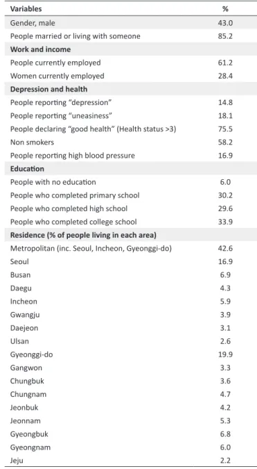
Forty-three percent of people in the sample were male; more than eighty-five percent were married or lived with someone, while 61.2% were currently employed. There are gender differences in the level of salary (106.1 (10,000 KRW) for male workers vs. 78.2 (10,000 KRW) for female workers as average monthly salary). Women’s workforce participation is also limited (28.4% of women were included in the sample). About 34% of people in the sample completed college education. More than 42.0% live in metropolitan areas: Seoul and Gyeonggi-do are the most populated regions.

More than 75.0% of people declared to be in good health; almost 15.0% of the sample population answered positively when asked about depressed mood. As expected, a higher percentage of women reported depression compared to men, although this measure is not a clinical diagnosis of depression but rather a subjective one5_.

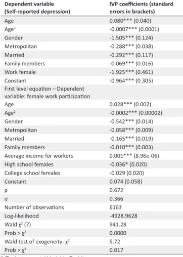
The results of the IVP estimation after controlling for the potential endogeneity of work female are reported in Table 3. Marginal effects are reported in Table 4.

The estimated probability of reporting depression is 19.7%. It is possible to see a huge difference across gender: the estimated probability of women reporting depression is 37.2% higher than for males.

Table 1. Descriptive statistics (KHNANES, forth wave, N= 6,751

respondents) - Mean

Variables Mean SD Min. Max.

Age (between 19 and 75) 46.8 15.1 19 75

Number of family members 3.4 1.4 1 10

Work and income

Average household monthly

income (10,000 KRW) 184.3 532.6 0 25,000

Monthly income for female

workers (10,000 KRW) 78.2 365.6 0 25,000

Monthly income for male

workers (10,000 KRW) 106.1 408.1 0 25,000

Depression and health

Health status (Likert scale) 2.8 0.9 1 5

Cholesterol (mg/dL) 187.2 35.9 0 1

Glucose (mg/dL) 98.2 24.7 43 642

Anemia (dummy) 0.1 0.3 0 1

KHNANES= Korea National Health and Nutrition Examination Survey.

Table 2. Descriptive statistics (KHNANES, forth wave, N= 6,751

respondents) - Percentages

Variables %

Gender, male 43.0

People married or living with someone 85.2

Work and income

People currently employed 61.2

Women currently employed 28.4

Depression and health

People reporting “depression” 14.8

People reporting “uneasiness” 18.1

People declaring “good health” (Health status >3) 75.5

Non smokers 58.2

People reporting high blood pressure 16.9

Education

People with no education 6.0

People who completed primary school 30.2

People who completed high school 29.6

People who completed college school 33.9

Residence (% of people living in each area)

Metropolitan (inc. Seoul, Incheon, Gyeonggi-do) 42.6

Seoul 16.9 Busan 6.9 Daegu 4.3 Incheon 5.9 Gwangju 3.9 Daejeon 3.1 Ulsan 2.6 Gyeonggi-do 19.9 Gangwon 3.3 Chungbuk 3.6 Chungnam 4.7 Jeonbuk 4.2 Jeonnam 5.3 Gyeongbuk 6.8 Gyeongnam 6.0 Jeju 2.2

In a second equation, the focus was on variables related to health. “Good health”, that assumes a value of 1 if a score higher than 3 about health status is reported and 0 otherwise, is the variable for which an instrumental equation has been estimated. Instruments are related to individuals’ habits (being a smoker or not) and clinical conditions (blood pressure, anemia, cholesterol and glucose).

Results of the estimations are reported in Table 5. The estimated coefficients are smaller, as for the number of family members, while variables related to education are not significantly estimated. As a robustness check, we tested the exogeneity of the variables included in our empirical specification. For that purpose, an instrumental variables approach was carried out.

Since the results of the Wald test do not allow to reject the null hypothesis, a probit model was run, performing the link test for model specification after the estimation.

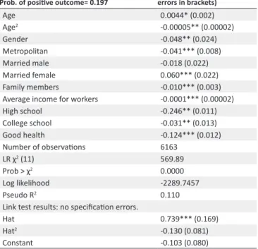
Table 6 displays the marginal effects of the probit model.

(5)

signs and significance of the IVP.

Again, higher education and college education are significantly and inversely correlated with the dependent variable and show how the probability of reporting depressed mood is of -24.6% for people who completed high school and of -3.1% for those ones graduated at college. The probability to report depression diminishes to 12.4% when good health (score >3 on a Likert scale) is overall reported.

Discussion

The empirical results are in line with previous empirical literature on the determinants of self-reported depression. Overall, women tend to experience depression more often than men. Being married and socio-economic factors were found to be protective factors against depression.

Table 3. IVP regression (1) with the variable “work female”

Dependent variable

(Self-reported depression) IVP coefficients (standard errors in brackets)

Age 0.080*** (0.040) Age2 _{-0.0007*** (0.0001)} Gender -1.505*** (0.124) Metropolitan -0.288*** (0.038) Married -0.292*** (0.117) Family members -0.069*** (0.016) Work female -1.925*** (0.461) Constant -0.964*** (0.305)

First level equation – Dependent variable: female work participation

Age 0.028*** (0.002) Age2 _{-0.0002*** (0.00002)} Gender -0.542*** (0.014) Metropolitan -0.058*** (0.009) Married -0.165*** (0.019) Family members -0.010*** (0.003)

Average income for workers 0.001*** (8.96e-06) High school females -0.036* (0.020) College school females -0.029 (0.020)

Constant 0.074 (0.058) ρ 0.672 σ 0.366 Number of observations 6163 Log-likelihood -4928.9628 Wald χ2₍₇₎ _941.28 Prob > χ2 _0.0000

Wald test of exogeneity: χ2 _5.72

Prob > χ2 _0.017

IVP= Instrumental Variable Probit.

*** significant at 99%; ** _{significant at 95%; *} _{significant at 90%.}

Table 4. Marginal effects of IVP (1) Dependent variable (Self-reported depression) Prob of positive outcome= 0.197

IVP coefficients (standard errors in brackets) Age 0.022*** (0.006) Age2 _{-0.0002*** (0.00007)} Gender -0.372*** (0.083) Metropolitan -0.071*** (0.013) Married -0.088* (0.048) Family members -0.019*** (0.048) Work female -0.369*** (0.128)

Table 5. IVP regression (2) with the variable: “good health”

Dependent variable

(Self-reported depression) IVP coefficients(standard errors in brackets)

Age 0.024** (0.012) Age2 _{-0.0003*** (0.0001)} Gender -0.532*** (0.084) Metropolitan -0.205*** (0.048) Married 0.153 (0.94) Family members -0.038** (0.018)

Average income for workers -0.0004*** (0.0001)

College school -0.084 (0.104)

High school -0.045 (0.0909

Good health -1.121** (0.477)

Constant -0.260 (0.456)

First level equation - Dependent variable: Good health

Age 0.001 (0.003) Age2 _{-0.0005*** (0.00002)} Gender 0.130*** (0.015) Metropolitan 0.013 (0.015) Married 0.043** (0.021) Family members 0.012*** (0.004)

Average income for workers 0.00001* (9.93e-06)

High school 0.119*** (0.016)

College school 0.131*** (0.018)

High blood pressure 0.004 (0.013)

Anemia -0.058*** (0.018) Cholesterol 0.0003*** (0.0001) Glucose -0.001*** (0.0002) Constant 0.662*** (0.070) ρ 0.235 σ 0.401 Number of observations 5949 Log-likelihood -5233.9247 Wald χ2₍₇₎ _433.83 Prob > χ2 _0.0000

Wald test of exogeneity: χ2 _1.22

Prob > χ2 _0.268

We found a nonlinear relationship between age and depression. In particular, the estimated coefficient for age is positively and significantly correlated with depression, while a negative and significant correlation exists with the squared term, though the estimated coefficient is indeed small and shows that aging has little effect on the probability of reporting depression.

Surprisingly, living in a metropolitan area reduces the risk of experiencing depression. A potential explanation for this pattern is that living in big cities might offer better job opportunities and career advance. Indeed, women might be more vulnerable in a competitive environment than their male counterparts. However, it has been recently shown in some studies that quality of life may be higher in urban areas and that it might be more difficult to recover from depression in rural areas, especially for elderly women (57). Although urban life in Korea can be very stressful due to the working conditions (hierarchical society and poor working conditions for non-regular workers) and the high cost of living, there are more resources to explore in urban areas. In addition, some studies have outlined how chronic medical conditions are more prevalent in rural areas – a circumstance that may also

(6)

affect the overall quality of life (58,59).

The risk of depression decreases as family size increases. This result confirms the findings of the literature on self-reported happiness: it has been demonstrated that people living with their grandchildren enjoy a higher quality of life (i.e. the larger the number of family members, the higher the level of happiness) (60). Conversely, it should be possible to argue that the more people living in the same family, the lower the risk of depression.

Workforce participation, especially for women, can be influenced by several factors, mainly related to family. In the empirical estimation, we included the average income for workers that could be a potential factor that might induce a higher participation by female workers, in those cases when family income is so low that another source of income for the family is necessary.

However, the increase in women workforce participation might determine, in turn, higher difficulties in managing women roles within the family and in the working environment, increasing the risk of depression

As expected, there is a negative impact of good health on the probability of reporting depression: in fact, a level of health higher than 3 over 5 on a Likert scale is inversely related with the probability of experiencing depression.

In general, this study confirms the main results of the literature: depression is significantly associated with socio-economic conditions, such as educational attainment, work, and income.

The present analysis could be refined by trying to overcome potential bias: here, depression was detected by the answers given to the question, “Do you currently have chronic depression?”

A more detailed investigation for a selected sample might aim at collecting information on the level of depression through validated questionnaires.

This study sheds light on the frequency of depressed mood in

Table 6. Probit model: marginal effects Dependent variable (Self-reported depression) Prob. of positive outcome= 0.197

Probit coefficients (standard errors in brackets) Age 0.0044* (0.002) Age2 _{-0.00005** (0.00002)} Gender -0.048** (0.024) Metropolitan -0.041*** (0.008) Married male -0.018 (0.022) Married female 0.060*** (0.022) Family members -0.010*** (0.003)

Average income for workers -0.0001*** (0.00002)

High school -0.246** (0.011) College school -0.031** (0.013) Good health -0.124*** (0.012) Number of observations 6163 LR χ2₍₁₁₎ _569.89 Prob > χ2 _0.0000 Log likelihood -2289.7457 Pseudo R2 _0.110

Link test results: no specification errors.

Hat 0.739*** (0.169)

Hat2 _{-0.130 (0.081)}

Constant -0.103 (0.080)

the population considered. It can be a good starting point for further studies aimed at analyzing, for instance, the economic impact of depression and the possible effects of counseling and support programs directed especially to the subjects more likely to report a depressed mood in the population, as women, to help them to contrast depressive symptoms. In this perspective, there are some studies, albeit only from high-income country’s contexts, indicating cost-effective approaches for the prevention of depression across the life course (60) or estimating the effect of preventive programs for mothers in the first two years after birth (61).

The positive consequences of these programs could be evaluated both in terms of economic benefits, such as the increased productivity and the diminished consumption of drugs and antidepressants, and, more importantly, in terms of health outcomes, such as a higher quality of life.

Ethical Issues

This work was supported by a research grant from Seoul Women’s University (2015) and also approved by the ethics committee of Seoul Women’s University, Seoul, South Korea.

Competing interests

Authors declare that they have no competing interests.

Authors’ contributions

LG, YHN, and ARA were involved in the study design. LG developed the research question, performed the statistical analysis, and drafted the manuscript. YHN supervised the study design, interpretation of results and manuscript revisions. ARA contributed to the data analysis and manuscript revisions. All authors read and approved the final manuscript.

Authors’ affiliations

1_{CEIS Sanità, Università di Roma “Tor Vergata”, Roma, Italy.}2_{Department of}

Economics, Seoul Women’s University, Seoul, South Korea. 3_Departamento

de Administración de Empresas, Facultad de CC. Jurídicas y Económicas, Universidad Camilo José Cela, Villanueva de la Cañada, Madrid, Spain.

Endnotes

1. In the absence of any measurement of relationship between each individual and other household members, the ages of other family members, or the type and quality of the relationship between the individual and his/her family members, the household size might not be the best proxy for family support. A household of two adults and five pre-adolescent children would not be a support system that buffers against depression the same way that a household with four adults and three pre-adolescent children would, as, in the first case, the large number of children in the household may be a risk factor for depression. Information about family members’ age cannot be obtained from the database employed and, to our knowledge, no previous studies on this topic have specifically considered each family member’ age.

2. In the same areas, the number of enlisted firms in stock market is 1,206 (71.1%, as of 2012), for an aggregate value of enlisted stock of 1,025 trillion

KRW (86%, as of 2012) (Korean Statistical Information Service, http://kosis.kr).

3. This is said to be a recursive model, as y2i appears both in equations (2a)

and (2b). About depression, the World Mental Health Survey conducted in 17 countries found that, on average, about 1 in 20 people reported having an

episode of depression in the previous year (49).

4. In fact, the number of published studies that use the KNHANES as the primary source of data has significantly grown: there are one article in 2007, three in 2008, four in 2009, three in 2010, five in 2011, and five in 2012 which

have used the KNHANES data as their primary data source (56).

5. Looking at the KNHANES database, we noticed how another variable that could be considered as a proxy to state the presence of a depressed mood is the feeling of “uneasiness”, which represents the difficulties faced by individuals in coping with daily life. The respondents answered to the question, “Are you

(7)

having difficulty in coping with daily social life due to physical and/or mental problems?” (Yes= 1, No= 0). Overall, the feeling of uneasiness was reported by 18.1% of respondents.

References

1. Kessler RC, Aguilar-Gaxiola S, Alonso J, Chatterji S, Lee S, Ormel J, et al. The global burden of mental disorders: An update from the WHO World Mental Health (WMH) Surveys. Epidemiol Psichiatr Soc 2009; 18: 23-33. doi: 10.1017/s1121189x00001421 2. Goldstein MC, Goldstein MA. Controversies in the Practice of

Medicine. Greenwood Publishing Group, 2001.

3. Leahy R. The Cost of Depression. The Huffington post 2010. [cited September 2014]. Available from: http://www.huffingtonpost. com/robert-leahy-phd/the-cost-of-depression_b_770805.html 4. Kessler RC. The costs of depression. Psychiatr Clin North Am

2012; 35: 1-14.

5. Stewart WF, Ricci JA, Chee E, Hahn SR, Morganstein D. Cost of lost productive work time among US workers with depression. JAMA 2003; 289: 3135-44. doi: 10.1001/jama.289.23.3135 6. Kessler RC, Barber C, Birnbaum HG, Frank RG, Greenberg PE,

Rose RM, et al. Depression in the workplace: Effects on short-term disability. Health Affairs 1999; 18: 163-71. doi: 10.1377/ hlthaff.18.5.163

7. Druss BG, Schlesinger M, Allen HM. Depressive symptoms, satisfaction, with health care, and 2-year work outcomes in an employed population. Am J Psychiatry 2001; 158: 731-4. doi: 10.1176/appi.ajp.158.5.731

8. Adler DA, McLaughlin TJ, Rogers WH, Chang H, Lapitsky L, Lerner D. Job performance deficits due to depression. Am J Psychiatry 2006; 163: 1569-76. doi: 10.1176/ajp.2006.163.9.1569

9. National Alliance of Mental Illness (NAMI). The Impact and Cost of Mental Illness: The Case of Depression. [cited September 2014]. Available from: http://www.nami.org/Template. cfm?Section=Policymakers_Toolkit&Template=/ContentManagement/ ContentDisplay.cfm&ContentID=19043

10. Dewa CS, Hoch JS, Lin E, Paterson M, Goering P. Pattern of antidepressant use and duration of depression-related absence from work. Br J Psychiatry 2003; 183: 507-13. doi: 10.1192/ bjp.183.6.507

11. Lerner D, Adler DA, Chang H, Lapitsky L, Hood MY, Perissinotto C, et al. Unemployment, job retention, and productivity loss among employees with depression. Psychiatric Services 2004; 55: 1371-8. doi: 10.1176/appi.ps.55.12.1371

12. World Health Organization (WHO). mhGAP intervention guide for mental, neurological and substance use disorders in non-specialized health settings 2010. [cited September 2014]. Available from: http://whqlibdoc.who.int/ publications/2010/9789241548069_eng.pdf

13. Kessler RC, McConagle KA, Swartz M, Blazer DG, Nelson CB. Sex and depression in the National Comorbidity Survey I: Lifetime prevalence, chronicity, and recurrence. J Affect Disord 1993; 29: 85-96.

14. Piccinelli M, Wilkinson G. Gender differences in depression-critical review. Br J Psychiatry 2000; 177: 486-92. doi: 10.1192/ bjp.177.6.486

15. Ayuso-Mateos JL, Vazquez-Barquero JL, Dowrick C, Lethinen V, Dalgard OS, Casey P, et al. Depressive disorders in Europe: prevalence figures from the ODIN study. Br J Psychiatry 2001; 179: 308-16. doi: 10.1016/j.jad.2003.11.009

16. Ramos Lira L. Why talk about gender and mental health? Salud Mental 2014; 37: 257-63.

17. Dos Santos MJ, Kawamura HC, Kassouf AL. Socio-economic conditions and risk of mental depression: An empirical analysis for Brazilian citizens. Economics Research International 2012; 2012: 278906. doi: 10.1155/2012/278906

18. Kim MD, Hong SC, Lee CI. Prevalence of depression and correlates of depressive symptoms for residents in the urban part of Jeju island, Korea. Int J Soc Psychiatry 2007; 53: 123-34. doi: 10.1177/0020764006075022

19. Van de Velde S, Bracke P, Levecque K. Gender differences in depression in 23 European countries. Cross national variation in the gender gap in depression. Soc Sci Med 2010; 71: 305-13. doi: 10.1016/j.socscimed.2010.03.035

20. Kuehner C. Gender differences in unipolar depression: an update of epidemiological findings and possible explanations. Acta Psychiatr Scand 2003; 108: 163-74. doi: 10.1034/j.1600-0447.2003.00204.x

21. Weissman MM, Bland RC, Canino GJ, Faravelli C, Greenwald S, Hwu HG, et al. Cross national epidemiology of major depression and bipolar disorder. JAMA 1996; 276: 293-9.

22. Buffel V, Van de Velde S, Bracke P. Professional care seeking for mental health problems among women and men in Europe: the role of socioeconomic, family-related and mental health status factors in explaining gender differences. Soc Psychiatry Psychiatr Epidemiol 2014; 49: 1641-53. doi: 10.1007/s00127-014-0879-z

23. Rosenfield S. The effects of women’s employment: personal control and sex differences in mental health. J Health Soc Behav 1989; 30: 77-91. doi: 10.2307/2136914

24. Simon RW, Nath LE. Gender and emotion in the United States: do men and women differ in self-reports of feelings and expressive behavior? Am J Sociol 2004; 109: 1137-76. doi: 10.1086/382111 25. Hopcroft RL, Bradley DB. The sex difference in depression

across countries. Social Forces 2007; 85: 1483-507. doi: 10.1353/sof.2007.0071

26. Kim JY, Chang HM, Cho JJ, Yoo SH, Kim SY. Relationship between obesity and depression in the Korean working population. J Korean Med 2010; 25: 1560-7. doi: 10.3346/ jkms.2010.25.11.1560

27. Nam KA, Kim S, Lee H, Kim HL. Employed woman with depression in Korea. J Psychiatr Ment Health Nurs 2011; 18: 139-45.

28. Lee J, Smith JP. Work, retirement and depression. J Popul Ageing 2009; 2: 57-71. doi: 10.1007/s12062-010-9018-0 29. Cho JJ, Kim JY, Chang SJ, Fiedler N, Koh SB, Crabtree BF, et

al. Occupational stress and depression in Korean employees. Int Arch Occup Environ Health 2008; 82: 47-57. doi: 10.1007/ s12062-010-9018-0

30. Chisholm D, Sanderson K, Ayuso-Mateos JL, Saxena S. Reducing the global burden of depression. Population-level analysis of intervention cost-effectiveness in 14 world regions. Br J Psychiatry 2004; 184: 393-403. doi: 10.1192/bjp.184.5.393 31. Copeland JR, Beekman AT, Braam AW, Dewey ME, Delespaul P, Fuhrer R, et al. Depression among older people in Europe: the EURODEP studies. World Psychiatry 2004; 3: 45-9.

32. Mirowsky J, Ross CE. Age and depression. J Health Soc Behav 1992; 33: 187-205. doi: 10.2307/2137349

33. Prince MJ, Beekman AT, Deeg DJ, Fuhrer R, Kivela SL, Lawlor BA, Lobo A, et al. Development of the EURO -D scale- a European Union initiative to compare symptoms of depression in 14 European centres. Br J Psychiatry 1999; 174: 330-8. doi: 10.1192/bjp.174.4.330

34. Korten A, Henderson S. The Australian national survey of mental health and well-being. Br J Psychiatry 2000; 177: 325-30. doi: 10.1192/bjp.177.4.325

35. Castro Costa E, Dewey M, Stewart R, Banerjee S, Huppert F, Mendonca-Lima C, et al. Prevalence of depressive symptoms and syndromes in later life in ten European countries. The SHARE study. Br J Pychiatry 2007; 191: 393-401. doi: 10.1192/ bjp.bp.107.036772

(8)

36. House JS, Landis KR, Umberson D. Social relationship and health. Science 1998; 241: 540-5. doi: 10.1126/science.3399889 37. Block Joy A, Hudes M. High risk of depression among low-income

women raises awareness about treatment options. California Agriculture 2010; 64: 22-5. doi: 10.3733/ca.v064n01p22 38. Lennon MC, Blome J, English K. Depression and low-income

women: Challenges for TANF and Welfare to-Work policies and programs. Research Forum on Children, Families and New Federalism, National Center for Children in Poverty. Columbia University Report; 2001.

39. Nan H, Lee PH, Ni MY, Chan BH, Lam T. Effects of Depressive Symptoms and Family Satisfaction on Health Related Quality of Life: The Hong Kong FAMILY Study. PLoS One 2013 8: e58436. doi: 10.1371/journal.pone.0058436

40. Weissman M, Bland R, Joyce RP, Newman S, Wells JE, Wittchen HU. Sex differences in rates of depression: cross national perspectives. J Affect Disord 1993; 29: 77-84.

41. Murray C, López JJ. Global comparative assessment in the health sector. Disease burden, expenditures and intervention packages. Geneva: World Health Organization; 1994. 42. Copeland JR, Beekman AT, Dewey ME, Hooijer C, Jordan A,

Lawlor BA, et al. Depression in Europe. Geographical distribution among older people. Br J Psychiatry 1999; 174: 314-21. doi: 10.1192/bjp.174.4.312

43. Braam AW, Prince MJ, Beekman AT, Delespaul P, Dewey ME, Geerlings SW, et al. Physical health and depressive symptoms in older Europeans. Results from EURODEP. Br J Psychiatry 2005; 187: 35-42. doi: 10.1192/bjp.187.1.35

44. Minicuci N, Noale M. Influence of level of education on disability free life expectancy by sex: The ILSA study. Exp Gerontol 2005; 40: 997-1003. doi: 10.1016/j.exger.2005.08.011

45. Bjelland I, Krokstad S, Mykletun A, Dahl AA, Tell GS, Tambs K. Does a higher educational level protect against anxiety and depression? The HUNT study. Soc Sci Med 2008; 66: 1334-45. doi: 10.1016/j.socscimed.2007.12.019

46. Zimmerman FJ, Katon W. Socioeconomic status, depression disparities, and financial strain: what lies behind the income depression relationship? Health Econ 2005; 14: 1197-215. doi: 10.1002/hec.1011

47. Miech R, Shanahan M. Socioeconomic status and depression over the life course. J Health Soc Behav 2000; 41: 162-76. doi: 10.2307/2676303

48. Wooldridge JM. Econometric Analysis of Cross Section and Panel Data. 2nd edition. Cambridge: MIT Press; 2010.

49. WHO Department of Mental Health and Substance Abuse. Depression. A Global Public Health Concern. [cited September 2014]. Available from: http://www.who.int/mental_health/ management/depression/who_paper_depression_wfmh_2012. pdf

50. Eisen SV, Bottonari KA, Glickman ME, Spiro A, Schultz MR, Herz L, et al. The incremental value The incremental value of self-reported mental health measures in predicting functional outcomes of veterans. J Behav Health Serv Res 2011; 38: 170-90. doi: 10.1007/s11414-010-9216-9

51. Melgar N, Rossi M. A Cross-Country Analysis of the Risk Factors for Depression at the Micro and Macro Levels. Am J Econ Sociol 2012; 71: 354-76. doi: 10.1111/j.1536-7150.2012.00831.x 52. Missinne S, Van de viver C, Van de Velde S, Bracke P.

Measurement equivalence of the CES-D 8 depression-scale among the ageing population in 11 European countries. Soc Sci Res 2014; 46: 38-47. doi: 10.1111/j.1536-7150.2012.00831.x 53. Newey WK. Efficient estimation of limited dependent variable

models with endogenous explanatory variables. J Econometrics 1987; 36: 231-50. doi: 10.1016/0304-4076(87)90001-7 54. Newey WK. Efficient Instrumental Variables Estimation of

Nonlinear Models. Research Memorandum no. 341. Princeton University; 1999.

55. StataCorp. Stata Statistical Software: Release 10. College Station, TX: StataCorp LP; 2007.

56. Park HA. The Korea Natıonal Health and Nutrition Examination Survey as a primary data source. J Farm Med 2013; 34: 79. doi: 10.4082/kjfm.2013.34.2.79

57. Cheng L, Tan L, Zhang L, Wei S, Liu L, Long L, et al. Chronic disease mortality in rural and urban residents in Hubei Province, China, 2008–2010. BMC Public Health 2013; 13: 713. doi: 10.1186/1471-2458-13-713

58. Horne L, Miller K, Silva S, Anderson L. Implementing the ACHIEVE Model to Prevent and Reduce Chronic Disease in Rural Klickitat County, Washington. Prev Chronic Dis 2013; 10: 120272. doi: 10.5888/pcd10.120272

59. Chyi H, Mao S. The Determinants of Happiness of China’s Elderly Population. J Happiness Stud 2012; 13: 167-85. 60. McDaid D, Park A. Investing in mental health and well-being:

findings from the DataPrev project. Health Promot Int 2011; 26 Suppl 1: i108-39. doi: 10.1093/heapro/dar059

61. Aos S, Lieb R, Mayfield J, Miller M, Pennucci A. Benefits and Costs of Prevention and Early Intervention Programs for Youth. Olympia: Washington State Institute for Public Policy; 2004.