Analysis and Development of Oceanographic Models: reaching the Swash Zone

(1)

(2)

(3)

Università Politecnica delle Marche

Corso di Dottorato in Scienze della Vita e dell’ Ambiente Protezione civile e ambientale

Analysis and Development of

Oceanographic Models:

reaching the Swash Zone

Ph.D. Dissertation of:

Francesco Memmola

Advisor:

Prof. Aniello Russo

Coadvisor:

Prof. Maurizio Brocchini

(4)

(5)

Università Politecnica delle Marche

Corso di Dottorato in Scienze della Vita e dell’ Ambiente Protezione civile e ambientale

Analysis and Development of

Oceanographic Models:

reaching the Swash Zone

Ph.D. Dissertation of:

Francesco Memmola

Advisor:

Prof. Aniello Russo

Coadvisor:

Prof. Maurizio Brocchini

(6)

Dipartimento di Scienze della Vita e dell’ambiente Via Brecce Bianche – 60131 Ancona (AN), Italy

(7)

Abstract

The swash zone is the part of the beach where the final dissipation of short-wave energy usually occurs, while low-frequency wave energy is, generally, reflected back to sea. In addition, there is generation and reflection of further low-frequency waves.

Swash zone flows are of fundamental importance not only be-cause of their local effects but also bebe-cause they can affect the surf zone dynamics as a whole. Notwithstanding its importance, typical circulation models do not account for the swash zone dynamics and simplified boundary conditions are often used, like that of perfect absorption or perfect reflection (rigid wall), at the inshore boundary of the computational domain. However, within such infinitesimal swash zone no generation or modification of low frequency waves can occur and all incoming low frequency waves are reflected at a single point.

With this contribution we explore the possibility of implement-ing into wave-averaged solvers, a theoretical model that gives full account, through an integral approach, of the swash zone dynam-ics. Once such model is implemented, the wave-averaged solver will be able to calculate the position of a mean shore line and provide along it shoreline boundary condition (SBCs) which take in account of the swash zone dynamics.

The hydrodynamic model ROMS the wave driver SWAN are ei-ther run alone into the COAWST modeling system (reference solu-tion ROMSrs) or run in conjunction with a purpose-built routine for

the calculation of the mentioned SBCs (solution ROMSSBCs to be

tested). The only forcing was provided by imposing shore-normal waves at the off-shore boundary (north edge) of the SWAN domain.

(8)

Use of the proposed SBCs allowed us to reproduce a shoreline close to the reference one obtained by the nearshore circulation model ROMS with about 170 nodes per wavelength cross-shore res-olution, but using a much coarser grid size, up to 40 times larger. Only at resolutions about 80 times coarser than the benchmark res-olution the proposed SBCs cannot properly represent the shoreline boundary.

The time needed for the simulation run with the best resolved ROMS solution is in the order of some hours, while the one carried out with the proposed SBCs and a fourty times coarser cross-shore resolution is in the order of some minutes. Hence, the great advan-tage, in terms of computational costs, of using the proposed SBCs is very evident.

A parametric analysis of the evolution equation for the mean shoreline reveals that the swash zone volume, seems to change in importance across different numerical experiments thus, further in-vestigations are needed to clarify its importance. Sensitivity anal-yses have been carried out also to test the best location where to start the integration of the Riemann function. These analysis con-firmed the importance of a good estimation of positive Riemann variable for a good estimation of the shoreline motion.

(9)

List of Figures

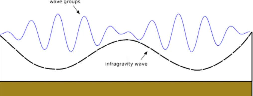
1.1 The Longuet-Higgins and Stewart theory of infragravity-wave formation. Wave group (blue line) and induced infragravity wave (black line). . . 2 1.2 Zone division of the nearshore region (from Coastal

Wiki). . . 3 1.3 The three main types of breaking waves. All

inter-mediate states may appear on a real beach. . . 6 1.4 Spilling Breakers. . . 7 1.5 Plunging breakers . . . 7 1.6 Surface profile of linear wave (top panel),

second-order Stokes correction profile (middle panel) and surface profile of a second-order Stokes wave (bottom panel; from Holthuijsen (2010)). . . 10 1.7 Surface profile of a cnoidal wave train (from

Holthui-jsen (2010)). . . 10 1.8 Illustration of the role of the SZ in generating/reflecting

LFW. Wave groups reflected at a wall (panels a and c). Wave groups generating a SZ (panels b and d). Characteristic curves and shoreline position in the (x, t)-plane (panels a and b). Normalized inci-dent (thin line) and reflected (thick line) Riemann variables at the offshore boundary (panels c and d). From Bellotti and Brocchini (2005). . . 20

(12)

2.1 The COAWST Modeling System that joins an Ocean model, an Atmosphere model, a Waves model, and a Sediment Transport Model for studies of coastal change . . . 31

2.2 Representation of a typical ROMS grid (from Wiki ROMS). . . 32

2.3 The split time stepping used in the model (Hedström 2016). . . 33

2.4 Flowchart of the embedded SBCs routine. . . 38

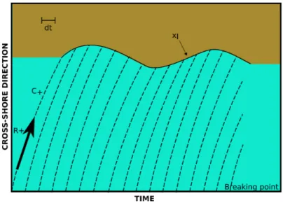
2.5 Illustration of the flow representation in the (space, time) -plane near to the shoreline. The incoming characteristic curve (C+) carries information on the

incident Riemann variable(R+) to the mean

shore-line (xl), here taken as the envelope of the run-down

positions. . . 39

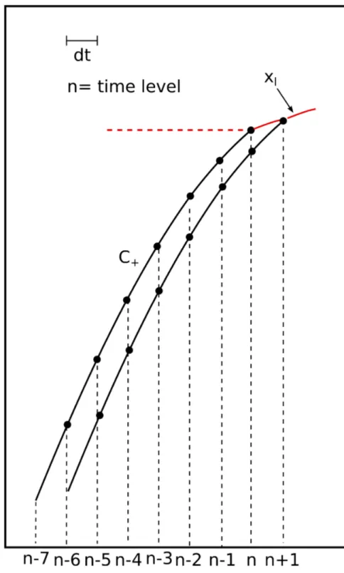
2.6 Illustration of the flow representation in the (space, time) -plane near to the shoreline. The incoming characteristic curve (C+) carries information on the

incident Riemann variable(R+) to the mean

shore-line (xl), here taken as the envelope of the run-down

positions. . . 40

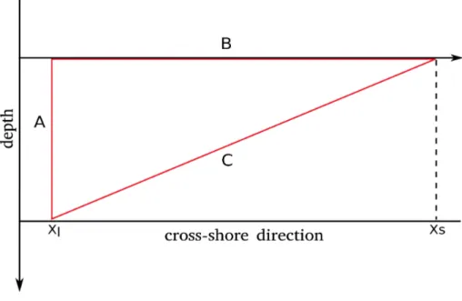
2.7 Wedge model used as simple approximation of the swash zone region. A = depth at xl, B = xs− xl . . 41

(13)

List of Figures 2.8 Sketch of few cross-shore sections of Arakawa-C grid

with xl (pentagon) falling in different wet-dry areas.

Circles represent rho-points while squares represent

u-points, with dotted lines indicating dry nodes and

solid lines indicating wet nodes: (a) xl completely

surrounded by wet points, (b) rho-points and u-point seaward of xl are wet while u-point landward of xl is

dry, (c) u-points and rho-point seaward of xl are wet

while the rho-point landward of xl is dry, (d)

rho-and u-points seaward of xl are wet while both

rho-and u-points lrho-andward of xlare dry, (e) xlcompletely

surrounded by dry points. . . 44

3.1 Bathymetry used for all the test cases. . . 46 3.2 Dimensionless results for Test case 1: evolution of

H0at the offshore boundary (top-left panel); mid

do-main cross-shore section at different times of: wave setup (top-right panel), H (bottom-left panel) and

ubar (bottom-right panel). . . . 48 3.3 Shoreline (dimensionless) evolution for the first 10

minutes of runs with a L0/170 cross-shore resolution.

The black line represents xl computed with ROMSrs,

while the red line gives xl computed with ROMSSBCs. 49

3.4 Evolution at xl of the right-hand side terms of

equa-tion (2.21a), in dimensionless form: first term (black line), second term (red line), and third term (green line). . . 50 3.5 Shoreline (dimensionless) evolution for the first 10

minutes of run (about 120 input periods) with a

L0/170 cross-shore resolution (green line) and

(14)

3.6 Dimensionless results for Test case 2: evolution of H0

at the offshore boundary (top-left panel); cross-shore section at different times of: wave setup (top-right panel), H left panel) and ubar (bottom-right panel). . . 52 3.7 Dimensionless results for test case 2: shoreline

evolu-tion for the first 10 minutes of run (about 5 Ttr) using

grids with different cross-shore resolution. The black lines represents xlcomputed with ROMSsl, while the

red lines give xl computed with ROMSSBCs. . . 53

3.8 Dimensionless results for test case 2: shoreline evolu-tion for the last 10 minutes of run (about 5 Ttr) using

grids with different cross-shore resolution. The black lines represent xl computed with ROMSsl, while the

3.9 Dimensionless results for test case 2: shoreline evolu-tion for the last 10 minutes of run (about 5 Ttr) using

grids with different cross-shore resolution. The black lines represent xl computed with ROMSrs, while the

3.10 Dimensionless results for Test case 3: evolution of H0

at the offshore boundary (top-left panel); cross-shore section at different times of: wave setup (top-right panel), H left panel) and ubar (bottom-right panel). . . 56 3.11 Dimensionless results for Test case 3: shoreline

evo-lution for the first 10 minutes of run (about 5 Ttr)

using grids with different cross-shore resolution. The black lines represents xlcomputed with ROMSsl, while

(15)

List of Figures 3.12 Dimensionless results for Test case 3: shoreline

evo-lution for the last 10 minutes of run (about 5 Ttr)

using grids with different cross-shore resolution. The black lines represent xlcomputed with ROMSsl, while

the red lines give xl computed with ROMSSBCs. . . 59

3.13 Dimensionless results for Test case 3: shoreline evo-lution for the last 10 minutes of run (about 5 Ttr)

using grids with different cross-shore resolution. The black lines represent xlcomputed with ROMSrs, while

the red lines give xl computed with ROMSSBCs. . . 60

3.14 Dimensionless results for Test case 3: shoreline evo-lution for the last 10 minutes of run (about 5 Ttr;

green line) and characteristic curves below it (equa-tion 2.24; black lines). . . 61 3.15 Dimensionless results for Test case 3: evolution at

xl of the right-hand side terms of equation (2.21a):

first term (black line), second term (green line), and third term (red line). . . 62 3.16 Results for Test case 3: near shoreline depth.

Solu-tion obtained with (from the top to the bottom): ROMSrs, ROMSSBCs with L0/12, ROMSSBCs with L0/3 and ROMSSBCs with L0/2. . . . 63

3.17 Results for Test case 3: near shoreline cross-shore velocity. Solution obtained with (from the top to the bottom): ROMSrs, ROMSSBCswith L0/12, ROMSSBCs

with L0/3 and ROMSSBCs with L0/2. . . . 64

3.18 Sensitivity analysis for the function Cv. The black line represents xldimensionless computed with ROMSrs,

while the other lines represent the dimensionless shore-lines obtained with ROMSSBCs using different values

for Cv. Red line: Cv = 0.615 − 0.201f , blue line:

Cv = 0.400 − 0.201f , green line: Cv = 0.800 − 201f ,

cyan line: Cv = 0.615 − 0.101f , grey line: Cv = 0.615 − 0.301f . . . . 65

(16)

3.19 Dimensionless shoreline evolution for the last 10 min-utes of run (about 5 Ttr). The black line is xl

ob-tained with ROMSrs, the red line is xlobtained with

ROMSSBCs and the green line is xl obtained with

ROMSSBCsexcluding the third term of equation (2.21a). 66

3.20 Dimensionless results of the sensitivity analysis on the starting point for the propagation of R+.

Shore-line evolution for the last 10 minutes of run (about 5 Ttr) using different starting points for the

propa-gation of R+. The black lines represent xl computed

withROMSrl, while the red lines give xl computed

withROMSSBCs. . . 68

3.21 Dimensionless results of the sensitivity analysis on the starting point for the propagation of R+.

Shore-line evolution for the last 10 minutes of run (about 5 Ttr; green line) and incoming characteristic curves

(equation 2.24; black lines). . . 69 3.22 Dimensionless results of the sensitivity analysis on

the starting point for the propagation of R+.

Evo-lution at xl of the right-hand side terms of equation

(2.21a): first term (black line), second term (green line), and third term (red line). . . 70 3.23 Fourier analysis results. xlfrom ROMSrs(top panel)

and its Fourier transform (bottom panel). . . 71 3.24 Fourier analysis results. xl from ROMSSBCs with a

cross-shore resolution of L0/120 (top panel) and its

Fourier transform (bottom panel). . . 71 3.25 Fourier analysis results. xl from ROMSSBCs with a

cross-shore resolution of L0/12 (top panel) and its

Fourier transform (bottom panel). . . 72 3.26 Fourier analysis results. xl from ROMSSBCs with

a cross-shore resolution of L0/3 (top panel) and its

(17)

List of Figures 3.27 Fourier analysis results. xl from ROMSSBCs with

a cross-shore resolution of L0/2 (top panel) and its

Fourier transform (bottom panel). . . 73 3.28 Fourier analysis results. The three terms of the right

hand side of equation (2.21a) from ROMSSBCs with

a cross-shore resolution of L0/2. First term (top

panel), second term (middle panel) and third term (bottom panel). . . 73 4.1 Mid domain cross-shore section at different times of

the phase speed c (resolution of about L0/120 ; wave

(18)

(19)

List of Tables

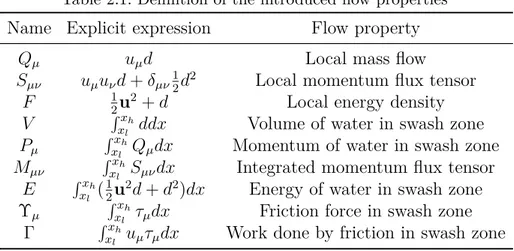
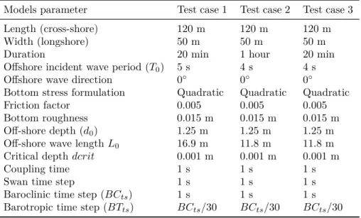
2.1 Definition of the introduced flow properties . . . 24 3.1 Model parameters for the three test cases . . . 47

(20)

(21)

Chapter 1 Introduction

The interest of scientists, coastal engineers and stakeholders in coastal environments has grown over the last 20 years with specific reference to various issues (coastal erosion, bathing water quality, runoff from rivers and dumping etc.).

The waves we normally observe when standing in front of the ocean are generated by the momentum transfer from the wind to the sea surface (Miles 1957; Phillips 1957). As waves propagate across the ocean, this energy is carried with them. When waves enter wa-ter with depth approximately half of their wavelength, they start to be affected by the sea bed. Moving shoreward waves find progres-sively shallow water where energy begins to dissipate through bed friction and turbulent breaking till the swash zone. Here the energy left is both dissipated or reflected back offshore. These waves are normally referred to as short waves or incident waves. This class of waves can be further subdivided into wind waves (locally generated and with frequency of few Hz and swell (generated far from the site of interest and with frequency of about 0.1Hz)

Another very important forcing for the nearshore flows are low-frequency waves. The existence of long-period ocean waves (also called infragravity waves) has been acknowledged for some time (Munk 1949 and Tucker 1950). The amplitude of these waves was shown to have a quasi-linear relationship with the amplitude of the incident waves at the seaward limit of the surf-zone (Tucker 1950). Infragravity waves are difficult to measure and scientists

(22)

are still partly relying on theoretical approaches to describe them. One of these theories comes from the work of Longuet-Higgins and Stewart (1964), in terms of radiation stress. Since large waves have a greater radiation stress than small waves, then this difference in momentum flux causes water to be expelled from regions of larger waves to regions of smaller waves, within the group. This causes a "set down wave" which is 180◦ out of phase with the envelope of the wave-group, but has the same wavelength and period (see figure 1.1 for an illustration of this concept).

Figure 1.1: The Longuet-Higgins and Stewart theory of infragravity-wave formation. Wave group (blue line) and induced in-fragravity wave (black line).

An alternative theory to explain the formation of low frequency oscillations in the surf-zone was proposed by Symonds, Huntley, and Bowen (1982). Here the generation of long waves oscillation is explained as time-varying wave set-up. This because of a cross-shore variation in the position of the breakpoint due to the variation in the hight of the incident waves.

1.1 The nearshore zone

The nearshore coastal region can be defined as the region between a fictive offshore limit, which usually is considered as the limit where the depth starts to influence the waves and the shoreline. The wave

(23)

1.2 Short wave outside the surf zone motion itself determines this depth and in simple terms it can be identified as a depth of approximately half the wave lengh. With this definition in storms with larger and longer waves the offshore limit moves further out to sea.

The nearshore zone can be schematically divided into a number of regions: the wave shoaling zone, the outer surf zone, the inner surf zone and the swash zone (see figure 1.2). The wave shoaling zone is the most offshore region. Here unbroken waves start to interact with the sea bed. In the outer surf zone waves begin to break and rapid transformation in wave shape occurs. The inner surf zone is typically characterised by the majority of waves being broken and rather slow changes in wave shape. Landward of the inner surf zone and linking the wet and dry parts of the beach, is the swash zone where waves run up and back across the beachface.

Figure 1.2: Zone division of the nearshore region (from Coastal Wiki).

1.2 Short wave outside the surf zone

In deep water the short wave profile is approximately sinusoidal in both space and time (sea figure 1.6) and is well described by the linear wave theory (Airy 1841). In the linear wave theory, the water

(24)

surface (η ) is given by:

η (x, t) = a cos(kx − ωt) (1.1)

where x is the coordinate pointing in the direction of wave prop-agation, t is the time, k = 2π

L is the wavenumber, ω = 2π

T is the

angular frequency, T is the wave period, a is the wave amplitude and L is the wavelength. The wavelength is then given by:

L = gT 2 π tanh (_2πd L ) (1.2) where g is the acceleration due to gravity and d is the water depth. The wave speed c can be calculated using:

c = L

T (1.3)

As waves move shoreward into progressively shallower water, the wave speed decreases because the wavelength decreases. The de-creases in wave length causes an increase in wave energy density due to an increase in wave height. Furthermore, the nearly sinu-soidal profile that waves have is lost and waves becomes increasingly non-linear, with narrow peaked crests and wide flat troughs. The transition from linearity to non-linearity through shoaling can be represented by the Ursell parameter (Ursell 1953):

Ur =

HL2

d3 (1.4)

with H representing the wave height. It is important to acknowl-edge that despite wave shoaling is most pronounced outside the surf zone, it also occurs inside the surf zone.

(25)

1.3 The Surf zone

1.3.1 Short wave breaking

A stable waveform is not possible when waves are in too shallow water, thus they break. Breaking occurs because waves become too steep, with too much energy concentrated in their front and water particles in the wave crest traveling with velocities higher than C. A "saturation type" breaking criterion gives:

Hbr = γbrdbr (1.5)

where the subscript br indicates breaking conditions and γbr is the

breaker index, which relates the height of the breaking wave with the local water depth.

This breaking criterion and the value of γbr was the subject of

several studies. Battjes and Janssen (1978) re-analysed data of a number of laboratory and field experiments for various types of bottom topography and found values of γbr ranging between 0.6

and 0.83. Later Kaminsky and Kraus (1993) found, using data obtained in a large number of experiments, values in the range 0.6-1.59. Clearly, γbr cannot be thought of being an universal constant

and its value seems to depend on both bottom slope and incident wave steepness. For instance, Battjes and Janssen (1978) suggest:

γbr =

Hbr

dbr

= 0.5 + 0.4 tanh(33so) (1.6)

s0 = H0_L0 being the offshore wave steepness, with H0 the offshore

wave height and L0 the offshore wavelength. It is important to

remark, that most saturation breaking conditions and indices come from laboratory experiments where purely monochromatic waves have been used.

Breaking can be classed into three types of conditions: spilling, plunging and surging breakers (see figure 1.3). Spilling breakers (figure 1.4) are associated with gently sloping beaches and steep

(26)

incident waves. They are characterised by gentle spilling of foam from the crest.

STEEP BEACH

SURGING BREAKER MODERATE SLOPING BEACH

PLUNGING BREAKER GENTLY SLOPING BEACH

SPILLING BREAKER

Figure 1.3: The three main types of breaking waves. All intermediate states may appear on a real beach.

Plunging breakers (figure 1.5) are associated with intermediate beach slopes and waves of intermediate steepness. In this case, the wave face becomes vertical and the crest of the wave curls over

(27)

1.3 The Surf zone and plunges forward and downwards. Both spilling and plunging breakers are observed in the surf zone.

Figure 1.4: Spilling Breakers.

Figure 1.5: Plunging breakers

Surging breakers occur on steep beaches with incident waves of low steepness. In surging breaker, the waves move up the beach without breaking, resulting in a large proportion of energy reflected offshore. Surging breakers are generally restricted to the swash zone.

A fourth breaking wave type was also identified by Galvin (1968): a collapsing breaker. This breaker type is intermediate between the plunging and surging breaker types.

(28)

1.3.2 Short waves within the surf zone

Energy inside the surf zone can be saturated or unsaturated. In a saturated surf zones, the wave height is dependent on local (depth) parameters and independent by the offshore wave height (Goda 1975, Wright and Short 1984, Raubenheimer and Guza 1996).

Wave characteristics keep changing as waves move through the surf zone. The current conceptual model of the surf zone divides the surf zone into outer and an inner region (Svendsen, Madsen, and Hansen 1978). The outer surf zone is where the largest waves break and where there are rapid transitions in wave shape. In the inner surf zone, most of the waves are broken and the rate of change in the wave shape is relatively slow, the waves having a quasi-steady (saw-tooth type) form throughout this region. Waves in this region are very similar to a moving bore. This region extends to the swash zone. These different regions can be parameterised in terms of the Ursell number Ur, which assumes higher values moving toward the

shoreline.

The most common way to describe waves is by their (H) and (T ). However, once waves enter the surf zone, they become increasingly non-linear and this parameter does not capture this change (sea figure 1.6 bottom panel). One useful parameter to capture these shape changes was described by Cowell (1982). This parameter is calculated using ln (e/b, where e is the time from the minima of the preceding trough to the crest of the wave and b is the time from the crest of the wave to the subsequent trough minima.

When waves are too steep or water is too shallow, the linear wave theory is no longer valid and the waves are described through a nonlinear theory. In classical non-linear theories, flow properties are expressed as the sum of functions, dependent on the power of a perturbative parameter. Here we briefly introduce two of the classical nonlinear theories: the theory of Stokes (1847) for steep waves and the cnoidal theory for waves in shallow water (Korteweg and De Vries 1895). In the Stokes theory the basic harmonic is

(29)

1.3 The Surf zone corrected (second-order correction) with an ‘extra’ harmonic wave, written with the perturbative parameter ϵ = ak raised to the second power:

η(x, t) = ϵη1(x, t) + ϵ2η2(x, t) (1.7)

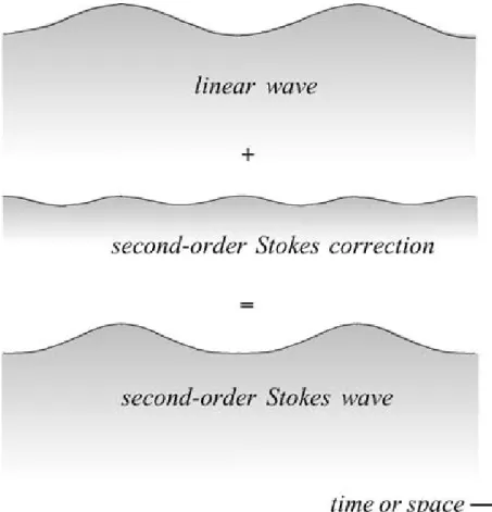
where the first term on the right-hand side is the Airy wave of the linear wave theory (figure 1.6 top panel) and the second term is the second-order Stokes correction (figure 1.6 middle panel). The wave represented by equation (1.7) is called a second-order Stokes wave. If depth is small the Stokes theory is no longer valid. Therefore, in addiction to, or instead of, considering nonlinear corrections due to wave steepness, corrections need to be applied to account for finite-depth effects. This is done in the theory of cnoidal waves in a fashion similar to that of Stokes theory. Here the perturbative parameter β is equal to a/d. Stopping at the second-order the surface elevation is, then, written as

η(x, t) = βη1(x, t) + β2η2(x, t) (1.8)

where, the basic wave η1 and the extra wave η2 are not harmonic

waves but cnoidal waves (see figure 1.7).

1.3.3 Surf zone saturation

A large range of scales and types of fluid motion may be present in the inner surf zone, which will subsequently govern the shoreline oscillation and swash hydrodynamics. These include short (high-frequency) waves, long waves, edge waves, shear waves, cross-shore and longshore currents, turbulence and vortices.

Energy inside the surf zone can be saturated or unsaturated. In a saturated surf zone, the wave height is dependent on local (depth) parameters and independent of offshore wave height (sea equations 1.5 and 1.6). In contrast, unsaturated surf is defined by conditions where an increase in offshore wave height leads to an increase in surf zone wave height (Goda 1975, Wright and Short

(30)

Figure 1.6: Surface profile of linear wave (top panel), second-order Stokes correction profile (middle panel) and surface profile of a second-order Stokes wave (bottom panel; from Holthuijsen (2010)).

Figure 1.7: Surface profile of a cnoidal wave train (from Holthuijsen (2010)).

(31)

1.3 The Surf zone 1984, Raubenheimer and Guza 1996). In the first case, typical of gently sloping beaches, the inner surf zone hydrodynamics may be expected to be dominated by non-breaking low-frequency waves (Huntley, Guza, and Bowen 1977, Guza and Thornton 1982, Goda 1975, Wright, Guza, and Short 1982). In unsaturated surf zones low frequency waves may still dominate the shoreline motion (Brocchini and Baldock 2008), but in addition to standing low-frequency waves a significant contribution exists from frequency down shifting (Mase 1995), wave grouping remaining in the unsaturated inner surf zone and swash-swash interactions (Baldock, Holmes, and Horn 1997).

1.3.4 Long waves

Field studies on gently sloping beaches have indicated that while the short wave energy is dissipated due to wave breaking, infra-gravity energy increases across the surf zone as depth decreases and it is carried through to the shoreline (Guza and Thornton 1982). Therefore, in incident-saturated conditions, the shoreline becomes increasingly long-wave dominated with increasing offshore wave height (Butt and Russell 2000)

Short waves, due to their short wavelength generally break before they reach the shoreline with subsequent energy loss. In contrast, infragravity oscillations, having a larger wavelength never become steep enough to break. However, infragravity waves do start to interact with the bottom and slow down.

The wave front slows down before the wave tail, causing an in-crease in amplitude with a subsequent inin-crease in energy. Because of their low frequency, long-waves are typically reflected from the shoreline. They may either remain trapped to the shore as an edge wave (Huntley 1976), or leak out into deeper water.

Further, the interaction between the shoreward-propagating wave and its reflection from the beach face may lead to the production of a standing wave. Long waves alter the mean water depth in the surf zone on time scales ranging from 20 seconds to several

(32)

minutes. This changes the local water depth that the incident waves propagate into, this altering the propagation of the short waves.

1.4 The swash zone

The collapse of the flow on to a moving shoreline leads to flow depths at the runup tip (Shen and Meyer 1963) and throughout the swash zone that are very small when compared with the length scale of the horizontal flow. In these conditions the flow is prac-tically tangential to the beach, which allows for use of the Non-linear Shallow Water Equations (NSWEs) as the preferential tool to study this part of the foreshore with good confidence (Peregrine 1972, Brocchini and Baldock 2008).

Although the swash zone moves over the whole of the intertidal zone, the local swash zone may be defined as the region of the fore-shore where the wave action (uprushes and backswashes) moves the instantaneous shoreline back and forth around the mean water level (Holman 1986, Elfrink and Baldock 2002). The moving shoreline makes this area to be alternatively exposed to the atmosphere or covered by water thus, flow properties here are only defined for short intervals (Brocchini and Baldock 2008).

The swash zone is arguably the most complex area of the coast-line. It can be seen as a highly dynamic and changeable boundary layer between land and sea, where many hydrodynamics and mor-phological events occur over a wide range of time scales. Swash motions are characterized by a great turbulence level, highly un-steady flows, considerable sediment transport and rapid morpho-logical changes (Brocchini 1997, Puleo et al. 2000, Masselink and Puleo 2006, Brocchini and Baldock 2008).

This region is well defined for monochromatic waves while this is not true for real sea states where runup and rundown and setup vary constantly with time. In this context, the swash zone may be de-fined as the region in which the beach face is intermittently exposed to the atmosphere, possibly over both long (minutes) and short

(33)

(sec-1.4 The swash zone onds) time scales (Elfrink and Baldock 2002). Two broadly different types of swash oscillations have been identified by theoretical, field and laboratory studies, consistent with the forcing at the seaward swash boundary (see section 1.3.3). Typically swash motions may result from non-breaking standing waves or broken short waves.

1.4.1 Swash zone hydrodynamics

Swash zone boundary conditions

The swash zone hydrodynamics is mainly forced by boundary condi-tions imposed by the inner surf zone and beachface features. Along this boundary the forcings include wave or bore height, period, waveshape, orbital velocities, currents, turbulence, beach slope and beach composition (Elfrink and Baldock 2002). From the above it is clear that, in order to properly predict the swash zone hydrody-namics, it is crucial to have a thorough understanding of the inner surf zone processes (see 1.3.3).

Swash oscillations

The swash motion features change depending on the beach con-figuration, hydraulic forcing and gradient and mean sediment size. Thus, an unambiguous definition of swash characteristics is not re-ally possible.

One classification based on beach topography divides into swash zones typical of dissipative beaches and reflective beaches. Dissipa-tive beaches are generally typified by a gently sloping bathymetry and relatively fine sediments. In this condition the surf zone is nor-mally saturated and the swash motion is imposed by low frequency oscillations, being the short wind wave energy dissipated through a wide surf zone. In contrast, reflective beaches feature steeper gradients where most of the wave energy is reflected offshore and the only swash is due to bores collapsing at the shoreline. Here the dominant swash motion is defined by the incoming short wave

(34)

approaching the beach face as breaking bores. In parallel with this considerations typical swash periods may range from seconds on steep, reflective beaches, to minutes on gentle, dissipative beaches (Hughes, Masselink, and Brander 1997, Butt and Russell 1999). Generally, in both cases the swash zone works as a dissipation area for high frequency waves, while long waves are reflected seaward (Brocchini and Baldock 2008)

It is obvious that the only-dissipative or the only-reflective case are just a theoretical matter. On natural beaches real swashes are always driven by both short and long waves.

The high complexity of the swash zone dynamics suggests to neglect bottom friction and flow infiltration/exfiltration across the bed boundary to give a first description of it. With this simplified approach a single runup event consequent to an incident broken wave (surf zone bore) propagating perpendicular to the coast can be described as follows:

1. At the breakpoint the wave starts to dissipate energy because of breaking-induced turbulence, with a consequent H decrease.

2. In the surf zone the wave height decreases approximately as a linear function of the water depth.

3. Approaching the local instantaneous shoreline (zero depth), the bore front and the water behind the bore front abruptly accel-erate (Whitham 1958, Brocchini and Baldock 2008) and the bore collapses (swash uprush) (Shen and Meyer 1963, Brocchini and Bal-dock 2008) with its potential energy being suddenly transformed into the kinetic energy of a thin wedge of water whose tip propa-gates up the beach face.

4. Once the swash has reached its maximum uprush, the flow reverses and accelerates offshore forming the backswash. As for the uprush, the swash surface is seaward dipping for the whole of the backwash phase. It is important to note that the flow reversal does not occur simultaneously at all cross-shore locations (Hibberd and Peregrine 1979). In general, the uprush is of shorter duration compared to the backwash but has flow velocities of greater absolute

(35)

1.5 Nearshore circulation models magnitude (Hughes, Masselink, and Brander 1997).

Swash-swash interaction

When a sequence of waves approaches the beach, the intensity of the swash-swash interaction within the surf zone can be described by the ratio between the period Ts of a individual swash event and

the incident wave period T . If T > Ts normally there is little or

no interaction, while the case of Ts ≥ T corresponds to strong

interaction.

Swash-swash interactions occur when there is interaction between incident waves and the runup or backwash of the preceding waves. These interactions generate a broad range of scales and new motions comprising: low-frequency waves, backwash bores and hydraulic jumps, and turbulence (Brocchini and Baldock 2008).

The interaction between high-frequency swash and standing long waves in the swash zone is also a very important feature for both the hydrodynamics and the beach face morphology. The long waves act likewise a tide, moving the short-wave swash across the beach face increasing the active swash zone width (Brocchini and Baldock 2008).

Short-wave runup may coincide with the standing wave runup increasing swash amplitudes through constructive interference. De-structive interference occurs if runup and backwashes oppose each other (Brocchini and Baldock 2008).

1.5 Nearshore circulation models

In the last 40 years Boussinesq-type models (BTMs) became the most used tools for coastal-type computations. The reason for this success is their ability to represent all main physical phenomena and their numerical cheapness (Brocchini 2013). Boussinesq (1872), was the first to tackle the problem of solving the Navier Stokes equations in shallow waters. With the increase of computation power,

(36)

com-puters became available for scientific-purpose calculations. Thus, it was possible to couple the power of mathematical and numeri-cal techniques and, hence, the pioneering contribution by Peregrine (1967).

Two classes of BTMs rise, distinguishing between: BTMs with the assumption of irrotational flow and BTMs which compute ro-tational flow. In the former class, vorticity injection at the bottom and free-surface boundary layers are taken as negligible. For this kind of BTMs, breaking dissipation and parametrized bottom fric-tion need to be externally added (Brocchini 2013). The external breaking-induced dissipation can be based on the ‘surface roller’ concept (Svendsen 1984). Different is the situation for the lat-ter class where, dissipative mechanisms induced by wave breaking, rather than being externally added, naturally stem from the equa-tion derivaequa-tion procedure (Veeramony and Svendsen 2000). This class of BTMs seems to be more suited to reproduce surf zone flows. However, they require closures for both vorticity and tur-bulence (Brocchini 2013). The class of ‘rotational flow’ BTMs even though used for scientific studies, are practically no used at the op-erational level. The reasons for such a partial success are several, among the most important: the difficulty in physically describing the required closures and numerically implementing them into an efficient code (Brocchini 2013).

The temporal evolution of Boussinesq-type models has been mainly pushed by practical requirements. In particular, the coastal engi-neering community has been largely involved in the process of ex-tending the region of validity of BTMs towards the intermediate-to-deep waters, on one hand, and towards the near-shoreline dynamics on the other hand.

In early BTMs, the effects of nonlinearity were treated as a weak perturbation to a primarily linear problem. However, in many practical cases (i.e. shoaling waves and breaking waves), nonlin-ear effects are too strong and this kind of approach is not efficient anymore and a fully nonlinear approach is necessary. This was the

(37)

1.5 Nearshore circulation models focus of research in BTMs over the first decade of the 2000s (Mad-sen, Bingham, and Schäffer 2003, Mad(Mad-sen, Fuhrman, and Wang 2006, Bingham, Madsen, and Fuhrman 2009).

Computations of coastal flows is normally carried out either at a wave-resolving or at a wave-averaged level. However, when at-tempting very long simulations over spatial areas of the order of 10Km2 _{or larger the limits of wave-resolving models come out.}

When this kind of computations is needed the best solution is to resort to wave-averaged models.

Averaging shallow-water-type equations over the period of short waves leads to wave-averaged two-dimensional horizontal (2DH) models, where the closure problem is that of representing the unre-solved short-wave motion. These contributions appear in the mo-mentum equation as radiation stresses. Ever since the concept of ra-diation stress was presented by Longuet-Higgins and Stewart (1964) nearshore simulations have been carried out by wave-averaged mod-els.

The first of these wave-averaged models were relatively simple theoretical solutions of longshore currents driven by radiation stress gradients (Longuet-Higgins 1970). One of the first numerical mod-els for nearshore circulation was developed by Noda (1974). The model was used to study steady flows with longshore varying topog-raphy and to model circulation patterns with rip currents. Other important early nearshore circulation models were those by Eber-sole and Dalrymple (1980) and Wu and Liu (1985). These models were all 2DH models, which, essentially solve the shallow water equations.

1.5.1 Quasi-3D circulation models

The development of quasi-3D models began with De Vriend and Stive (1987) who divided the currents into primary and secondary components. The primary current was forced by the depth-invariant terms (i.e. the pressure gradient) while the secondary current was

(38)

driven by the depth-varying forcing. Alternatively, Svendsen and Lorenz (1989) assumed the cross-shore and longshore currents were weakly dependent on each other, this resulting in a current pro-file with a spiral shape. Svendsen and Putrevu (1990) solved the vertical profiles and used the result in a depth-averaged numeri-cal model. Svendsen and Putrevu (1994) found that the current-current and wave-current-current interaction terms were inducing non-linear mixing many times stronger than the turbulent mixing from wave breaking. A generalized version of these mixing terms was derived by Putrevu and Svendsen (1999). A simplified version of the 3D dispersive mixing is included in the nearshore circulation model SHORECIRC, as described by Svendsen, Haas, and Zhao (2002) and Haas, Svendsen, et al. (2003).

The primary advantage of quasi-3D models is that they solve for the vertical variation of the currents and included the leading-order effect of the depth-varying currents on the depth-averaged flow field all on a two-dimensional grid, preserving the computational speed of a 2DH model.

1.5.2 Fully 3D circulation models

In the last years several effort even been put to introduce the effects of waves on ocean currents using fully three dimensional numerical models. Some of the most successful works were carried out with the Regional Ocean Modeling System (ROMS) Haas, Svendsen, et al. (2003), Haidvogel et al. (2008), Shchepetkin and McWilliams (2005), and Uchiyama, McWilliams, and Shchepetkin (2010). See section 2.2.1 for a detailed description of ROMS.

1.5.3 SHORECIRC Vs ROMS

Haas and Warner (2009) compared the quasi-3D SHORECIRC cir-culation model to the fully 3D ROMS circir-culation model for test case called "Shoreface". In the following we recall the main conclusions of their work.

(39)

1.5 Nearshore circulation models The two models’ performances are compared for three wave con-ditions: 1) spectral waves approaching a plane beach with an oblique angle of incidence; 2) monochromatic waves driving longshore cur-rents in a laboratory basin; and 3) monochromatic waves on a barred beach with rip channels in a laboratory basin.

For tests 1 and 2, depth-averaged quantities are nearly identical for the two models and similar results for the same quantities for the two models are also found for test case 3. The small differences observed in the latter test are due to either different boundary conditions or different turbulence closures used in the two models. The differences in the vertical variation of the currents between the two models are primarily a result of the method for incorporating the vertical variation of the radiation stresses.

Being ROMS a 3D model, the radiation stresses parameterization allows for vertical variability. On the other hand, in SHORECIRC, in order to simplify the integration of the depth varying currents, the long wave theory for a sloping bottom is used for the formulation of the radiation stress terms in the momentum equations that retain vertical flow variability. However, in the depth-averaged equations of SHORECIRC, the radiation stress terms are calculated with the linear theory of waves evolving over a horizontal seabed. This cre-ates an inconsistency between the two radiation stress forcing. For both models, there is a local imbalance over the depth between the terms that are balanced in the depth-integrated momentum equa-tions. For ROMS this is mainly due to the vertical variation of the radiation stress whereas, for SHORECIRC it is a consequence of the above mentioned over-simplified calculation of the radiations stresses. This imbalance is generally compensated by the vertical viscosity term, resulting in differing vertical variation of the cur-rents for the two models.

The quasi-3D model is computationally faster when run on a single processor. However ROMS is designed to use either OpenMP (shared memory) or MPI (distributed memory) systems, thus, the overall computational speed of ROMS can be faster. Further, the

(40)

fully 3D model can be applied to include more processes like river flows, tracer advection, stratification, Coriolis forcing, and can span across a broader range of spatial applicability.

1.5.4 The shoreline of wave-averaged models

The use of these models allowed a good representation of the phe-nomena evolving in the nearshore area, especially when coupled to wave drivers to represent the effects of waves on ocean cur-rents. Although well developed, wave-averaged models use some assumptions that limit their capability of reproducing natural flow conditions. One of the most crucial shortcomings concerns the rep-resentation of the swash zone dynamics. Typical circulation models use simplified boundary conditions such that perfect absorption or perfect reflection (rigid wall) is enforced at the inshore boundary of the computational domain.

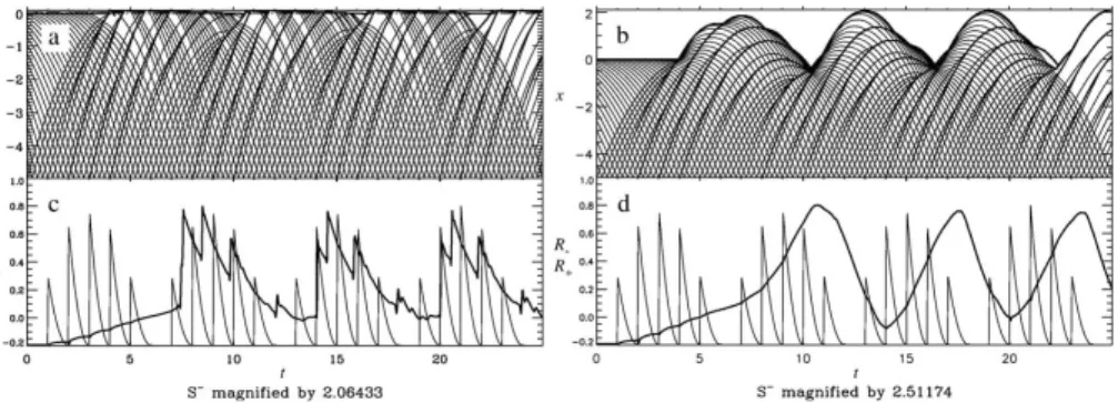
However, within the infinitesimal swash zone prescribed through a wall condition no generation or modification of low-frequency waves can occur and all incoming low frequency waves are reflected at a single point (Brocchini and Baldock 2008).

Figure 1.8: Illustration of the role of the SZ in generating/reflecting LFW. Wave groups reflected at a wall (panels a and c). Wave groups generating a SZ (panels b and d). Characteris-tic curves and shoreline position in the (x, t)-plane (panels a and b). Normalized incident (thin line) and reflected (thick line) Riemann variables at the offshore boundary (panels c and d). From Bellotti and Brocchini (2005).

(41)

1.5 Nearshore circulation models The present thesis work explores the possibility of implementing into available wave-averaged solvers, a theoretical model (Brocchini and Peregrine 1996, Brocchini and Bellotti 2002, Antuono, Broc-chini, and Grosso 2007) that gives full account, through an integral approach, of the swash zone dynamics. Once such model is im-plemented, the wave-averaged solver will be able to calculate the position of a mean shoreline and provide along it shoreline boundary condition (SBCs) that take in account of the swash zone dynamics (see section 2.3 for the description of the theoretical model).

(42)

(43)

Chapter 2 Methods

2.1 The integral SBCs model

A detailed description of the integral model SBCs by Brocchini & Coauthors is given in the following. Suitable boundary conditions are defined for wave-averaged models that fully take account of the swash zone dynamics. All the contents and materials used in this section come from Brocchini and Peregrine (1996) and Brocchini and Bellotti (2002). The new boundary condition are based on the NLSWE. These equation are depth integrated and obtained by as-suming that vertical accelerations of water, or those normal to the beach, are negligible compared with gravity. The general set of di-mensionless NLSWE (no specific notation is used for didi-mensionless variables) put in conservation form and completed with the energy equation and a dimensionless bed friction ⃗τ = (τ1, τ2) is:

dt+ (ud)x+ (vd)y = 0, (2.1a) (ud)t+ (u2d + 1 2d 2₎ x+ (uvd)y + d + τ1 = 0, (2.1b) (vd)t+ (uvd)x+ (v2d + 1 2d 2₎ y + τ2 = 0, (2.1c) 1 2[d(u 2_{+ v}2_{) + d}2_] t+ ( 1 2u 3_{d +} 1 2v 2_{ud + ud}2₎ x+ (1 2v 3 d + 1 2u 2 vd + vd2)y + u(d + τ1) + vτ2 = 0, (2.1d)

(44)

Table 2.1: Definition of the introduced flow properties Name Explicit expression Flow property

Qµ uµd Local mass flow

Sµν uµuνd + δµν1₂d2 Local momentum flux tensor

F 1₂u2_{+ d} _{Local energy density}

V ∫xh

xl ddx Volume of water in swash zone

Pµ ∫xxlhQµdx Momentum of water in swash zone

Mµν

∫x_h

xl Sµνdx Integrated momentum flux tensor

E ∫xh

xl (

1

2u

2_{d + d}2_)dx _{Energy of water in swash zone}

Υµ

∫xh

xl τµdx Friction force in swash zone

Γ ∫xh

xl uµτµdx Work done by friction in swash zone

where u and v are, respectively, the cross-shore component and the long-shore component of the flow velocity. The swash zone limits are xl, the seaward (lower) and xh shoreward (higher) limits. The

seaward boundary may be chosen to be the lowest limit xl, of the

moving shoreline in a group of waves. Integration of equations (2.1) over the swash zone width for constant xl gives:

∂V ∂t = ∫ xh xl dtdx = Q1(t)|xl− ∂P2 ∂y , (2.2a) ∂P1 ∂t = ∫ xh xl (ud)tdx = S11(t)|xl− V (t) − ∂M12 ∂y − Υ1(t), (2.2b) ∂P2 ∂t = ∫ xh xl (vd)tdx = S12(t)|xl− V (t) − ∂M22 ∂y − Υ2(t), (2.2c) ∂E ∂t = ∫ xh xl [1 2(u 2_{+ v}2_{)d + d}2_] tdx = F (t)Q1(t)|xl− P1(t) − ∂ ∂y ∫ xh xl F Q2dx − Γt, (2.2d)

These equations introduce flow properties integrated over the swash zone which are listed in table 2.1 where ⃗u = (u1, u2). The integral

flow properties, then, are used to seek appropriate boundary con-ditions at the seaward swash zone limit for wave-averaged models. This requires the knowledge of both long-wave motions and

(45)

short-2.1 The integral SBCs model wave motions contributes at the boundary xl.

To obtain dynamic equations suitable for wave-averaged model the basic flow properties u, v and d are splitted using a Reynolds-type decomposition into long-period and short-period properties:

u = ⟨u⟩ + ˜u, v = ⟨v⟩ + ˜v, d = ⟨d⟩ + ˜d, ⟨˜u⟩ = ⟨˜v⟩ =⟨d˜⟩= 0. (2.3) Here ⟨u⟩, ⟨v⟩ and ⟨d⟩ come from all motions whose typical time scale is significantly longer than the typical short-wave period. Whereas ˜u, ˜v and ˜d contributes are due to short-wave motions. By

substituting in the shallow water equations (2.1) for each flow vari-able and by phase averaging, a set of equations for long-period flow properties is obtained: ∂ ⟨d⟩ ∂t + ∂ ∂x [ ⟨u⟩ ⟨d⟩ +⟨Q˜1 ⟩] + ∂ ∂y [ ⟨v⟩ ⟨d⟩ +⟨Q˜2 ⟩] = 0 (2.4a) ∂ ∂t [ ⟨u⟩ ⟨d⟩ +⟨Q˜1 ⟩] + ∂ ∂x [ ⟨d⟩(⟨u⟩2+ ⟨˜u⟩2+ 1 2⟨d⟩ ) + 2 ⟨u⟩⟨Q˜1 ⟩ +⟨S˜11 ⟩] + ∂ ∂y [ ⟨d⟩(⟨u⟩ ⟨v⟩+ ⟨˜u˜v⟩)+ ⟨u⟩ ⟨Q2⟩ + ⟨v⟩ ⟨Q1⟩ + ⟨ ˜ S12 ⟩] + ⟨d⟩ = 0 (2.4b) ∂ ∂t [ ⟨v⟩ ⟨d⟩ +⟨Q˜2 ⟩] + ∂ ∂y [ ⟨d⟩(⟨v⟩2+ ⟨˜v⟩2+1 2⟨d⟩ ) + 2 ⟨v⟩⟨Q˜2 ⟩ +⟨S˜22 ⟩] + ∂ ∂x [

⟨d⟩(⟨u⟩ ⟨v⟩ + ⟨˜u˜v⟩)+ ⟨v⟩ ⟨Q1⟩ + ⟨u⟩ ⟨Q2⟩ +

⟨ ˜ S12 ⟩] = 0 (2.4c) The same Reynolds-type decomposition is used inside the swash zone. The decomposition is achieved by assuming the swash motion is almost entirely assigned to short-wave contributions and that the

(46)

only long-wave contributions comes from parameterizing from the motion of the mean shoreline xl and longshore drift due to wave

breaking parameterized by longshore current velocity W = W (y, t).

In similar fashion to equation (2.3), which applies outside the swash zone, properties are separated into short-wave and long-wave contributions inside the swash zone.

d = ˆd, u = ∂xl

∂t + ˆu, v = W + ˆv (2.5)

To obtain an explicit expression of the first boundary condition we consider the flow of mass into the swash zone relative to x = xl.

The wave average of equation (2.2a) is:

∂ ⟨V ⟩

∂t +

∂ ⟨P2⟩

∂y = ⟨Q1⟩ |xl (2.6)

where now the right-hand side contains the relative flow velocity (u −∂xl

∂t ). The left-hand side is also rewritten in terms of the local

variables inside the swash zone. Dividing the integrated longshore momentum P2 between long and short waves we obtain:

∂⟨Vˆ⟩ ∂t + ∂⟨W ˆV⟩ ∂y + ∂⟨Pˆ2 ⟩ ∂y = ⟨u⟩ ⟨d⟩ + ⟨ ˜ u ˜d⟩− ∂xl ∂t ⟨d⟩ (2.7)

The first term on the left-hand side of this equation is the rate of change of the total volume of water in the swash zone; the sec-ond and third terms are the change in volume of water due to the lateral variation of longshore currents, respectively associated with the longshore velocity inside the swash zone W and with the wave contribution ⟨Pˆ2

⟩ .

A similar derivation for the dimensional average balance of the onshore momentum inside the swash zone, with a beach slope α

(47)

2.1 The integral SBCs model gives: ∂ ∂t [_⟨ ˆ P1 ⟩ +∂xl ∂t ⟨ ˆ V⟩ ] + ∂ ⟨ W ˆP1 ⟩ ∂y + ∂⟨Mˆ12 ⟩ ∂y + ∂xl ∂t ⎡ ⎣ ∂⟨W ˆV⟩ ∂y + ∂⟨Pˆ2 ⟩ ∂y ⎤ ⎦+ gα ⟨ ˆ V⟩+ ⟨Υ1⟩ = ( ⟨u⟩ − ∂xl ∂t )2 ⟨d⟩ +1 2g ⟨d⟩ 2 + 2⟨u ˜˜d⟩ = ( ⟨u⟩ − ∂xl ∂t ) +⟨u˜2⟩⟨d⟩ +⟨u˜2d˜⟩+1 2g ⟨ ˜ d2⟩ (2.8)

The first two terms on the left-hand side are the rate of change of the mean momentum in the swash zone. All the terms with

y-derivatives are the contributions due to longshore velocity

gra-dients, including both long-period contributions and short-period contributions. Conservation of the longshore momentum similarly yields: ⟨ ∂W ˆV⟩ ∂t + ∂⟨Pˆ2 ⟩ ∂t ∂⟨W2Vˆ⟩ ∂y + 2 ∂⟨W ˆP2 ⟩ ∂y + ∂⟨Mˆ22 ⟩ ∂y + ⟨Υ2⟩ = ( ⟨u⟩ − ∂xl ∂t ) ⟨v⟩ ⟨d⟩ + ⟨˜u˜v⟩ ⟨d⟩ +⟨u ˜˜d⟩⟨v⟩ +⟨˜v ˜d⟩ ( ⟨u⟩ − ∂xl ∂t ) +⟨u˜˜v ˜d⟩ (2.9) The above three equations are boundary conditions for the long-wave motion. Here the mean shoreline xl represents the envelope

of the rundown positions. Use of the envelope of the rundown posi-tions as mean shoreline, has the great advantage that flow proper-ties may unambiguously be defined, being this the only part of the swash zone always wet.

In a later effort Brocchini and Bellotti (2002) derived simplified SBCs for one-dimensional flow from the boundary conditions of Brocchini and Peregrine (1996). In the case of 1DH flow,

(48)

propa-gation equations which hold at xl are immediately obtained from equations (2.7) and (2.8). dxl dt = ⟨u⟩ + ⟨ ˜ u ˜d⟩− d⟨Vˆ⟩/dt ⟨d⟩ (2.10) d dt [_⟨ ˆ Px ⟩ + dxl dt ⟨ ˆ V⟩ ] + gα⟨Vˆ⟩+ ⟨Υx⟩ = [ u −dxl dt ]2 d+ 2⟨u ˜˜d⟩ [ ⟨u⟩ − dxl dt ] +⟨u˜2⟩⟨d⟩ +⟨u˜2d˜⟩+ g 2[ ⟨ ˜ d2⟩+ ⟨d⟩2] (2.11)

In order to use the SBCs, it is necessary to write them in a form consistent with the flow description employed in available wave-averaged models. In models like ROMS and SHORECIRC the mean flow velocity ¯u is defined as the time-average of the total mass flux

divided by the mean depth. Thus, in these models ¯u is used rather

than the mean velocity ⟨u⟩. Concerning the definition of the mean water depth there is no ambiguity between ¯d and ⟨d⟩. Here ¯d is

used just to be consistent with the notation: ¯

d = ⟨d⟩ , u = ⟨u⟩ +¯ u ˜˜d

⟨d⟩ (2.12)

Hence substitution of (2.12) in equations (2.10) and (2.11) gives:

dxl dt = ¯u − 1 ¯ d d⟨Vˆ⟩ dt (2.13) d t. [ ⟨ ˆ Px ⟩ +dxl dt ⟨ ˆ V⟩ ] + gα⟨Vˆ⟩+ ⟨Υx⟩ = [ ¯ u2+ (_dx l dt )2] ¯ d −2¯u ¯ddxl dt + ⟨ ¯ u2⟩+g 2 ¯ d2− ⟨ ˜ Q⟩ d + ⟨ ˜ S⟩ (2.14)

A third equation is required for completely solving for the mean flow, i.e. determining both the motion of xl and the value of both

¯

d(xl) and ¯u(xl). Such information is carried by the positive

Rie-mann variable R+ = ¯u +

√

g ¯d which propagate from the interior

(49)

2.1 The integral SBCs model for the mean flow (Özkan-Haller and Kirby 1997)

dR+ dt = −gα − 1 ¯ d d⟨S˜⟩ dx along dx dt = ¯u + √ g ¯d (2.15) An approximation of equation (2.14) was derived on the basis of results of numerical solutions of the NLSWE. Hence, a large num-ber of solutions was used to asses the relative size of each term of equation (2.14) giving the simplified form:

g ¯d3− 2[gα⟨Vˆ⟩+ ⟨Υx⟩ −

⟨ ˜

S⟩]d − 2¯ ⟨Q˜⟩2 = 0 (2.16) Dimensional arguments and analytical results based on the Carrier and Greenspan solution (e.g. Mei 1989) and the Shen and Mayer solution (e.g. Peregrine and Williams 2001) and fitting of a large number of solutions, led to the following relations between swash zone properties and H:

⟨ ˆ V⟩= CV H2 α , ⟨ ˜ Q⟩= CQ √ gH3_, ⟨_S˜⟩_{= C} SgH2, ⟨Υx⟩ = CΥgH2, d⟨Vˆ⟩ dt = 2CVH α dH dt (2.17) with CV = 0.615 − 0.201f, CQ = 0.356 − 0.273 √ f , CS = 0.792 − 0.574 √ f , CΥ = −0.034f (2.18)

where f is the dimensionless bed friction parameter f = Cf/α.

These values, obtained from fitting a large number of numerical solutions allowed for a very good representation of the swash zone properties over a wide range of H, T , α, f . By substitution of (2.18) into equation (2.16):

¯

(50)

Substitution for CV, CQ, CS and CΥ and solving for ¯d gives:

0.45H ≤ ¯d ≤ 0.55H for 0 ≤ f ≤ 0.5 (2.20) If this is applied the following expressions can be used as a good approximation of the SBCs for the wave-averaged water flows:

dxl dt ≈ R+− √ 2gH − 4CV α dH dt (2.21a) ¯ d(xl) ≈ H 2 (2.21b) ¯ u(xl) ≈ R+− √ 2gH (2.21c)

2.2 The Modeling System

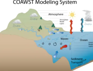
The Coupled Ocean–Atmosphere–Wave–Sediment Transport mod-eling system (COAWST; figure 2.1) is comprised of several com-ponents that include models for the ocean, atmosphere, surface waves, sediment transport, a coupler to exchange data fields. The COAWST modeling system includes only publicly-available com-ponents. The Model Coupling Toolkit (MCT) is the coupler used to exchange data fields between the ocean model ROMS, the at-mospheric model Weather Research and Forecasting (WRF), the Simulating WAves Nearshore model (SWAN), and the sediment ca-pabilities of the Community Sediment Transport Model. For this work, the ocean model ROMS and the wave driver SWAN have been coupled within the COAWST modeling system. In the follow-ing subsections a detailed description of MCT, SWAN and, ROMS is provided. In the ocean model, the wave fields are utilized to compute forcings in the form of radiation stress gradients that al-low wave-driven fal-lows, to compute Stokes velocities to provide cor-rect mass flux transport, and to compute wave-enhanced bottom stresses. The wave model receives varying water levels. The ocean surface currents - velocity from the most superficial vertical-level, i.e. the cross-shore component (us) and the longshore component

(51)

2.2 The Modeling System

Figure 2.1: The COAWST Modeling System that joins an Ocean model, an Atmosphere model, a Waves model, and a Sediment Transport Model for studies of coastal change (https:// woodshole.er.usgs.gov/operations/modeling/COAWST).

(vs), affect the wave action balance by modification of the wave

group celerity (cx + us, cy + vs) which, in turn, affects the wave

number to allow current-induced refraction.

2.2.1 The ocean model

The ocean model ROMS belongs to the general class of free sur-face, terrain-following numerical models that solve the three dimen-sional Reynolds Averaged Navier Stokes equations (RANS) using the hydrostatic and Boussinesq approximations (Shchepetkin and McWilliams 2005, 2009; Haidvogel et al. 2008) ROMS uses finite difference approximations on a horizontal curvilinear Arakawa C grid (see figure 2.2) and on a vertical stretched terrain-following coordinate. At rho-points, flow properties such as H and d are cal-culated, whereas at u-points and v-points, among the others, the components of the horizontal velocity and radiation stress are cal-culated. Momentum and scalar advection and diffusive processes

(52)

Figure 2.2: Representation of a typical ROMS grid (from Wiki ROMS).

are solved using transport equations and an equation of state com-putes the density field that accounts for temperature, salinity, and suspended-sediment contributions. ROMS provides a flexible struc-ture that allows multiple choices for many of the model components, such as several options for advection schemes (second order, third order, fourth order, and positive definite), turbulence models, lat-eral boundary conditions, bottom- and surface-boundary layer sub-models, air-sea fluxes, surface drifters, a nutrient-phytoplankton-zooplankton model, and an adjoint model for computing model inverses and data assimilation.

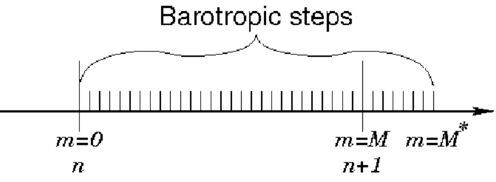
The hydrostatic primitive equations for momentum are solved using a split-explicit time-stepping scheme which requires special treatment and coupling between barotropic (fast) and baroclinic

(53)

2.2 The Modeling System

Figure 2.3: The split time stepping used in the model (Hedström 2016).

(slow) modes. A finite number of barotropic time steps (BTts),

within each baroclinic time step (BTts), are carried out to evolve

the free-surface and vertically integrated momentum equations. An integer ratio M between the time steps exists. In order to avoid the errors associated with the aliasing of frequencies resolved by the barotropic steps, but unresolved by the baroclinic step, the barotropic fields are time averaged before they replace those values obtained with a longer baroclinic step. Store weighted time means of the ubar, vbar fields centered at both time n +1₂ and time n + 1 (plus the mean water elevation ¯η at time n + 1). The latter requires

this time stepping to extend past time n + 1, using M∗ steps rather than just M (figure 2.3).

The model contains also a wetting and drying scheme to describe the evolution of the wave-averaged shoreline motion (Warner et al. 2013). The basic aspect of the wetting and drying algorithm is to compare the local value of the total water depth in each cell to a spatially-constant user-defined critical minimum depth (dcrit).

If d < dcrit, then the cell is considered to be dry and the method

only prevents outward transport of volume flux from that cell. Out-ward transport is inhibited by forcings the magnitudes of the depth-integrated momentum terms (ubar and vbar) to be zero. Further, in a dry cell the total depth is imposed to be equal dcrit. Inward

(54)

The code is written in Fortran90 and runs in serial mode on a single processor, or uses either shared- or distributed-memory architectures (OpenMP or MPI) to run on multiple processors.

2.2.2 The Wave model

SWAN is a third generation spectral wave model specifically de-signed for shallow water that solves the spectral density evolution equation (Booij, Ris, and Holthuijsen 1999). SWAN simulates wind wave generation and propagation in coastal waters and includes the processes of refraction, diffraction, shoaling, wave–wave inter-actions, and dissipation due to whitecapping, wave breaking, and bottom friction. The wave model solves the action balance equation (Holthuijsen 2010): ∂N ∂t + ∂cxN ∂x + ∂cyN ∂y + ∂cσN ∂σ + ∂cθN ∂θ = Sw σ (2.22)

where N (σ, θ, x, y, t) is the action density spectrum, σ is the rel-ative radian frequency (as observed in a frame moving with the ocean current), θ is direction normal to the wave crest, x and y are coordinate space (expressible in both spherical and Cartesian coor-dinates), and t is time. The action density is defined as the wave energy density E divided by the relative frequency (N = E/σ) and is solved because the action density is conserved in the presence of currents. The group velocities in x − and y − directions cx and cy in

the second and third terms represent the propagation of the action density in geographic space, the fourth term represents changes in relative frequency due to variations in depth and currents with a propagation speed cσ in frequency space, and the fifth term allows

depth- and current-induced refraction with a speed cθin directional

space. The Sw term represents sources and sinks of wave energy

(55)

2.3 SBCs implementation

2.2.3 The coupler

The coupler is the MCT (Jacob, Larson, and Ong 2005; Larson, Jacob, and Ong 2005) that allows for the transmission and trans-formation of various distributed data between component models using a parallel coupled approach. MCT is a program written in Fortran90 and works with the MPI communication protocol. It is compiled as a set of libraries, which are linked during the compila-tion.

During model initialization each model decomposes its own do-main into sections (or segments) that are distributed to processors assigned for that component. Each grid section on each proces-sor initializes into MCT, and the coupler compiles a global map to determine the distribution of model segments. Each segment also initializes an attribute vector that contains the fields to be ex-changed and establishes a router to provide an exchange pathway between model components.

During the run phase of the simulation the models will reach a predetermined synchronization point, fill the attribute vectors with data, and use MCT send and receive commands to exchange fields.

2.3 SBCs implementation

The 2-D ROMS Kernel adopts a predictor-corrector numerical scheme to solve the depth-averaged continuity and momentum equations. However, for this first effort toward the implementation of the SBCs, we decided to evolve our solution only at every corrector step.

Among the ROMS variables needed to calculate the SBCs, the most important are: ¯u), d and the Vertically integrated,

wave-averaged cross-shore radiation stress (hereafter S11). One of the

first problems to be faced for the calculation of the SBCs is that while ubar and d are updated at each barotropic time level, S11 is