DEPARTMENT OF INFORMATION AND COMMUNICATION TECHNOLOGY
38050 Povo — Trento (Italy), Via Sommarive 14 http://dit.unitn.it/
DO NOT BE AFRAID OF LOCAL MINIMA: AFFINE SHAKER
AND PARTICLE SWARM
Roberto Battiti, Mauro Brunato and Srinivas Pasupuleti
May 2005
Do not be afraid of local minima: Affine Shaker
and Particle Swarm
Roberto Battiti
Mauro Brunato
Srinivas Pasupuleti
Department of Computer Science and Telecommunications, Universit`a di Trento Via Sommarive 14, 38050 Povo, Trento, Italy
{battiti,brunato}@dit.unitn.it
May 2005
Abstract
Stochastic local search techniques are powerful and flexible methods to optimize difficult functions. While each method is characterized by search trajectories produced through a randomized selection of the next step, a notable difference is caused by the interaction of different searchers, as ex-emplified by the Particle Swarm methods. In this paper we evaluate two extreme approaches, Particle Swarm Optimization, with interaction be-tween the individual “cognitive” component and the “social” knowledge, and Repeated Affine Shaker, without any interaction between searchers but with an aggressive capability of scouting out local minima. The sults, unexpected to the authors, show that Affine Shaker provides re-markably efficient and effective results when compared with PSO, while the advantage of Particle Swarm is visible only for functions with a very regular structure of the local minima leading to the global optimum and only for specific experimental conditions.
1
Introduction
The problem being addressed is that of minimizing a function mapping a vector
x∈ D ⊆ Rd of d real numbers into a real number,
min
x∈D f (x)
where f : D ⊆ Rd
→ R
where d is the dimension of the domain. Furthermore, the domain of the
minimum is usually searched for within a d-dimensional interval, where
coordi-nate j is delimited by a lower bound Lj and an upper bound Uj:
D = [L1, U1] × [L2, U2] × · · · × [Ld, Ud],
where we assume that a minimum exists1.
2
Particle swarm optimization
Particle Swarm Optimization [9], PSO for short, is a population-based stochastic optimization technique for optimizing complex functions through the interaction
of individuals in a population of particles. Let’s define the notation. The
parameter d is the dimensionality of the search space, P is the total number of particles, and the position of each individual “particle” i ∈ {1, 2, . . . , P } is described by a vector xi≡ (xi1, xi2, . . . , xid). Each particle follows a trajectory
xi(t) in the search space, t ≥ 0 being the discrete iteration counter. The best
previous position (the position giving the best function value found) of the i-th
particle up to time t is referred to as pi(t) and the globally best position among
all particles in the population up to time t is called g(t). More formally, let
σi(t) ≤ t be the iteration at which particle i found its personal minimum (if the
same value was found at many iterations, then we take the first one): σi(t) ≤ t ∀s ≤ t f³xi¡σi(t) ¢´ ≤ f¡xi(s) ¢ ∀s f³xi¡σi(t) ¢´ = f¡xi(s)¢ ⇒ s ≥ σi(t).
Then the best previous position at time t for particle i is
pi(t) = xi¡σi(t)¢, i = 1, . . . , P. (1)
Similarly, let I(t) be the index of the particle which found the global best at time t (the smallest such index, in case of ties):
I(t) ∈ {1, . . . , P } ∀i = 1, . . . , P f (pI(t)(t)) ≤ f(pi(t))
∀i = 1, . . . , P f (pI(t)(t)) = f (pi(t)) ⇒ i ≥ I(t).
Then the global best coordinates at time t are
g(t) = pI(t)(t). (2)
In the following description, the components of the vector are indexed by j. The particle positions are initialized by picking points at random and with 1Note that if f is continuous then the assumption is trivial; however, even if a minimum
does not exist, the problem of computationally locating a near-infimum value of the function is still well defined.
uniform probability in an initialization range delimited by a lower bound L0 j
and an upper bound U0
j: xij ∈ [L0j, U 0
j]. Such initialization range is always
contained in the search range: Lj ≤ L0j < U
0
j ≤ Uj. In the actual usage of
the technique, if the function structure and the position of the global optimum are unknown, the initialization range coincides with the entire search range. In the tests on the benchmark functions (where for example the position of the global optimum is known to the researchers) the initialization range will be a proper subset the search range to avoid potential biases caused, for example, by symmetric initialization around a global minimum, as explained in Section 4.
Let ∆i(t) ≡ ¡δi1(t), . . . , δid(t)¢ be the “velocity” of particle i at iteration
t. The initial velocity ∆i(0) of particle i is chosen with uniform probability
within suitable limits: δij(0) = rand(−Dj, Dj). The use of the term “velocity”
and the choice of the limits will become clear in the following explanation. The discrete dynamical system governing the motion of each particle for t ≥ 1 is the following [14]:
∆i(t) = w∆i(t − 1) + c1Randd(0, 1) · (pi(t − 1) − xi(t − 1))
+c2Randd(0, 1) · (g(t − 1) − xi(t − 1)) (3)
xi(t) = xi(t − 1) + ∆i(t) (4)
where ∆i(t) is the step in the search space executed at iteration t, w is the
inertia weight [12, 13], c1 and c2 are two positive constants, and Randd(0, 1)
is a d × d diagonal matrix of independent random numbers in the range [0, 1]. Thus, each component of the position vectors is multiplied by a different random number.
An analogy from astronomy for PSO is that of a planet xi orbiting around
two “suns” given by the current best individual position (the “cognitive” com-ponent) and the current best global position (the “social” comcom-ponent). The
analogy becomes clear if ∆i(t) is interpreted as the velocity of a particle and
w is equal to 1. In this case the position of the suns determines the velocity variation, i.e., the acceleration, as forces in Physics do. Let’s note that the suns are of course changing in time, in some cases abruptly, as soon as a new best position is found either for a specific particle or for the entire swarm. A careful choice of the parameters determines the dynamics of the planets, to avoid that they get burned by the suns too early (premature convergence) or that they are spread in distant space (explosion). A detailed study of the dynamical system underlying PSO is present in [6]. The authors consider both a simplified deter-ministic dynamical system and the full stochastic system consisting of a single trajectory, with the assumption that the individual and social influence terms are fixed (i.,e., in the above analogy, that the two suns guiding the motion of the planet have a fixed position). Furthermore, no interaction among different trajectories is considered in the analysis. For the single-particle case, in the above assumptions, the analysis in fact eliminates problem-specific parameters to be fixed by the user.
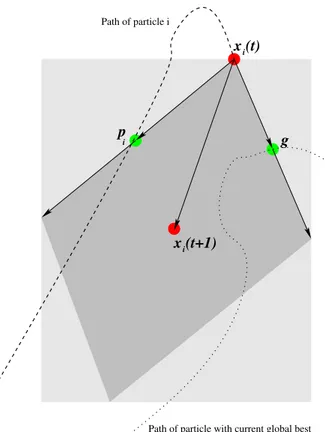
g p x (t+1) x (t) i i i Path of particle i
Path of particle with current global best
Figure 1: Particle Swarm geometry: randomized selection of the next point,
based on “attraction” by the individual best pi and global best pg. Because
each component of the two vectors is multiplied by an independent random number, the final vector can also exit the darker gray parallelogram, being only
limited by the light gray rectangle. A portion of the previous step w∆i(t − 1)
is finally added through the inertia mechanism.
values for the algorithm parameters (like c1, c2 and w), whose judicious
appli-cation can avoid the swarm explosion effect related to the deleterious effects
of randomness2. Moreover, with suitable parameter values, explosion can be
prevented while still allowing for exploration, therefore avoiding a “premature convergence” of the search.
The geometry of the position-updating equations (3) and (4) is illustrated in Fig. 1.
The specific PSO version that we consider is the one proposed in [14], where 2“the random weighting of the control parameters [. . . ] results in a kind of explosion or a
the inertia weight w is linearly varying in time as: w = w1+ (w2− w1) ·
t
MAXITER (5)
w1 and w2 are the initial and final values of the inertia weight, respectively,
t is the current iteration number and MAXITER is the maximum number of allowable iterations Following [11], we shall refer to this PSO variant as PSO-TVIW (time-variant inertia weight). This evolution in time is reminiscent of the use of an annealing schedule in the Simulated Annealing algorithm [10], where the temperature parameter is gradually reduced during the search. The pseudo-code of PSO algorithm is shown in Fig. 2.
The modulus of each component of the velocity vector of a particle (δij(t))
is limited by the maximum allowable velocity along that dimension, Dj. In the
experiment it is set to half the maximum range: Dj = (Uj− Lj)/2, the same
choice used in many papers using the same functions for comparing algorithms, in particular [11].
According to [7], by limiting the distance that can be covered in one time step to the largest dimension of the system, one avoids a possible explosion of the swarm and makes the system more robust with respect to the choice of the parameters governing its dynamics.
The step coordinates are therefore reset to the maximum allowable modulus when they exceed the limits during the iterations. In the pseudo-code, this
check and possible truncation of the step is executed by the function “limit (∆i,
(Dj))” at line 18 of Fig. 2 limiting the components of vector ∆i≡ (δi1, . . . , δid)
as follows: δij←− −Dj if δij < −Dj Dj if δij > Dj δij otherwise.
For additional possibilities to control the explosion as well as the convergence of the particles we refer the reader to the detailed analysis of [6].
3
Affine Shaker Algorithm
The Affine Shaker algorithm (or AS for short) originally proposed in [4] is an adaptive random search algorithm based only on the knowledge of function values. The term “shaker” derives from the brisk movements of the search trajectory of the stochastic local minimizer, while the term “affine” derives from the affine transformation executed on the local search region considered for generating the next point along the search trajectory.
The algorithm starts by choosing an initial point x in the configuration space and an initial search region R surrounding it, see Fig. 4. It proceeds by iterating the following steps:
1. A new tentative point is generated by sampling the local search region R with a uniform probability distribution.
Variable Scope Meaning
w1, w2, c1, c2 (input) Parameters defined in the text
P (input) Number of particles in the swarm
d (input) Dimension of the space
f (input) Function to minimize
MAXITER (input) Maximum number of iterations
D1, . . . , Dd (input) Speed limit vector
L0
1, . . . , L0d, U 0
1, . . . , Ud0 (input) Initialization range
t (internal) Iteration counter
x, ∆, p, g (internal) status vectors, defined in the text
currentvalue (internal) Function value at the current point
bestvalue (internal) Per-particle best value array
globalbest (internal) Global best value
1. function PSO TVIW (f , (L0
j), (U 0 j), (Dj), P , w1, w2, c1, c2, MAXITER) 2. t ← 0; 3. globalbest ← +∞; 4. fori ← 1 . . . P
5. xi ← initial random point in [L0
1, U 0 1] × · · · × [L 0 d, U 0 d];
6. ∆i ← initial random velocity;
7. pi ← xi; 8. currentvalue ← f( xi); 9. bestvaluei ← currentvalue; 10. ifcurrentvalue < globalbest 11. globalbest ← currentvalue; 12. g← xi; 13. whilet ≤ MAXITER 14. t ← t+1; 15. w ← w1+ (w2− w1) t MAXITER; 16. fori ← 1 . . . P 17. ∆i ← w∆i+ c1Randd·(pi− xi) + c2Randd·(g − xi); 18. limit ( ∆i, (Dj)); 19. xij ← xij + δij; 20. currentvalue ← f( xi); 21. ifcurrentvalue < bestvaluei 22. p i ← xi; 23. bestvaluei ← currentvalue; 24. ifcurrentvalue < globalbest 25. globalbest ← currentvalue; 26. g ← xi; 27. return g;
A
B
C
A’ B’
C’
Figure 3: Affine Shaker geometry: two search trajectories leading to two differ-ent local minima. The evolution of the search regions is also illustrated.
2. The search region is modified according to the value of the function at the new point. It is compressed if the new function value is greater than the current one (unsuccessful sample) or expanded otherwise (successful sample).
3. If the sample is successful, the new point becomes the current point, and the search region R is translated so that the current point is at its center for the next iteration.
The geometry of the Affine Shaker algorithm is illustrated in Fig. 3, where the function to be minimized is represented by a contour plot showing isolines at fixed values of f , and two trajectories (ABC and A’B’C’) are plotted. The pseudo-code of the algorithm is illustrated in Fig. 4. To obtain a fast and effective implementation of the above described framework it is sufficient to use a simple search region around the current point defined by edges given by a set
of linearly independent vectors R ≡ (b1, . . . , bd), and to generate a candidate
point through a uniform probability distributions inside the box. In Figure 3 search regions (in grey shade) are shown for some points in the trajectory; being in two dimensions, a couple of independent vectors defines a parallelogram centered on the point. Generating a random displacement is simple: the basis
vectors are multiplied by random numbers in the real range [−1, 1] and added:
∆=P
jrand(−1, 1)bj.
An improvement of the basic algorithm is obtained by using the double-shot strategy: if the first sample x + ∆ is not successful, the specular point
x−∆ is considered. This choice drastically reduces the probability of generating
two consecutive unsuccessful samples. The motivation is clear if one considers differentiable functions and small displacements: in this case the directional derivative along the displacement is proportional to the scalar product between displacement and gradient ∆ · ∇f. If the first is positive, a change of sign will trivially cause a negative value, and therefore a decrease in f for a sufficiently small step size. The empirical validity for general functions (not necessarily differentiable) is caused by the correlations and structure contained in most of the functions corresponding to real-world problems.
It is of interest to compare the method used for generating a new point along the trajectory with the one used in Particle Swarm. In both cases the new point is generated with uniform probability in a search frame, but in AS the frame is centered on the current point, which coincides with the best point
gencountered during the search. In fact, the current point moves only if a lower
function value if found. When a new best point is found the search frame is centered on the new point. There is no “social” component because a single searcher is active. In addition, the volume of the search frame is dynamically varied depending on the success of the last tentative move (i.e., volume becomes bigger if the last tentative move lead to a new best value, smaller otherwise), and the preferred direction of search is determined depending on the direction of the steps executed.
The design criteria are given by an aggressive search for local minima: the search speed is increased when steps are successful (points A and A’ in Fig-ure 3), reduced only if no better point is found after the double shot. When a point is close to a local minimum, the repeated halving of the search frame produces a very fast convergence of the search (point C in Figure 3). Note that another cause of reduction for the search region can be a narrow descent path (a “canyon”, such as in point B’ of Figure 3, where only a small subset of all possible directions improves the function value); however, once an improvement is found, the search region grows in the promising direction, causing a faster movement along that direction. A single run of AS run is terminated if for a predefined number S of consecutive steps one has k ∆ k< ². A sequence of S consecutive steps is considered before termination to reduce the probability that, by chance, a small step is executed because of the randomized selection and not because the point is close to a local minimum. The number of steps is set to S = 8 in the tests. The ² value is the precision with which the user wants
to determine the position of a local minimum. The default value ² = 10−6 has
been used in the tests.
By design, AS searches for local minimizers and is stopped as soon as one is found. A simple way to continue the search after a minimizer is found is to restart from a different initial random point, leading to the Repeated Affine Shaker algorithm described in Fig. 5. This leads to a “population” of AS
Variable Scope Meaning
f (input) Function to minimize
x (input) Initial point
b1, . . . , bd (input) Vectors defining search region R around x
ρe, ρr (input) Box expansion and reduction factors
d (input) Dimension of the space
t (internal) Iteration counter
P (internal) Transormation matrix
x, ∆ (internal) Current position, current displacement
1. function AffineShaker(f , x, ( bj), ρe, ρr) 2. t ← 0; 3. repeat 4. ∆ ←P jrand(−1, 1)bj; 5. iff ( x+ ∆) < f( x) 6. x← x + ∆; 7. P← I + (ρe− 1) ∆∆T k ∆ k2; 8. else if f ( x- ∆) < f( x) 9. x← x - ∆; 10. P← I + (ρe− 1) ∆∆T k ∆ k2; 11. else 12. P← I + (ρc− 1) ∆∆T k ∆ k2; 13. ∀j bj ← P bj; 14. t ← t+1
15. untilconvergence criterion;
16. return x;
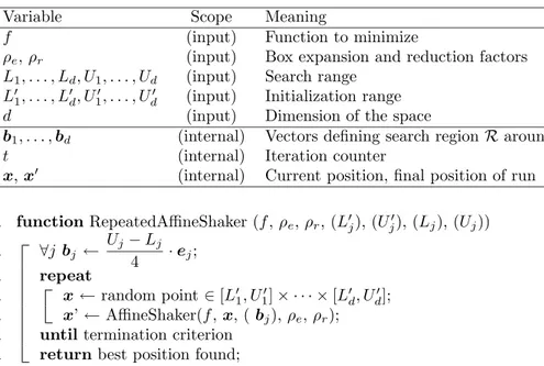
Variable Scope Meaning
f (input) Function to minimize
ρe, ρr (input) Box expansion and reduction factors
L1, . . . , Ld, U1, . . . , Ud (input) Search range
L0
1, . . . , L0d, U 0
1, . . . , Ud0 (input) Initialization range
d (input) Dimension of the space
b1, . . . , bd (internal) Vectors defining search region R around x
t (internal) Iteration counter
x, x0 (internal) Current position, final position of run
1. functionRepeatedAffineShaker (f , ρe, ρr, (Lj0), (Uj0), (Lj), (Uj)) 2. ∀j bj ← Uj− Lj 4 · ej; 3. repeat 4. x← random point ∈ [L01, U10] × · · · × [L0 d, U 0 d]; 5. x’ ← AffineShaker(f, x, ( bj), ρe, ρr);
6. untiltermination criterion
7. returnbest position found;
Figure 5: The Repeated Affine Shaker algorithm
searchers, but in this case each member of the population is independent, com-pletely unaware of what other members are doing. The range of initialization [L0
1, U10] × · · · × [L0d, U 0
d] used to generate initial random points in the tests is the
same as that used for the PSO algorithm.
While the algorithm runs, the number of function evaluations is registered, as well as the best value found. To avoid cluttering the algorithm description, these standard bookkeeping operations are not shown in the figures.
4
Benchmark optimization problems
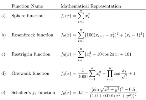
The benchmarks used for simulation are given in Table 1. We keep the same function names used in other recent PSO papers. All benchmark functions
except the Schaffer’s f6 function, which is two-dimensional, are tested with
30 dimensions. The first two functions are unimodal functions whereas the
next functions are multimodal. The global minimum value for the f1, f2, f3, f4
functions is 0.00.
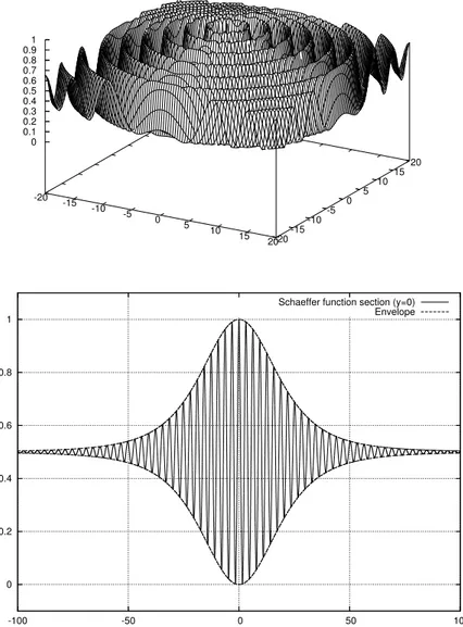
The Schaffer’s f6 function is designed to have a global maximum at the
origin, surrounded by circular “valleys” designed to trap methods based on local search, see Fig. 6. To maintain the original purpose of this test function, we maximize it. The same function is considered in [5] as a challenging problem for discrete optimization based on the hill-climbing local search and the Reactive
Search method. As it is clear from the figure, while the local structure of f6 is
-20 -15 -10 -5 0 5 10 15 20-20-15 -10-5 0 5 10 15 20 0 0.1 0.2 0.3 0.4 0.5 0.6 0.7 0.8 0.9 1 0 0.2 0.4 0.6 0.8 1 -100 -50 0 50 100
Schaeffer function section (y=0) Envelope
Figure 6: Schaffer f6function (top) and a cross-section at y = 0 (bottom). The
Table 1: Benchmarks for simulations
Function Name Mathematical Representation
a) Sphere function f1(x) = n X i=1 x2i b) Rosenbrock function f2(x) = n X i=1 ¡100(xi+1− x2i)2+ (xi− 1)2 ¢ c) Rastrigrin function f3(x) = n X i=1 ¡x2 i − 10 cos 2πxi+ 10 ¢ d) Griewank function f4(x) = 1 4000 n X i=1 x2 i − n Y i=1 cos√xi i+ 1
e) Schaffer’s f6function f6(x) = 0.5 − (sin
px2+ y2)2− 0.5
(1.0 + 0.001(x2+ y2))2
(or of the local maxima) shows a very regular structure, with a “gradient” of values clearly pointing the way towards the central optimum. From the cross section (and from simple analysis of the function) one appreciates how the knowledge of more local minima creates compelling evidence about the structure and should therefore be used by methods employing a population of interacting searchers, like PSO.
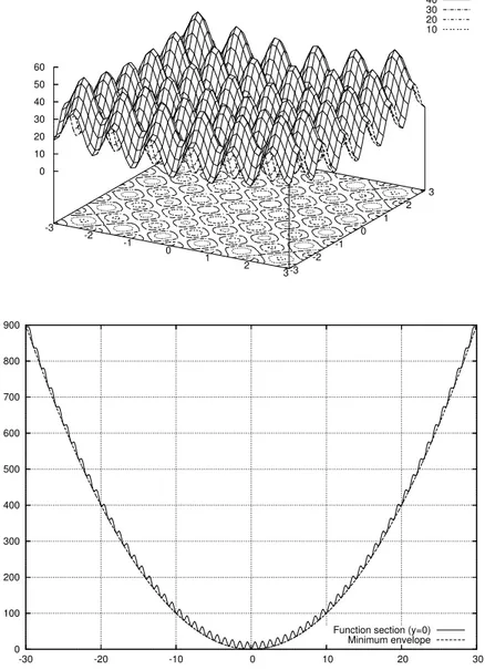
The Rastrigrin (f3) function is designed to pose similar problems to a
local-ized minimum search algorithm. As shown in Fig. 7, it exposes a plethora of proper local minima surrounding the actual global minimum in (0, 0).
For the purpose of comparison, the asymmetric initialization method used in[1, 2, 8] is adopted for initializing the population in PSO and the independent searchers in the Repeated Affine Shaker, see Table 2. The choice is motivated by [8], which shows that the typical initialization used to compare evolutionary computations can give false impressions of relative performance. In many com-parative experiments, the initial population is uniformly distributed about the entire search space which is usually defined to be symmetric about the origin. In addition, many of the test functions are crafted in such a way as to have optima at or near the origin, including the test functions for this study. This method of initialization has two potential biases when considered alone. First, if an op-erator is an averaging opop-erator involving multiple parents, such as intermediate crossover often used in evolution strategies, recombining parents from opposite sides of the origin will naturally place the offspring close to the center of the initialization region. Second, given that the location of the optima is generally not known, there is no guarantee that any prescribed initialization method will
50 40 30 20 10 -3 -2 -1 0 1 2 3-3 -2 -1 0 1 2 3 0 10 20 30 40 50 60 0 100 200 300 400 500 600 700 800 900 -30 -20 -10 0 10 20 30
Function section (y=0) Minimum envelope
Figure 7: Rastrigrin f3 function (top) and a cross-section at y = 0 (bottom).
Table 2: Search range and initialization range for the benchmark functions
Function Search range Initialization range
[L1, U1] × · · · × [Ld, Ud] [L01, U10] × · · · × [L0d, U 0 d] f1 [−100, 100]d [50, 100]d f2 [−100, 100]d [15, 30]d f3 [−10, 10]d [2.56, 5.12]d f4 [−600, 600]d [300, 600]d f6 [−100, 100]2 [15, 30]2
include the optima. Consequently, [8] suggests initializing in regions that delib-erately do not include the optima during testing to verify results obtained for symmetric initialization schemes.
When comparing the effectiveness of different optimization methods we are interested in the trade-off between computational complexity and values deliv-ered by the technique. For the values delivdeliv-ered at a given iteration we consider the best value found during the previous phase of the search (the value g in Fig. 2). To measure the computational effort we make the assumption that the evaluation of the function values at the candidate points (calculation of
f (xi)) is the dominating factor. This assumption is usually valid for significant
optimization tasks of interest for real-world problems.
The experiments are designed to model a situation where a user needs to optimize a function, has a maximum budget of computational resources to de-vote to the task or, equivalently, a maximum time budget within which the best solution found has to be delivered.
The general assumption is that no clear-cut termination criterion is avail-able. For a generic function there is no way to determine whether the global optimum has been found by the algorithm and therefore to determine when the search can be stopped. Termination is therefore dictated by exhaustion of the time/resource budget, or by obtaining a sufficiently good solution (of course a problem-specific criterion).
After evaluating the time required for a single function evaluation the max-imum number of function evaluations is derived. In selecting a technique we assume the user will prefer the one that, on average, delivers the lowest value for the given number of function evaluations. The standard deviation of the results can influence the decision if multiple runs are considered, or if the risk associated to obtaining a value that is far from the average is significant.
Because the algorithms contain a stochastic component, the value f (g) will evolve in different ways for different runs (of course the random number genera-tor seed is different for each run) and both the average and error on the average (the standard deviation of the results divided by the square root of the num-ber of tests) are reported in the tests: these data permit conclusions about the expected performance and variability of performance of the various techniques.
5
Comparison Between Particle Swarm and Affine
Shaker
In the experiments, for the PSO algorithm of Fig. 2, the constants c1and c2are
fixed at value 2.0 and the value of inertia weight w is varied from w1= 0.9 at
the beginning of the search to w2= 0.4 at the end of the search.
The experiments are conducted with different population sizes P = 10, P = 20 and P = 40. The PSO-TVIW and Repeated Affine Shaker algorithms are run for 50 trials and the average optimum value f (g) with standard devi-ation are measured as a function of the number of function evaludevi-ations. The error on the average (obtained by dividing the standard deviation of results by the square root of the number of tests plus one) has been used to assure the sta-tistical significance of the results. To avoid cluttering the plots with too much information, the plots with error on the average are presented in the Appendix. A subtle but important issue to be decided for the tests is how to fix the value of the maximum number of iterations MAXITER to derive the evolution in time of the inertia weight following equation (5). If one considers the situation encountered in the applications of a heuristic for combinatorial optimization, the user is of course not aware of the value and position of the global opti-mum (otherwise he would not need to search for it!). For most problems, even determining that a configuration is indeed the global optimum is not possible in polynomial time. These results have a strong theoretical foundation in the theory of computational complexity: if some problems could be solved in poly-nomial time, a large class of related “difficult” problems in the NP-hard class could also be solved in polynomial time, a result that is currently believed to be extremely implausible by the community of researchers in Computer Science.
The user therefore must make a reasonable allocation of computing time and be satisfied with the best solution found by the heuristic when the allotted time elapses, or repeat the search with a longer computational effort if the results are not satisfactory. In the assumption that computational effort is dominated by the number of function evaluations, for the considered PSO version this means that the user has to fix a reasonably large value of function evaluations at the beginning. The number of function evaluations in PSO is given by MAXITER · P . Therefore the MAXITER parameter is varied to get the performance of PSO for a fixed population size with respect to different number of function evaluations.
This problem is not present in the Repeated Affine Shaker: because no time-dependent parameter are present in the algorithm, the user can start the search and terminate as soon as the best value found is acceptable, or as soon as the maximum allotted time elapses.
The first series of tests, described in Section 5.1 are simulating this situation. In particular, the maximum number of function evaluations considered is fixed to 100000 for all runs.
In a second series of tests we make the assumption that an oracle is telling the correct number of function evaluations to be used by PSO on a problem.
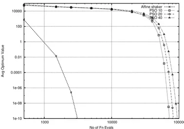
1e-10 1e-08 1e-06 0.0001 0.01 1 100 10000 1000 10000 100000
Avg Optimum Value
No of Fn Evals
Affine shaker PSO 10 PSO 20 PSO 40
Figure 8: Sphere Function f1 (fixed MAXITER)
The search is then run up to that number of function evaluations and the best final results are reported. While not realistic, this second series of tests permits to evaluate the effectiveness of PSO as a function of the choice of MAXITER, therefore providing a much larger set of experimental data. Of course, the second choice is not suggested in the applications because the computational effort is much larger: depending on the ∆M interval considered for the MAXITER value the total computational effort is the sum of the individual effort of the run up to ∆M , the independent run up to 2∆M , . . . , the run up to MAXITER. This second series of tests is presented in Sec. 5.2.
5.1
PSO versus AS, fixed maximum number of iterations
Figs. 8–13 show the comparison graphs between the Affine Shaker and PSO algorithm for the different benchmark functions considered. The plots are on a log-log scale to show the evolution over a very wide range of values and for up to a large number of function evaluations. In the Appendix Fig. 20–25 show the same comparison graphs but with error of the average included.
For all functions apart from the Schaffer f6, the Repeated Affine Shaker finds
very rapidly low values of f and it tends to maintain the advantage even for large number of iterations. Better values are found by PSO only in the second part of the search (after about 50000 function evaluations).
For the f6 function, if one consider minimization (and therefore is looking
for a point at the bottom of the first circular ring surrounding the needle at the origin) Repeated Affine Shaker lags behind PSO in the initial phase but rapidly and consistently catches up after about 20000 function evaluations, see Fig. 12. If one considers maximization, see Fig. 13 where the difference from
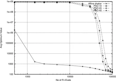
100 1000 10000 100000 1e+06 1e+07 1e+08 1e+09 1000 10000 100000
Avg Optimum Value
No of Fn Evals
Affine shaker PSO 10 PSO 20 PSO 40
Figure 9: Rosenbrock Function f2(fixed MAXITER)
10 100 1000
1000 10000 100000
Avg Optimum Value
No of Fn Evals
Affine shaker PSO 10 PSO 20 PSO 40
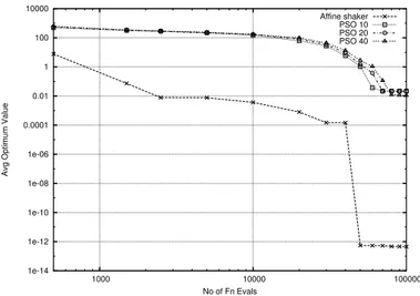
1e-14 1e-12 1e-10 1e-08 1e-06 0.0001 0.01 1 100 10000 1000 10000 100000
Avg Optimum Value
No of Fn Evals
Affine shaker PSO 10 PSO 20 PSO 40
Figure 11: Griewank Function f4 (fixed MAXITER)
0.0001 0.001 0.01 0.1
1000 10000 100000
Avg Optimum Value
No of Fn Evals
Affine shaker PSO 10 PSO 20 PSO 40
0.0001 0.001 0.01 0.1
1000 10000 100000
One minus Avg Optimum Value
No of Fn Evals
Affine shaker PSO 10 PSO 20 PSO 40
Figure 13: Schaffer Function Maximizingf6(fixed MAXITER)
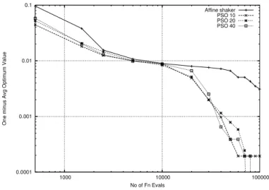
the optimum 1 − f(g) is shown, Affine Shaker is lagging at the beginning, providing similar good quality values (within 0.01 of the maximum) at about 10000 function evaluations, and then showing a slower improvement during the
final part of the search. Considering the structure of the f6function, maliciously
designed to trap methods based on hill-climbing, with a local optimum at the center surrounded by a very small attraction basin (the “needle” in Fig. 6), these results are hardly surprising. In fact, PSO is influenced by the envelope of the function, see again Fig. 6, that is clearly showing the way towards the global optimum, while Affine Shaker without any interaction starts each search by hoping that random extraction of trajectory points will by chance fall inside the “needle” at the center.
While the plots show the entire story, to simplify the comparison and to consider another measure based on average time required by a run to reach a threshold value, it is useful to select some fixed threshold and to measure what is the average number of function evaluations used by the different algorithms to reach the thresholds. Table 3 list the number of function evaluations while Table 4 show the relative numbers, as speedup of AS with respect to PSO.
It can be noted that, for the chosen thresholds, Affine Shaker consistently provides a substantial speedup with respect to PSO.
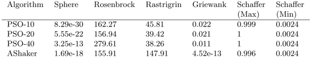
Finally, a third measure of performance is obtained as the average value found by the two methods at the end of the 100000 function evaluations. These results are collected in Table 5. Again, Affine Shaker is better than or compara-ble to PSO in all cases apart from the Rastrigrin function which shows a clear advantage for PSO.
Table 3: Function Evaluations
Algorithm Sphere Rosenbrock Rastrigrin Griewank Schaffer (goal) (< 0.1) (< 10000) (< 200) (< 0.2) (Max, > 0.99)
AShaker 1500 1040 15410 1500 2140
PSO-10 55370 53580 40750 55850 3830
PSO-20 61370 58880 42460 61200 4160
PSO-40 68530 66410 46790 68410 3940
Table 4: Speed-Up Table
Algorithm Sphere Rosenbrock Rastrigrin Griewank Schaffer (Max)
PSO-10 37 51 2.6 37 1.79
PSO-20 41 57 2.7 41 1.94
PSO-40 46 64 3 45 1.84
AShaker 1 1 1 1 1
Table 5: Average Optimum Value at the end of 100000 Function Evaluations
Algorithm Sphere Rosenbrock Rastrigrin Griewank Schaffer Schaffer (Max) (Min)
PSO-10 8.29e-30 162.27 45.81 0.022 0.999 0.0024
PSO-20 5.55e-22 156.94 39.42 0.021 1 0.0024
PSO-40 3.25e-13 279.61 38.26 0.011 1 0.0024
1e-10 1e-08 1e-06 0.0001 0.01 1 100 10000 1000 10000 100000
Avg Optimum Value
No of Fn Evals
Affine shaker PSO 10 PSO 20 PSO 40
Figure 14: Sphere Function f1
5.2
PSO versus AS, variable maximum number of
itera-tions
As mentioned, this second series of tests presents the same data for the Affine Shaker, while it reports end values obtained by multiple runs of PSO up to different values of maximum iterations (or, equivalently, maximum number of function evaluations). For each data point at a given number of function eval-uations 50 independent runs of PSO are executed. The points on the plots are connected for better visibility but refer to different experimental runs, where the oracle gives a different MAXITER value.
Even in the case that help by the oracle is used by PSO, it can be observed that the Repeated Affine Shaker algorithm takes considerably less number of function evaluations to find comparable values when compared to PSO with
dif-ferent population sizes for the functions f1, f2, and f4. This result is consistent
for different thresholds put on the value to be reached.
Given the simplicity of the Repeated Affine Shaker, without any interaction among the multiple runs, these results were unexpected, in particular for the
more complex f2 and f4 functions.
For the Rastrigrin f3 and Schaffer f6 the situation is more varied. For f3
AS finds very rapidly good local minima, while PSO finds better values for a fixed number of function evaluations if one searches for lower values, see Fig. 16. When the Schaffer function is considered, both minimization and maximization are more rapid for PSO.
100 1000 10000 100000 1e+06 1e+07 1e+08 1e+09 1000 10000 100000
Avg Optimum Value
No of Fn Evals
Affine shaker PSO 10 PSO 20 PSO 40
Figure 15: Rosenbrock Function f2
10 100 1000
1000 10000 100000
Avg Optimum Value
No of Fn Evals
Affine shaker PSO 10 PSO 20 PSO 40
1e-14 1e-12 1e-10 1e-08 1e-06 0.0001 0.01 1 100 10000 1000 10000 100000
Avg Optimum Value
No of Fn Evals
Affine shaker PSO 10 PSO 20 PSO 40
Figure 17: Griewank Function f4
0.0001 0.001 0.01 0.1
1000 10000 100000
Avg Optimum Value
No of Fn Evals
Affine shaker PSO 10 PSO 20 PSO 40
0.0001 0.001 0.01 0.1
1000 10000 100000
One minus Avg Optimum Value
No of Fn Evals
Affine shaker PSO 10 PSO 20 PSO 40
Figure 19: Schaffer Function Maximizingf6
6
Conclusions
This paper compares two stochastic local search techniques for the minimiza-tion of continuous funcminimiza-tions. Both techniques generate a search trajectory by producing the next point through a randomized extraction in a localized region, and both consider multiple trajectories, but they differ in a radical manner in the amount of interaction among the different searchers. In one case (Re-peated Affine Shaker), the different searchers are independent, no information is transferred from one trajectory to another one. Running searches in parallel or sequentially produces the same results. In the other case (Particle Swarm), each trajectory is influenced also by the collective information derived by the other trajectories. Because of the larger amount of information available in the second case and the possibility to “intensify” the search in promising regions, one expects a much larger efficiency. The experiments are designed to simulate a situation where a user selects a large number of iterations before starting the search (not knowing a priori the appropriate number of function evaluations needed to reach acceptable results) and a different situation in which an oracle tells the user the appropriate MAXITER value. Let’s note that intermediate cases can also be considered, so that the user is ignorant at the beginning but progressively tunes parameters depending on preliminary results, the detailed examination of this context is considered in an extension of this research.
The experimental results are unexpected: in the first experimental setting Affine Shaker tends to provide significantly better results in a much smaller number of function evaluations in many conditions, while PSO demonstrates an
advantage only for Rastrigrin f3at the end of the search and for the “malicious”
sug-gests the appropriate value for the maximum number of iterations to run PSO with, for some functions, AS gives better results, or reaches a given result with a smaller number of function evaluations, in other cases PSO has a better per-formance. When PSO has a significantly better performance, a closer analysis reveals that the function structure is “designed” so that the values of the local minima in space clearly point the way towards the global optimum.
Interestingly enough, similar results related to the need to specify the evo-lution in time of a parameter guiding the search have been found in a very different context related to comparing Simulated Annealing and Tabu Search on the Quadratic Assignment Problem [3].
A tentative conclusion of this preliminary work is that the effort to avoid a premature convergence of the swarm causes a performance penalty in particular in the initial part of the search, when good local minima can be lost because the particles are moving with high velocity over a portion of the search region (the “fear of local minima” effect if we want an analogy). The second technique (AS) is very aggressive in searching for local minima: rapid convergence is desired because diversification can be obtained with the simple multi-start technique.
Given the remarkable performance of the simple AS strategy it is of course of interest to consider integration of swarm intelligence methods with AS, to see whether adding interactions between the individual searchers by Particle Swarm methodologies will provide even better results. A second issue of relevance is to extend the results obtained on a selected number of carefully selected functions to a wider selection of functions with a more complex and “unpredictable” structure. The two issues are currently investigated in our group.
Acknowledgement
We acknowledge support by the WILMA project funded by the Autonomous Province of Trento, and by the QUASAR project funded by MIUR.
References
[1] P. J. Angeline. Evolutionary Optimization versus Particle swarm opti-mization:philosophy and performance difference. Annual Conference on Evolutionary Programming, 1998.
[2] P. J. Angeline. Using Selection to Improve Particle Swarm Optimizaation. IEEE International Conference on Evolutionary Computation, May 1998. [3] R. Battit and G. Tecchiolli. Simulated annealing and tabu search in the
long run: a comparison on QAP tasks. Computer and Mathematics with Applications, 28(6):1–8, 1994.
[4] R. Battiti and G. Tecchiolli. Learning with first, second and no derivatives: A case study in high energy physiscs. Neurocomp, 6:181–206, 1994.
[5] Roberto Battiti and Giampietro Tecchiolli. The reactive tabu search. ORSA Journal on Computing, 6(2):126–140, 1994.
[6] M. Clerc and J. Kennedy. The particle swarm – explosion, stability, and convergence in a multidimensional complex space. IEEE Transactions on Evolutionary Computation, 6(1):58–73, 2002.
[7] R. C. Eberhart and Y. H. hi. Comparing inertia weights and constriction factors in particle swarm optimization. Proc. IEEE Int. Congr. Evolution-ary Computation, 1:84–88, 2000.
[8] D. Fogel and H. G. Beyer. A Note on the Empirical Evaluation of Inter-mediate Recombination. Evolutionary Computation, 3(4), 1995.
[9] Kennedy J. and Eberhart R.C. Particle Swarm Optimization. IEEE Int. Conf. Neural Networks, pages 1942–1948, 1995.
[10] S. Kirkpatrick, C. D. Gelatt, and M. P. Vecchi. Optimization by Simulated Annealing. Science, 220:671–680, 1983.
[11] A. Ratnaweera, S.K. Halgamuge, and H.C. Watson. Self-organizing hierar-chical particle swarm optimizer with time-varying acceleration coefficients. IEEE Transactions on Evolutionary Computation, 8(3):240–255, 2004. [12] Y. H. Shi and R. C. Eberhart. A Modified Particle Swarm Optimizer. IEEE
International Conference on Evolutionary Computation, May 1998. [13] Y. H. Shi and R. C. Eberhart. Parameter Selection in Particle Swarm
Optimization. Annual Conference on Evolutionary Programming, March 1998.
[14] Y. H. Shi and R. C. Eberhart. Empirical study of particle swarm opti-mization. Proc. IEEE Int. Congr. Evolutionary Computation, 3:101–106, 1999.
7
Appendix
Results for a fixed number of 100000 function evaluations with error bars (error on the average) are illustrated in Fig. 20–25, while results related to an oracle specifying the number of function evaluations to use in PSO are reported in Fig. 26–31. 1e-10 1e-08 1e-06 0.0001 0.01 1 100 10000 1000 10000 100000
Avg Optimum Value
No of Fn Evals
Affine shaker PSO 10 PSO 20 PSO 40
100 1000 10000 100000 1e+06 1e+07 1e+08 1e+09 1000 10000 100000
Avg Optimum Value
No of Fn Evals
Affine shaker PSO 10 PSO 20 PSO 40
Figure 21: Rosenbrock Function f2
10 100 1000
1000 10000 100000
Avg Optimum Value
No of Fn Evals
Affine shaker PSO 10 PSO 20 PSO 40
1e-14 1e-12 1e-10 1e-08 1e-06 0.0001 0.01 1 100 10000 1000 10000 100000
Avg Optimum Value
No of Fn Evals
Affine shaker PSO 10 PSO 20 PSO 40
Figure 23: Griewank Function f4
0.0001 0.001 0.01 0.1
1000 10000 100000
Avg Optimum Value
No of Fn Evals
Affine shaker PSO 10 PSO 20 PSO 40
0.0001 0.001 0.01 0.1
1000 10000 100000
One minus Avg Optimum Value
No of Fn Evals
Affine shaker PSO 10 PSO 20 PSO 40
Figure 25: Schaffer Function Maximizingf6
1e-10 1e-08 1e-06 0.0001 0.01 1 100 10000 1000 10000 100000
Avg Optimum Value
No of Fn Evals
Affine shaker PSO 10 PSO 20 PSO 40
100 1000 10000 100000 1e+06 1e+07 1e+08 1e+09 1000 10000 100000
Avg Optimum Value
No of Fn Evals
Affine shaker PSO 10 PSO 20 PSO 40
Figure 27: Rosenbrock Function f2
10 100 1000
100 1000 10000 100000
Avg Optimum Value
No of Fn Evals
Affine shaker PSO 10 PSO 20 PSO 40
1e-10 1e-08 1e-06 0.0001 0.01 1 100 10000 1000 10000 100000
Avg Optimum Value
No of Fn Evals
Affine shaker PSO 10 PSO 20 PSO 40
Figure 29: Griewank Function f4
0.0001 0.001 0.01 0.1
1000 10000 100000
Avg Optimum Value
No of Fn Evals
Affine shaker PSO 10 PSO 20 PSO 40
0.0001 0.001 0.01 0.1
1000 10000 100000
One minus Avg Optimum Value
No of Fn Evals
Affine shaker PSO 10 PSO 20 PSO 40