S H A D O W E C O N O M Y: A N E U R A L N E T W O R K A P P R O A C H
a n d r e a m e r l o
f a c u lt y s u p e r v i s o r: Prof. Giorgio Buttazzo
Sant’Anna School of Advanced Studies Information and Industrial Engineering
Diploma di Licenza Magistrale December 2018
Andrea Merlo:
Shadow Economy: A Neural Network Approach, Diploma di Licenza Magistrale, © December 2018
s u p e r v i s o r s:
Prof. Giorgio Buttazzo
l o c at i o n:
Gothenburg, Sweden Rome, Italy
C O N T E N T S
i i n t r o d u c t i o n 1
1 i n t r o d u c t i o n 2
1.1 Time and Location . . . 2
1.2 Shadow Economy . . . 2
1.2.1 Definition . . . 3
1.2.2 Issue: Size and Complexity . . . 4
1.3 Purpose and Problem Statement . . . 6
1.4 Thesis Outline . . . 7
2 l i t e r at u r e 8 2.1 Past Studies . . . 8
2.1.1 Causes and Indicators . . . 8
2.1.2 Unconventional Causes . . . 11
2.1.3 Measurements and Size . . . 11
2.2 Motivation and Objectives . . . 13
2.2.1 Why Neural Networks? . . . 14
3 d ata a n d m e t h o d o l o g y 15 3.1 Source Data . . . 15 3.2 Methodology . . . 26 3.2.1 Software Stack . . . 27 ii a na ly t i c a l m e t h o d s 28 4 u n s u p e r v i s e d l e a r n i n g 29 4.1 Classification . . . 29 4.1.1 Data Selection . . . 29 4.1.2 K-Means Clustering . . . 30
4.1.3 Partition Around Medoids . . . 38
4.2 Data Reduction . . . 43
4.2.1 Dimension Reduction . . . 43
4.2.2 PCA . . . 44
4.2.3 Hopfield Neural Network . . . 49
4.2.4 Autoencoder . . . 53 4.2.5 Application . . . 54 4.3 Visualization . . . 59 5 s u p e r v i s e d l e a r n i n g 60 5.1 Classical Methods . . . 60 5.1.1 MIMIC Method . . . 60 5.1.2 Model Selection . . . 61
5.1.3 MIMIC Method on Reduced Data . . . 63
5.2 Neural Network Methods . . . 63
5.2.1 Multilayer Perceptron . . . 63
5.3 Results . . . 66
5.3.2 MIMIC . . . 67 5.3.3 MLP . . . 68 5.3.4 Model # 1 . . . 71 5.3.5 Model # 2 . . . 71 5.3.6 Comparison . . . 72 iii r e s u lt s a n d c o n c l u s i o n s 73 6 c o m pa r i s o n s, results and conclusions 74 6.1 Comparative Results . . . 74
6.1.1 Shadow Economy Benchmark . . . 74
6.1.2 Full Neural Flow . . . 75
6.2 Conclusions . . . 75
L I S T O F F I G U R E S
Figure 1 Distance matrix for years 2016, 2012, 2008 and 2004. . . 30
Figure 2 WSS of K-Means clustering on year 2014. . . 31
Figure 3 WSS of K-Means clustering on year 2014. . . 32
Figure 4 WSS of K-Means clustering on year 2016. . . 33
Figure 5 WSS of K-Means clustering on year 2002. . . 34
Figure 6 K-Means average silhouette width for year 2014. . . 35
Figure 7 K-Means cluster analysis for years 2004, 2008, 2012 and 2016. . . 36
Figure 8 K-Means cluster pattern analysis for the entire period. 38 Figure 9 Average Silhouette Width as a function of medoids. . . 39
Figure 10 Silohuette width for each country. . . 40
Figure 11 Cluster representation over principal components. . . . 41
Figure 12 PAM cluster pattern analysis for the entire period. . . . 43
Figure 13 Scree plot for the eigenvalues of PCA analysis. . . 46
Figure 14 Qor for PCA analysis. . . 47
Figure 15 Variable contributions in PCAs. . . 48
Figure 16 Variable contributions in selected PCAS. . . 49
Figure 17 Self Organizing Map Architecture. . . 50
Figure 18 SOM codes on grid. . . 51
Figure 19 Counts of data object per SOM cell. . . 52
Figure 20 SOM heatmap for the most relevant input variables in PCA analysis. . . 53
Figure 21 Autoeconder Structure. . . 54
Figure 22 Autoeconder Generalized Weight for Neuron 1 (a). . . 55
Figure 23 Autoeconder Generalized Weight for Neuron 1 (b). . . 56
Figure 24 Autoeconder Generalized Weight for Neuron 1 (c). . . 57
Figure 25 Autoeconder Generalized Weight for Neuron 1 (d). . . 58
Figure 26 MLP Structure. . . 64
Figure 27 MLP SSE on Different Architecture . . . 69
Figure 28 MLP Architecture . . . 71
Figure 29 MLP Generalized Weights for traOpe, gdpCapCur, em-pRatTot and expSha . . . 71
Figure 30 MLP Generalized Weights for polSta, rulLaw, conCor . 71 Figure 31 MLP Architecture . . . 71
Figure 32 MLP Generalized Weights for traOpe, gdpCapCur, agrGdp, taxPay . . . 71
Figure 33 MLP Generalized Weights for neet19, aduEduLevTry, socSpePub . . . 71
L I S T O F TA B L E S
Table 1 Categorization of the Underground Economy . . . 4
Table 2 Size of the shadow economy (% of official GDP) in 21 OECD countries . . . 5
Table 3 Causes and Indicators Variable . . . 10
Table 4 Sources databases . . . 15
Table 5 Selected Countries . . . 16
Table 6 Data Source Abbreviations . . . 26
Table 7 K-Means clustering results over the entire period. . . . 37
Table 8 PAM clustering results over the entire period. . . 42
Table 9 PCA Eigenvalues and variance for each dimension. . . 45
Table 10 Autoencoder generalized weight norms . . . 59
Table 11 MIMIC Models Proposed . . . 62
Table 12 MIMIC Models Proposed on PCA reduced data . . . . 63
Table 13 MIMIC Models Proposed on Autoencoder Reduced Data 63 Table 14 Panel Integrity Matrix . . . 66
Table 15 MIMIC Results with Model # 1, # 2 and # 3 . . . 68
Table 16 MLP Results. (*) averaged over 50 iterations, (**) best over 50 iterations. . . 71
Table 17 MLP Results . . . 72
Table 18 Shadow Economy Estimates from CESifo. . . 74
Table 19 MLP Results . . . 74
Table 20 Shadow Economy Estimates based on MIMIC Method 74 Table 21 Shadow Economy Estimates derived from MLP . . . . 75
Part I
1
I N T R O D U C T I O N
In this introduction Chapter the project background, aim and purposes will be explained, in addition the thesis structure will be outlined. In particular we will:
1. Location and period in which this project has been worked out 2. Introduction to the project theme and background
3. Purposes and objectives of the project 4. Thesis outline
1.1 t i m e a n d l o c at i o n
This thesis has been carried out under the supervision of Prof. Giorgio But-tazzo, Full Professor of Computer Engineering at Scuola Superiore Sant’Anna of Pisa.
The project has been worked out during my stay in Sweden due to working experience in Gothenburg and during last month in Rome.
1.2 s h a d o w e c o n o m y
Shadow Economy collects all these economic activities in which a certain amount of goods or money is exchanged, and which are not regulated by any laws, but which are only regulated by the participants themselves. To the extent of some people, these activities are free economic activities: free from any regulations on what could be done and what could not be done, as for example illegal activities prohibited by the law, and free from any control or accounting, thus no tax is paid [52].
The issue of Shadow Economy, concerning both the topics of how to mea-sure, understand and chase it, has been relatively important during the past two decades in respect of before and it has seen relevant policy implications in developed countries. Shadow Economy is problematic for several reasons, including the following ones:
• There is a fundamental need to establish a unique regulated and control framework in which any units could issue an economical transaction. This framework should easily allow units to freely join or leave and to securely puts in place their exchanges. As in contrast with what stated in the first paragraph, rules should be formalized both on the rightness and the accounting side.
• The framework in which regular economic takes place should educate people on the purposes of taxation and acting in a regulated environ-ment. These should not only include all the public goods provided with the incomes of taxes, but the rights that any units in the regular economic has and the legal framework which allows for a more equal interactions between them. Operating in the shadow economy could possible lead to relationships marred by violence and inequalities, by bypassing legal institutions.
• Looking at the overall picture, an higher rate of shadow economy in respect of regular one means an higher tax burden for the latter, which has been shown lead to an higher rate of migration from the shadow to the formal one.
1.2.1 Definition
In several papers and works the term shadow economy had usually com-prised different activities: one has to distinguish between goods and services produced and consumed within the household, ‘soft’ forms of illicit work (‘moonlighting’), and illegal employment and social fraud, as well as crimi-nal economic activities [52].
Owing to this fact, the EU Commission initiated a standardisation on the European level that is being supported by extensive studies on the gross national product of EUROSTAT. The proposed definition of "Non-observed Economy" (NOE) is [21]:
Non-observed economy (NOE) refers to all productive activities that may not be captured in the basic data sources used for compiling national ac-counts. The following activities are included: underground, informal (includ-ing those undertaken by households for their own final use), illegal, and other activities omitted due to deficiencies in the basic data collection pro-gram. The term ‘non-observed economy’ encompasses all of these activities and the related statistical estimation problems.
By referring to the five set of activities introduced by the definition, we could characterize them trough the following descriptions [26]:
• Underground production: activities that are productive and legal but are deliberately concealed from public authorities to avoid payment of taxes or compliance with regulations.
• Informal sector production: productive activities conducted by unin-corporated enterprises in the household sector or other units that are unregistered and/or less than a specified size in terms of employment, and that have some market production.
• Production of households for own-final use: productive activities that result in goods or services consumed or capitalized by the households that produced them.
• Illegal production: productive activities that generate goods and ser-vices forbidden by law or that are unlawful when carried out by unau-thorized procedures.
• Statistical underground: defined as all productive activities that should be accounted for in basic data collection programmes but are missed due to deficiencies in the statistical system.
Looking at the activities with more details we would have to better under-stand if all economic transactions derived from the above definition could be included in the shadow economy. A parallel definition for underground economy could be stated as [52]:
The term underground economy comprises all goods and services which normally should be added to the calculation of the national product but are not part of the latter for certain reasons.
Criteria Underground Informal Household Illegal (and Criminal)
Production Legal Legal Legal Illegal
Transaction Yes Yes No Yes
Output Legal Legal Legal Legal/Illegal
Examples
TODO: Add examples
Table 1: Categorization of the Underground Economy
Following the latest definition, illegal activities are not included in this analysis, in fact the difference between the "illegal" or "criminal" sector and the "informal" one derives from the fact that production/ distribution and output of criminal activities are illegal. On the other hand, an activity in the irregular sector becomes part of the shadow economy only if the distribution and the production is illegal, since the output is legal [56].
1.2.2 Issue: Size and Complexity
Starting from the initial papers in the 80’s, several authors introduced dif-ferent methods to measure the size of shadow economy, leading to difdif-ferent results. We could state three different approach: direct approach [28],
approach [17]. We will later discuss about them in Section ??, so now we will
focus on the results that they brought up.
In this work we will mainly focus on OECD countries, thus results of find-ing about these countries reveal that, since the 1990s, the size of shadow economy has decreased. If we look at the unweighted average for all coun-tries during the 90s it was 17 %, number which dropped to 14 % in 2007. Table ?? presents these findings for the 21 OECD cuntries from the 90s to 2012[7].
TODO: Add all data to table
OECD Countries Shadow Economy 1989/90 1994/95 1997/98 1999 2001 2003 2005 2007 2009 2011 2012 Australia 10.1 13.5 14.0 14.4 14.3 13.9 13.7 13.5 - - -USA 6.7 8.8 8.9 8.8 8.8 8.7 8.5 8.4 - - -Average - - -
-Table 2: Size of the shadow economy (% of official GDP) in 21 OECD countries
In these finding we could clearly see five different sets of countries, which differentiate themselves not only on the absolute size of the shadow economy, but on the their trend during the 90s and 00s:
• Southern European Countries: Greece, Italy, Portugal and Spain. These are the countries with the higher ratio of shadow economy in respect of the GDP, approximate 20-30 %. The related tax burden and size of the state greatly affects these countries [7]. However from 2007 data
shows that they were able to reduce the shadow economy rate by 14.5 % (2007-2012 period).
• Nordic Countries: Denmark, Finland, Ireland, Netherlands, Norway and Sweden. These countries shows an higher then the average (OECD average) shadow economy rate. Although high quality standards and a working welfare state is put in place in this region, all these coun-tries suffer from an high tax burden with relatively light regulatory burden [7]. They, as the Southern European Set, showed a considerable
reduction of the shadow economy after 2007, roughly 22 % (2007-2012 period).
• Central European Countries: Belgium, France and Germany. These coun-tries shows an OECD average shadow economy rate and slightly less reduction in this rate between 2007 and 2012 as others did.
• High Tax Morale: Japan, Switzerland and USA. This set of countries clearly shows an under average shadow economy rate, it is mainly due an higher tax-moral from his/her citizenship and a low level of regula-tion.
• Others: Australia, Austria, Canada, Uk. These countries are the ones with the highest share of GDP and wellness which show a slight in-crease in the shadow economy size during this period.
Looking at the size and the complexity of the Shadow Economy, it is im-portant to get access to the right tools in order to measure and understand it. In recent years, its growth and large size have brought up the issue at istitu-tion level more often then in the past, thus raising rightful popular concern on the issue has emerged [52].
The issue of measure and understand shadow economy could be related to the problem of study a complex system and its interactions. Previous works addressed the issue with this focus in mind, trying to put in place other knowledge coming from other social science discipline [10]. A "complex
sys-tem" in general is a group or organization which is made up of many interact-ing parts. Archetypal complex systems include the global climate, economies, ant colonies, and immune systems [44]. Nowadays methods to address the
issue do not take into account this complexity, thus they lack an effective framework to properly get the overall picture.
Studies in this direction aimed to use tools from other social sciences in order to tackle the problem. The "Structural Equation Modeling" has been proposed in order to take into account the "unobserved variable" which in this case is the shadow economy. In such a complex system is not possible to study its sole components in order to get the overall picture, but it is neces-sary to study the system as a hole and it is not possible to further simplify it in order to deal with simpler units [10].
Due to the complexity of the problem and the difficulties that many studies faced in order to establish relations and mechanisms behind the shadow economy, be able to study the issue with more powerful tools could reveal links never observed before. This indeed would contribute to the set of inputs that economists and policy makers have in order to tackle the problem from a normative point of view [52].
1.3 p u r p o s e a n d p r o b l e m s tat e m e n t
From what stated in the previous paragraph, the problem statement can be formulated as:
The focus of the work is to analyze and review the use of neural network approaches to a traditional macroeconomic topic such as shadow economy. The work entails including dimension reduction and classification of het-erogeneous input data, towards the characterization, in terms of prediction, of several classical and neural networks strategies to establish connection between macroeconomic variables and shadow economy in a set of OCED countries during a finite time span.
1.4 t h e s i s o u t l i n e
The thesis is structured as follow: [TODO]
c h a p t e r 2 Chapter 2 presents a brief overview of classical measurement methods available in literature in order to tackle the shadow economy esti-mation problem. These will imply both direct and indirect approaches. In addition key studies will be reviewed.
c h a p t e r 3 Chapter 3 presents all the panel data that will be used trough this work, including a brief explanation of their usage.
c h a p t e r 4 In Chapter 4 classification and reduction methods will be pre-sented, including classical and neural approaches. Hints and reduced data would be further used in the final part of the work.
c h a p t e r 5 In Chapter 5 several regression and prediction methods will be outlined and derived, including classical and neural approaches. An initial comparison between the twos would be presented.
c h a p t e r 6 Chapter 6 concludes the work and provide benchmark figures against real world data on shadow economy.
2
L I T E R AT U R E
In this Chapter the analyzed literature and past studies are reviewed and traditional approach are presented. In conclusion we highlight the features why we opted for a Neural Network approach. In details:
1. Past studies review and listing of causes and indicators determining shadow economy
2. Classical indirect and direct approaches such as physical input method are presented
3. Motivations behind the work
4. Neural Network focus and clarification of theirs role toward the work
2.1 pa s t s t u d i e s
2.1.1 Causes and Indicators
It is important to understand the main determinants of the shadow economy because firstly many models are based on those, as the MIMIC one, and sec-ondly it could give hints on how to solve or mitigate the issue.
Starting from Allingham and Sandmo, tax compliance depends on its ex-pected costs and benefits. All metrics are included in this framework where each economic unit acts in order to achieve an individual marginal tax rate by leveling non-compliance costs and true individual income [2].
The literature highlights specific causes and indicators of the shadow econ-omy, in particular in Table 3 the main causes and indicators determining
shadow economy are presented and briefly discussed. In addition for each of them the most relevant past studies are referred.
Variable Description and Background References
(1) Overall Tax burden
As the overall tax burden we include each com-ponents which constitute the total amount of taxes payed by an individual or a company. Thus here we list tax on payroll, tax on goods and service, tax on corporate profits, tax on in-come and tax on property. In particular previ-ous study has highlight the fact that the bigger the difference between the total labor cost in the official economy and after-tax earnings, the greater the incentive to reduce the tax wedge and work in the shadow economy.
[]
(2) Social Secu-rity Contribu-tions
Share of payment that goes in social security contributions with respect to the overall tax burden greatly influence the choice of an indi-vidual in join official economy.
[]
(3) Non Compli-ant Costs and De-terrence
In this context we often end up in a situa-tion which is difficult to empirically evaluate as there is no shared data on legal framework and structure at international level. However survey methods has shown that the perceived risk of detention poses a major threats to the in-dividual in respect of fines and punishments. (4) Quality of
In-stitutions
Quality of institutions and the perception of public services play a key factor in the adher-ence to the official economy. An highly cor-rupt government tends to be associated with a larger unofficial activity, in addition a certain level of taxation, mostly spent in productive public services, characterizes efficient policies. In fact, production in the formal sector bene-fits from higher provision of productive public services and is negatively affected by taxation, while the shadow economy reacts in the oppo-site way.
[]
(5) Morality Here we principally refer to tax morale, and the moral behind the choise to adhere to the official economy and regularly pay taxes. Tax morale in specific country holds even in case of bad and non efficient public services, as it is seen as the sole tool for an equal redistribution of wellness. In addition tax morale is stronger in countries where individuals are seen as part-ner from the authority, and not as clients.
(6) Regulations A country with an heavier set of regulations tends to have a greater amount of barriers in entering official economy. In facts they leads to a substantial increase in labor costs: thus coun-tries that are more heavily regulated tend to have a higher share of the shadow economy in total GDP.
[]
(7) Development of the official economy
The status of the official economy does play a role in the individual perception and its ince-tive in working in the shadow economy. The development of the official economy coulbe be measured as the GDP growth or the unemploy-ment quota.
[]
(8) Agriculture Sector
Previous study has shown how a larger agri-culture sector could influece shadow economy partecipation, thus fostering it. The agriculture sector could be measured via its share in GDP and its share in the employment ratio.
[]
(9) Economic
Composition
In a more general prospective the overall com-position of economy plays a consistent role in the share of shadow economy. In particular we will consider trade openness as a measure of the probability for an arised of a illegal trade inside the country.
[]
Indicators
(1) Use of cash The larger the shadow economy, the more cash will be used in order to fund the illegal activ-ities. Here M1/M2 or currency exchange ratio is used as a proxy.
(2) Share of labor force
The higher the shadow economy, the lower the official labor force participation rate.
(3) GDP per
capita
A growth in the shadow economic activities should be reflected in to the official economy. Here the GDP per capita growth is used as a metric of economic growth.
Table 3: Causes and Indicators Variable
2.1.2 Unconventional Causes
Table 3 showed the most used causes and indicators variables in the field
of shadow economy and its measurement. In particular trough the work we would like to highlight non strictly economical variables such as quality of institutions, public services and tax morale [18] [19] [13] [51].
In addition to these we introduced other non economical variables which we propose as causes of shadow economy, in particular these are: adult level of education, inequalities in the society, share of NEET in young population, political stability and voice accountability.
2.1.3 Measurements and Size
Trough the past studies that we have analyzed in Table3, we have seen the
use of different approach and model in order to seize the issue. Historically there were three main approach that spawn during the 70s and 80s [48]:
• Direct Approach: A set of microenomic approahces in which detailed but point character information are extracted via a unit specific tool which make use of direct interaction with the unit under investigation [28] [59].
• Indirect Approach: indirect procedure which include macroeconomic variables as proxy of the growth of shadow economy [55].
• Model Approach: formal model which includes the growth of shadow economy as an unobserved, latent, variable. These entails cause and indicator ones as data to the model [17].
Given the fact that shadow economy is by its nature hidden and concealed to any authorities, estimating and measuring its size it is not an easy and errorless task. With the short review included in this work, we would like to reveal advantages and disadvantages regarding this topic.
2.1.3.1 Direct Approach
TODO: Briefly introduced the evolution of direct measurement methods used in the past and state the major issues [52] [48] [58].
2.1.3.2 Indirect Approach
Indirect approaches are mostly macroeconomic in nature. They use macroe-conomic data as a proxy for shadow economy. For example these are based on the electricity consumption approach [32], the monetary transaction approach
[15], and currency demand approach [4] among others.
One of the most common used indirect approach is the physical input method based on total electricity consumption. It offers its vantage points:
firstly, the reliability of electricity consumption data and secondly, the ab-sence of estimator errors in comparison with other methods such as model approach which is based on strong assumptions and the use of complex econometric models [41].
According to this method the electricity consumption is the best single proxy for the growth rate of total economic activity. However, this approach has been criticized since it assumes that other factors such as electricity prices and energy efficiency that affect electricity consumption are canceled out. In other words, it states that electricity/output elasticity remains constant across the years [41].
We review here two principal approaches: Kaufmann and Kaliberda stated the the electricity consumption was the single best proxy in order to related with the total economic activity, in particular with an elasticity close to one [32]. In this scenario we refer to elasticity as the the measurement of how
total economic activity depends on a change in electricity consumption. In addition to an elasticity close to one, there are factors which would cause an upward or downward bias in utilizing electricity consumption as a single proxy for overall economic activities. These are [32]:
• capacity under utilization due to an economic downswing leads to higher fixed electricity consumption per output unit [upward]
• technological redress [upward]
• energy source composition shift [upward] • improved electricity efficiency [downward] • electricity price [downward]
• shift in energy sources due to energy composition of industries • under reporting of electricity consumption [downward]
Whenever we will use an elasticity of one, we assume that all these addi-tional factors cancel out each other.
The other approach is to state that shadow economy is mainly correlated with household electricity consumption only, and not with the total one [39].
The model derives that:
lnEi = a1lnCi+a2lnPRi+a3Gi+a4Qi+a5Hi+ui (1) Where Ei measures household electricity consumption per capita, Ci rep-resents real consumption per capita in US dollars excluding electricity con-sumption, PRi expresses real residential price of 1 KWh in US $, Gi is the relative frequency of months which require heating, Qi is the ratio of energy sources excluding electricity to the total energy sources which are associated with household energy consumption and Hi is Shadow Economy per capita while ui is the disturbance term [41].
Then using the following regression to estimate shadow economy:
Hi =b1Ti+b2(si−Ti) +b3Di (2)
Where Ti is the ratio of net personal income, corporate profit and taxes to GDP, Si the ratio of public social welfare expenditures to GDP while Di measures output decrease.
Finally shadow economy growth figures would be derived by subtracting official economic growth and predicted economic growth via the physical input method. This indeed will lead to a relative change of shadow economy. In order to retrieve an absolute value for shadow economy, we need to point to an a priori knowledge of the shadow economy for an initial period of time, and based on this assumption derive the future values.
2.1.3.3 Model Approach
The most derived and used Model in this category is the MIMIC method. It considers several causes, as well as the multiple indicators, of the shadow economy. MIMIC model consists generally of two parts, the structural equa-tion and the measurement equaequa-tion system. The structural model examines the relationships between latent variable, the unobserved shadow economy, and the causes and the measurement model links indicators to the latent variable. The models tries to compute the hidden variable by looking at the links between the variances of the observed variables and the covariances.
A complete description of the method will be included in Section5.1.1.
TODO: Complete MIMIC.
2.2 m o t i vat i o n a n d o b j e c t i v e s
Underground economy is a fact of life around the world, which afflicts and has effect trough all products and outputs of a society. Thus gathering statis-tics about actors and activities, frequencies and magnitude, is crucial for mak-ing effective and efficient decisions regardmak-ing the allocations of a country’s resources [11].
Here we review the main motivations and objectives trough the work, in particular in the usage of Neural Networks. Thus we would like to:
• Review and analyze latest method approaches towards shadow econ-omy estimation.
• Apply and review established neural network approach to a macroe-conomic issue as shadow economy estimation on a heterogeneous and broad set of countries [54].
• Give economists and policy makers more powerful tools in order to represent, understand and estimate growth of shadow economy. 2.2.1 Why Neural Networks?
The use of Neural Network as a tool to assess shadow economy is not new but it is not well developed since few studies have been carried out on the topic [54]. Thus this work would focus on their usage as an enabler for future
insight and research opportunities within this field. Furthermore, NNs may be superior to other approaches in circumstances where data are available in relatively large samples, the range of values to be analyzed for each case is large, and the underlying associations among the data are fuzzy and ill-defined [5].
Neural Network methods would be able to use non-linear and non-parametric model to retrieve factors and mechanism behind shadow economy, thus it would allow visualization and regression that are not feasible with classical linear approach. This could empower classical regression approaches too, as they could benefit from neural network data reduction methods.
In addition the adoption of Neural Networks to generally estimate macroe-conomics variables has growth during recent years [57].
3
D ATA A N D M E T H O D O L O G Y
In this Chapter the source data are presented and categorized, in addition the methodology used trough the work is presented.
3.1 s o u r c e d ata
Data has been collected from different database under open and permissive licenses. Table4collects all the ones that have been used:
Database License Reference
OECD [47]
World Data Bank Creative Commons Attribu-tion 4.0 (CC-BY 4.0)
[61]
CESfio [62]
SE4ALL Creative Commons
Attribu-tion 4.0 (CC-BY 4.0)
[53]
Table 4: Sources databases
The period evaluated ranges from 2002 to 2017, and Table5collects all the
Country Code Country Name AUS Australia
AUT Austria
BEL Belgium
CAN Canada
CZE Cech Republic
DNK Denmark FIN Finland FRA France DEU Germany GRC Greece JPN Japan HUN Hungary IRL Ireland ITA Italy LVA Latvia LTU Lithuania LUX Luxembourg MLT Malta NLD Netherlands POL Poland PRT Portogal ROU Romania SVK Slovakia SVN Slovenia ESP Spain SWE Sweden GBR Great Britain NOR Norway NZL New Zealand CHE Switzerland TUR Turkey
USA United State of America
Table 5: Selected Countries
Cause variable are listed here: • Energy
– Access to electricity [53]: Access to electricity is the percentage of
col-lected from industry, national surveys and international sources. Data come from the Sustainable Energy for All (SE4ALL) database from the SE4ALL Global Tracking Framework led jointly by the World Bank, International Energy Agency, and the Energy Sector Management Assistance Program.
– Energy used per capita [61]: Energy use refers to use of primary
energy before transformation to other end-use fuels, which is equal to indigenous production plus imports and stock changes, minus exports and fuels supplied to ships and aircraft engaged in inter-national transport. Energy is expressed as kg of oil equivalent per capita.
– Total final energy consumption [53]:
• Currency
– Narrow money M1 [47]:M1 includes currency i.e. banknotes and
coins, plus overnight deposits. M1 is expressed as a seasonally adjusted index based on 2015=100.
– Broad money M3 [47]: Broad money (M3) includes currency,
de-posits with an agreed maturity of up to two years, dede-posits re-deemable at notice of up to three months and repurchase agree-ments, money market fund shares/units and debt securities up to two years. M3 is measured as a seasonally adjusted index based on 2015=100.
• Overall tax revenue burden evaluated for:
– Tax on personal income [47]: Tax on personal income is defined as
the taxes levied on the net income (gross income minus allowable tax reliefs) and capital gains of individuals. This indicator relates to government as a whole (all government levels) and is measured in percentage of GDP.
– Tax on corporate profits [47]: Tax on corporate profits is defined
as taxes levied on the net profits (gross income minus allowable tax reliefs) of enterprises. It also covers taxes levied on the capi-tal gains of enterprises. This indicator relates to government as a whole (all government levels) and is measured in percentage of GDP.
– Social security contributions [47]: Social security contributions are
compulsory payments paid to general government that confer en-titlement to receive a (contingent) future social benefit. They in-clude: unemployment insurance benefits and supplements, acci-dent, injury and sickness benefits, old-age, disability and survivors’ pensions, family allowances, reimbursements for medical and hos-pital expenses or provision of hoshos-pital or medical services. Con-tributions may be levied on both employees and employers. Such payments are usually earmarked to finance social benefits and are often paid to those institutions of general government that provide
such benefits. This indicator relates to government as a whole (all government levels) and is measured in percentage both GDP.
– Tax on payroll [47]: Tax on payroll is defined as taxes paid by
em-ployers, employees or the self-employed, either as a proportion of payroll or as a fixed amount per person, and that do not con-fer entitlement to social benefits. Examples of such taxes include: the United Kingdom national insurance surcharge (introduced in 1977), the Swedish payroll tax (1969-79), and the Austrian Contri-bution to the Family Burden Equalisation Fund and Community Tax. This indicator relates to government as a whole (all govern-ment levels) and is measured in percentage both GDP.
– Tax on property [47]: Tax on property is defined as recurrent and
non-recurrent taxes on the use, ownership or transfer of property. These include taxes on immovable property or net wealth, taxes on the change of ownership of property through inheritance or gift and taxes on financial and capital transactions. This indicator relates to government as a whole (all government levels) and is measured in percentage both GDP.
– Tax on goods and services [47]: Tax on goods and services is
de-fined as all taxes levied on the production, extraction, sale, trans-fer, leasing or delivery of goods, and the rendering of services, or on the use of goods or permission to use goods or to perform ac-tivities. They consist mainly of value added and sales taxes. This covers: multi-stage cumulative taxes; general sales taxes - whether levied at manufacture/production, wholesale or retail level; value-added taxes; excises; taxes levied on the import and export of goods; taxes levied in respect of the use of goods and taxes on per-mission to use goods, or perform certain activities; taxes on the ex-traction, processing or production of minerals and other products. This indicator relates to government as a whole (all government levels) and is measured in percentage both GDP.
– Tax wedge [47]: Tax wedge is defined as the ratio between the
amount of taxes paid by an average single worker (a single person at 100% of average earnings) without children and the correspond-ing total labour cost for the employer. The average tax wedge mea-sures the extent to which tax on labour income discourages em-ployment. This indicator is measured in percentage of labour cost. • Cost for non-compliance:
– Total trial length [45]
– Trial length doing business [45]
– Legal entities criminally liable for tax offenses [46]
– Military Expense [61]: Military expenditures data from SIPRI are
derived from the NATO definition, which includes all current and capital expenditures on the armed forces, including peacekeeping
forces; defense ministries and other government agencies engaged in defense projects; paramilitary forces, if these are judged to be trained and equipped for military operations; and military space activities. Such expenditures include military and civil personnel, including retirement pensions of military personnel and social ser-vices for personnel; operation and maintenance; procurement; mil-itary research and development; and milmil-itary aid (in the milmil-itary expenditures of the donor country). Excluded are civil defense and current expenditures for previous military activities, such as for veterans’ benefits, demobilization, conversion, and destruction of weapons. This definition cannot be applied for all countries, however, since that would require much more detailed informa-tion than is available about what is included in military budgets and off-budget military expenditure items. (For example, military budgets might or might not cover civil defense, reserves and aux-iliary forces, police and paramilitary forces, dual-purpose forces such as military and civilian police, military grants in kind, pen-sions for military personnel, and social security contributions paid by one part of government to another.).
– Time required to enforce a contracts [61]: Time required to enforce
a contract is the number of calendar days from the filing of the lawsuit in court until the final determination and, in appropriate cases, payment.
• Composition of economics activities:
– Value added (as a share of GDP) by Agricolture, forestry and fishing [61]: Agriculture includes forestry, hunting, and fishing,
as well as cultivation of crops and livestock production. Value added is the net output of a sector after adding up all outputs and subtracting intermediate inputs. It is calculated without mak-ing deductions for depreciation of fabricated assets or depletion and degradation of natural resources.
– Employment by Agricolture [61]: Employment is defined as
per-sons of working age who were engaged in any activity to produce goods or provide services for pay or profit, whether at work dur-ing the reference period or not at work due to temporary absence from a job, or to working-time arrangement. The agriculture sector consists of activities in agriculture, hunting, forestry and fishing.
– Trade openness index, using as a proxy GDPE+I:
* Exports [61]: Exports of goods, services and primary income is
the sum of goods exports, service exports and primary income receipts. Data are in current U.S. dollars.
* Imports [61]: Imports of goods, services and primary income
is the sum of goods imports, service imports and primary in-come payments. Data are in current U.S. dollars.
* GDP [61]: GDP at purchaser’s prices is the sum of gross value
added by all resident producers in the economy plus any product taxes and minus any subsidies not included in the value of the products. It is calculated without making deduc-tions for depreciation of fabricated assets or for depletion and degradation of natural resources. Data are in current U.S. dol-lars. Dollar figures for GDP are converted from domestic cur-rencies using single year official exchange rates. For a few countries where the official exchange rate does not reflect the rate effectively applied to actual foreign exchange trans-actions, an alternative conversion factor is used.
– GINI Index [61]: The Gini index measures the extent to which the
distribution of income (or, in some cases, consumption expendi-ture) among individuals or households within an economy devi-ates from a perfectly equal distribution. A Lorenz curve plots the cumulative percentages of total income received against the cumu-lative number of recipients, starting with the poorest individual or household. The Gini index measures the area between the Lorenz curve and a hypothetical line of absolute equality, expressed as a percentage of the maximum area under the line. Thus a Gini in-dex of 0 represents perfect equality, while an inin-dex of 100 implies perfect inequality.
• Quality/access to public services/assistance:
– Social spending, taken as a proxy to the welfare benefits in work-ing in the legal economy [47]: Social expenditure comprises cash
benefits, direct in-kind provision of goods and services, and tax breaks with social purposes. Benefits may be targeted at low-income households, the elderly, disabled, sick, unemployed, or young per-sons. To be considered "social", programmes have to involve ei-ther redistribution of resources across households or compulsory participation. Social benefits are classified as public when general government (that is central, state, and local governments, includ-ing social security funds) controls the relevant financial flows. All social benefits not provided by general government are considered private. Private transfers between households are not considered as "social" and not included here. Net total social expenditure in-cludes both public and private expenditure. It also accounts for the effect of the tax system by direct and indirect taxation and by tax breaks for social purposes. This indicator is measured as a percentage of GDP or USD per capita.
– Official Development Assistance (ODA) [47]: Official development
assistance (ODA) is defined as government aid designed to pro-mote the economic development and welfare of developing coun-tries. Loans and credits for military purposes are excluded. Aid may be provided bilaterally, from donor to recipient, or channelled through a multilateral development agency such as the United
Na-tions or the World Bank. Aid includes grants, "soft" loans (where the grant element is at least 25% of the total) and the provision of technical assistance. The OECD maintains a list of develop-ing countries and territories; only aid to these countries counts as ODA. The list is periodically updated and currently contains over 150countries or territories with per capita incomes below USD 12 276 in 2010. This indicator is measured as a percentage of gross national income.
• Level of Education:
– Population with tertiary education [47]: Population with tertiary
education is defined as those having completed the highest level of education, by age group. This includes both theoretical pro-grammes leading to advanced research or high skill professions such as medicine and more vocational programmes leading to the labour market. The measure is percentage of same age population, also available by gender. As globalization and technology continue to re-shape the needs of labour markets worldwide, the demand for individuals with a broader knowledge base and more special-ized skills continues to rise.
– Adult education level [47]: This indicator looks at adult education
level as defined by the highest level of education completed by the 25-64 year-old population. There are three levels: below upper-secondary, upper secondary and tertiary education. Upper sec-ondary education typically follows completion of lower secsec-ondary schooling. Lower secondary education completes provision of ba-sic education, usually in a more subject-oriented way and with more specialized teachers. The indicator is measured as a percent-age of same percent-age population; for tertiary and upper secondary, data are also broken down by gender.
• Morality:
– “Cheating of taxes if you have a chance” [60] [14]: Data come from
the following question "Please tell me for each of the following actions whether you think it can always be justified, never be jus-tified, or something in between, using this card.", followed by the tax statement. The answers are scored out of 10, where 1 means "Never Justifiable" and 10 means "Always Justifiable".
– “Governments tax the rich and subsidize the poor” [60]: Data
come from the following question "Many things are desirable, but not all of them are essential characteristics of democracy. Please tell me for each of the following things how essential you think it is as a characteristic of democracy. Use this scale where 1 means “not at all an essential characteristic of democracy” and 10 means it definitely is “an essential characteristic of democracy" followed by the above tax statment. Note: For the 1999-2004 period due to missing data, we merged the "Extensive Welfare vs. Low Taxes"
[60] question into this in order to keep the time series data set
valid. In order to have the same scale trough the years, we com-pute the new values following the formula: x20040 = (6−x2004) ∗2. In both cases not valid answers were discarded.[14]
• Institutions:
– Government spending [47]: General government spending, as a
share of GDP and per person, provides an indication of the size of the government across countries. General government spending generally consists of central, state and local governments, and so-cial security funds. The large variation in this indicator highlights the variety of countries’ approaches to delivering public goods and services and providing social protection, not necessarily dif-ferences in resources spent. This indicator is measured in terms of thousand USD per capita and as a percentage of GDP.
– Share of government expenses [61]: Expense is cash payments for
operating activities of the government in providing goods and ser-vices. It includes compensation of employees (such as wages and salaries), interest and subsidies, grants, social benefits, and other expenses such as rent and dividends.
– Trasparency and accountability [61]: Transparency, accountability,
and corruption in the public sector assess the extent to which the executive can be held accountable for its use of funds and for the results of its actions by the electorate and by the legislature and judiciary, and the extent to which public employees within the ex-ecutive are required to account for administrative decisions, use of resources, and results obtained. The three main dimensions as-sessed here are the accountability of the executive to oversight institutions and of public employees for their performance, access of civil society to information on public affairs, and state capture by narrow vested interests.
– Voice and Accountability [61] [36]: Voice and Accountability
cap-tures perceptions of the extent to which a country’s citizens are able to participate in selecting their government, as well as free-dom of expression, freefree-dom of association, and a free media. Esti-mate gives the country’s score on the aggregate indicator, in units of a standard normal distribution, i.e. ranging from approximately -2.5 to 2.5.
– Political Stability and Absence of Violence [61] [36]: Political
Sta-bility and Absence of Violence/Terrorism measures perceptions of the likelihood of political instability and/or politically-motivated violence, including terrorism. Estimate gives the country’s score on the aggregate indicator, in units of a standard normal distribu-tion, i.e. ranging from approximately -2.5 to 2.5.
– Government Effectiveness [61] [36]: Government Effectiveness
the civil service and the degree of its independence from political pressures, the quality of policy formulation and implementation, and the credibility of the government’s commitment to such poli-cies. Estimate gives the country’s score on the aggregate indicator, in units of a standard normal distribution, i.e. ranging from ap-proximately -2.5 to 2.5.
– Regulatory Quality [61] [36]: Regulatory Quality captures
percep-tions of the ability of the government to formulate and implement sound policies and regulations that permit and promote private sector development. Estimate gives the country’s score on the ag-gregate indicator, in units of a standard normal distribution, i.e. ranging from approximately -2.5 to 2.5.
– Rule of Law [61] [36]: Rule of Law captures perceptions of the
extent to which agents have confidence in and abide by the rules of society, and in particular the quality of contract enforcement, property rights, the police, and the courts, as well as the likelihood of crime and violence. Estimate gives the country’s score on the aggregate indicator, in units of a standard normal distribution, i.e. ranging from approximately -2.5 to 2.5.
– Control of Corruption [61] [36]: Control of Corruption captures
perceptions of the extent to which public power is exercised for private gain, including both petty and grand forms of corruption, as well as "capture" of the state by elites and private interests. Esti-mate gives the country’s score on the aggregate indicator, in units of a standard normal distribution, i.e. ranging from approximately -2.5 to 2.5.
– Strength of legal rights index [61] [36]: Strength of legal rights
index measures the degree to which collateral and bankruptcy laws protect the rights of borrowers and lenders and thus facili-tate lending. The index ranges from 0 to 12, with higher scores indicating that these laws are better designed to expand access to credit. Available years only from 2013 to 2017.
– CPIA - Fiscal Policy Rating [61]: Fiscal policy assesses the
short-and medium-term sustainability of fiscal policy (taking into ac-count monetary and exchange rate policy and the sustainability of the public debt) and its impact on growth. Estimates ranging from 1(low) to 6 (high).
– CPIA - Quality of Public Administration [61]: Quality of public
administration assesses the extent to which civilian central gov-ernment staff is structured to design and implement govgov-ernment policy and deliver services effectively. Estimates ranging from 1 (low) to 6 (high).
– CPIA - Debt Policy Rating [61] : Debt policy assesses whether the
risks and ensuring long-term debt sustainability. Estimates rang-ing from 1 (low) to 6 (high).
Then indicator variables: • Employment:
– Employment ratio, 15+ [61]: Employment to population ratio is the
proportion of a country’s population that is employed. Employ-ment is defined as persons of working age who, during a short reference period, were engaged in any activity to produce goods or provide services for pay or profit, whether at work during the reference period (i.e. who worked in a job for at least one hour) or not at work due to temporary absence from a job, or to working-time arrangements. Ages 15 and older are generally considered the working-age population.
– Total hours worked in a year [47]: Average annual hours worked
is defined as the total number of hours actually worked per year divided by the average number of people in employment per year. Actual hours worked include regular work hours of full-time, part-time and part-year workers, paid and unpaid overpart-time, hours worked in additional jobs, and exclude time not worked because of pub-lic holidays, annual paid leave, own illness, injury and temporary disability, maternity leave, parental leave, schooling or training, slack work for technical or economic reasons, strike or labour dis-pute, bad weather, compensation leave and other reasons. The data cover employees and self-employed workers. This indicator is measured in terms of hours per worker per year.
– Youth not in employment, education or training (NEET) [47]: This
indicator presents the share of young people who are not in em-ployment, education or training (NEET), as a percentage of the total number of young people in the corresponding age group, by gender. Young people in education include those attending part-time or full-part-time education, but exclude those in non-formal ed-ucation and in eded-ucational activities of very short duration. Em-ployment is defined according to the OECD/ILO Guidelines and covers all those who have been in paid work for at least one hour in the reference week of the survey or were temporarily absent from such work. Therefore NEET youth can be either unemployed or inactive and not involved in education or training.
– Labor force partecipation rate [20]: Labor force participation rate
is the proportion of the population ages 15-64 that is economically active: all people who supply labor for the production of goods and services during a specified period.
• Wellness:
– GDP per capita (current $US) [20]: GDP per capita is gross
gross value added by all resident producers in the economy plus any product taxes and minus any subsidies not included in the value of the products. It is calculated without making deductions for depreciation of fabricated assets or for depletion and degrada-tion of natural resources. Data are in current U.S. dollars.
– GDP growth per capita [20]: Annual percentage growth rate of
GDP per capita based on constant local currency. Aggregates are based on constant 2010 U.S. dollars. GDP per capita is gross do-mestic product divided by midyear population. GDP at purchaser’s prices is the sum of gross value added by all resident producers in the economy plus any product taxes and minus any subsidies not included in the value of the products. It is calculated with-out making deductions for depreciation of fabricated assets or for depletion and degradation of natural resources.
– Annual growth rate of GDP [20]: Annual percentage growth rate
of GDP at market prices based on constant local currency. Aggre-gates are based on constant 2010 U.S. dollars.
In Table6, all the causes and indicators variables have been collected and
their abbreviations reported. We will use theirs shorter name trough all the work.
Abbreviation Data Unit
Cause
accEleTot Share of population with access to electricity -aduEduLevBup Adult share with below secondary education level -aduEduLevUpp Adult share with upper secondary education level
-aduEduLevTry Adult share with tertiary education level
-agrEmp Agriculture employment
-agrGdp Agriculture as a share of GDP
-cheTax Tax cheating morale
-conCor Control of Corruption
-cpiaInd CPIA Index
-cpiaFisPolRat CPIA - Fiscal policy rating
-cpiaDebPolRat CPIA - Debt policy rating
-cpiaQuaPubAdmRat CPIA - Quality of public administration rating
-empRatTot Employment to population ratio (OECD)
-eneUseCap Energy used per capita Kg
expSha Share of government expenses
-expGoo Export of goods, services and primary income US$
impGoo Import of goods, services and primary income US$
gdpCapCur GDP per capita at current US $ US$
gdpGro GDO Growth
-ginInd GINI Index
-govEff Government effectiveness
-govSpeTot Total government spends
-govSpePub Total public government spends
-govSpePrv Total private government spends
-taxCorPro Tax on corporate profits
-taxGooSer Tax on goods and services
-taxPay Tax on payroll
-taxPerInc Tax per income
-taxPro Tax on property
-taxWed Tax wedge
-taxRic Government should tax riches
-totFinEneCon Total Final Energy Consumption TJ
traOpe Trade Openness
-voiAcc Voice and accountability
-Indicator
labForPar Labor force participation rate
-gdpGroCap GDP growth per capita
-excRat Exchange ratio $US
m1oecd Narrow Money M1
-m3oecd Broad Money M3
-Table 6: Data Source Abbreviations
3.2 m e t h o d o l o g y
In this section the methodology and work flow of the project is outlined. • Classification via Clustering or Neural Network methods: an initial
in-sights of the collected data is derived via classification algorithms. This enables us to better understand the input data and apply more effective procedures on them later on.
• Dimension reduction via PCA or Autoencoders: as the input panel data has an high number of dimension, a reduction pre-processing is highly effective.
• MIMIC Model Approach
• Neural Network Approach with MLP architecture. • Results and comparisons between the two.
3.2.1 Software Stack
This work has been derived with the following software: • GNU Make 4.1
• R version 3.4.4 (2018-03-15)
In addition the following R packages have been loaded and used:
x t a b l e _1.8 -3 , n e u r a l n e t _1.33 , l a v a a n _0.6 -3 , plm _1.6 -6 , F o r m u l a _1.2 -3 , p r o t o _1.0.0 , f a s t R _ 0 . 1 0 . 3 , m o s a i c C a l c _0.5.0 , m o s a i c C o r e _0.6.0 , m o s a i c _1.4.0 , M a t r i x _1.2 -12 , m o s a i c D a t a _ 0 . 1 7 . 0 , g g f o r m u l a _0.9.0 , g g s t a n c e _0.3.1 , g g r i d g e s _0.5.1 , d p l y r _0.7.8 , t i d y r _0.8.2 , a u t o e n c o d e r _1.1 , k o h o n e n _3.0.7 , c a l i b r a t e _1.7.2 , M e a n S h i f t _1.1 -1 , w a v e t h r e s h _4.6.8 , M A S S _7.3 -49 , g g r e p e l _0.8.0 , g g p l o t 2 _ 3 . 1 . 0 , v e g a n _2.5 -3 , l a t t i c e _0.20 -35 , p e r m u t e _0.9 -4 , c l u s t e r _2.0.7 -1 , R c p p _1.0.0 , b d s m a t r i x _1.3 -3 , zoo _1.8 -4 , a s s e r t t h a t _0.2.0 , l m t e s t _0.9 -36 , R 6 _ 2 . 3 . 0 , p l y r _1.8.4 , b a c k p o r t s _1.1.2 , s t a t s 4 _ 3 . 4 . 4 , p i l l a r _1.3.0 , m i s c T o o l s _0.6 -22 , r l a n g _ 0 . 3 . 0 . 1 , l a z y e v a l _0.2.1 , p b i v n o r m _0.6.0 , s p l i n e s _3.4.4 , s t r i n g r _1.3.1 , m u n s e l l _0.5.0 , b r o o m _0.5.0 , c o m p i l e r _3.4.4 , p k g c o n f i g _2.0.2 , m n o r m t _1.5 -5 , m g c v _1.8 -23 , m a x L i k _1.3 -4 , t i d y s e l e c t _0.2.5 , t i b b l e _1.4.2 , g r i d E x t r a _2.3 , c r a y o n _1.3.4 , w i t h r _2.1.2 , g r i d _3.4.4 , n l m e _3.1 -131 , g t a b l e _0.2.0 , m a g r i t t r _1.5 , s c a l e s _1.0.0 , s t r i n g i _1.2.4 , b i n d r c p p _0.2.2 , g g d e n d r o _0.1 -20 , s a n d w i c h _2.5 -0 , t o o l s _3.4.4 , g l u e _1.3.0 , p u r r r _0.2.5 , c o l o r s p a c e _1.3 -2 , b i n d r _ 0 . 1 . 1
Part II
4
U N S U P E R V I S E D L E A R N I N G
4.1 c l a s s i f i c at i o n
In order to gain more insight on our data and to better represent and handle the complexity of the issue, we would like to perform some initial classifi-cation techniques. Classificlassifi-cation technique or more in general unsupervised machine learning method are generally called Feature Space Analysis. This will reveal us similarity within the countries that we will hopefully able to explain and match with the MIMIC or Neural Networks supervised model results.
In this work two classical method for clustering will be evaluated:
• Centroid-based clustering: in this type of clustering, clusters are repre-sented by a central vector or a centroid. This is an iterative clustering algorithms in which the notion of similarity is derived by how close a data point is to the centroid of the cluster. Centroid-based clustering is included in the more broader set of hierarchical clustering techniques, which either aggregate or divide the data based on some proximity measure. The hierarchical methods tend to be computationally expen-sive and the definition of a meaningful stopping criteria for the fusion (or division) of the data is not straightforward [8].
• Distribution-based clustering: this type of clustering is based on the notion of how probable is it for a data point to belong to a certain distribution, such as the Gaussian distribution, for example. Thus if two data points belongs to the same cluster, they lie within the same distribution.
4.1.1 Data Selection
Due to the high number of variables involved and the omitted values which could be found in the data, only a subset of the variables have been consid-ered in these classification procedures. In particular the list all of them is presented here:
"traOpe", "gdpCapCur", "empRatTot", "expSha", "polSta", "rulLaw", "conCor", "aduEduLevTry", "agrEmp", "neet24", "voiAcc", "taxPay", "taxWed", "taxPro"
In addition the time period considered spans from 2002 to 2016. All the observations sum up to 383 observed data points and 5362 values.
Prior to any form or analytic approach on the dataset, Figure 1 shows
the Euclidean distance between the countries for four point in the selected period. The four points have been taken in order to heterogeneously cover the whole selected series.
Figure 1: Distance matrix for years 2016, 2012, 2008 and 2004.
From Figure 1 we could observe that ,if present, Turkey stands alone in
respect to all other countries, and that there are two main block of countries which differ from the others, in particular the red and blue blocks in the Figure highly divide the twos.
Following section will enable the analysis and characterization of these main blocks or cluster, derived for each selected years.
4.1.2 K-Means Clustering
K-Menas clustering is a centroid-based clustering approach and among dif-ferent clustering formulations that are based on a minimization framework of a certain objective function, it is the widely used and adopted thanks to its simplicity [29].
Thus given a set of data points x1, ..., xn in a real d-dimensional space, Rd, an integer k, the task of the algorithm is to determine a set of points in the
d-dimensional space, called centroids, in order to minimize the mean squared distance from each data point to its nearest centroid [22] [33].
The most common algorithm implementing the k-means clustering is the Lloyd generalized algorithm. We used the kmeans function trough the stats package.
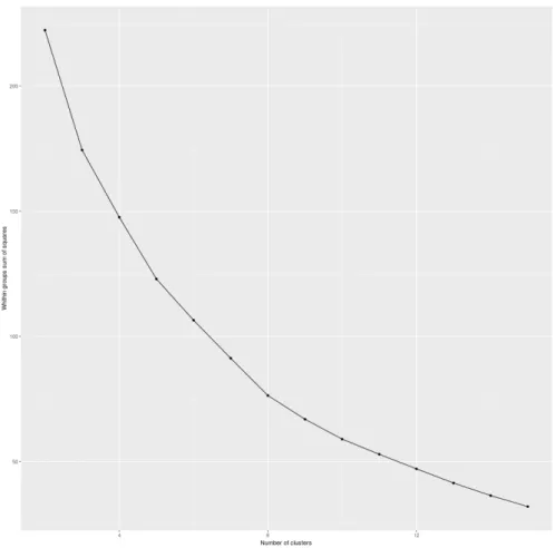
Firstly the number of optimal k cluster has to be selected. In order to ana-lyze the structure and pick a k suitable for every years, we evaluate the Weight Within Cluster (WSS) metric for the years which exhibit the higher absolute distance between the data. Year 2014 has been selected for this analysis.
Figure2shows the WSS of all the selected causes variables. It clearly shows
that there is no cluster number which is considerable better then the previous one, thus no elbow point is clearly visible. This suggests us that the input data are quite heterogeneous in high dimension space and we could select k =2 as suggested by the distance figures.
Figure 2: WSS of K-Means clustering on year 2014.
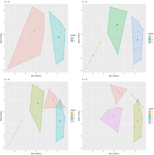
In addition we could graphically evaluate the different cluster for different values of k. Figure3shows the clusters derived with values of k ranging from
Figure 3: WSS of K-Means clustering on year 2014.
Figure 4, 5 shows same results for years 2016 and 2002. Here we could
observe that with k >2, k-means algorithm introduces non desiderable arti-facts.
Figure 5: WSS of K-Means clustering on year 2002.
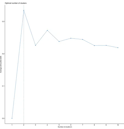
Thus we opted for a value of 2, this is further observable from Figure 6,
where the average silhouette width for each number of cluster is computed. In the following section we present the procedure in order to estimate the op-timal k value, but for this let’s stick to this value. This results in the clustering structure presented in Table ??.
Figure 6: K-Means average silhouette width for year 2014.
Figure 7shows the derived cluster analysis on years 2004, 2008, 2012 and
Figure 7: K-Means cluster analysis for years 2004, 2008, 2012 and 2016.
TODO: Show here dimensions which end up in PCA1 and PCA2. Table 7presents the clustering analysis for the all time period.
T2002 T2003 T2004 T2005 T2006 T2007 T2008 T2009 T2010 T2011 T2012 T2013 T2014 T2015 T2016 AUS 1 1 2 1 2 2 2 1 1 1 2 1 2 2 AUT 2 1 2 2 2 1 1 1 2 1 2 2 2 BEL 1 2 1 2 1 1 2 1 1 1 2 1 2 2 2 CAN 1 1 2 1 2 2 2 1 1 1 2 1 2 2 2 CZE 2 2 1 2 1 1 1 2 2 2 1 2 1 1 1 DNK 1 1 2 1 2 2 2 1 1 1 2 1 2 2 2 FIN 1 2 1 2 2 2 1 1 1 2 1 2 2 2 FRA 2 1 2 1 1 2 1 1 1 1 1 1 1 1 DEU 1 2 2 2 1 1 1 2 1 2 2 2 GRC 2 2 1 2 1 1 1 2 2 2 1 2 1 1 1 JPN 1 2 2 2 1 1 1 2 1 2 HUN 2 2 1 2 1 1 1 2 2 2 1 2 1 1 1 IRL 1 1 2 1 2 2 2 1 1 1 2 1 2 2 ITA 2 1 2 1 1 1 2 2 2 1 2 1 1 1 LVA 2 2 1 2 1 1 1 2 2 2 1 2 1 1 1 LTU LUX 1 2 2 2 1 1 1 2 1 2 2 MLT NLD 1 1 2 1 2 2 2 1 1 1 2 1 2 2 2 POL 2 2 1 2 1 1 1 2 2 2 1 2 1 1 1 PRT 2 2 1 2 1 1 1 2 2 2 1 2 1 1 1 ROU SVK 2 2 1 2 1 1 1 2 2 2 1 2 1 1 1 SVN 2 1 2 1 1 1 2 2 2 1 2 1 1 1 ESP 1 1 1 2 1 1 1 2 2 2 1 2 1 1 1 SWE 1 1 2 1 2 2 2 1 1 1 2 1 2 2 2 GBR 1 1 2 1 2 2 2 1 1 1 2 1 2 2 2 NOR 1 2 2 2 1 1 1 2 1 2 2 2 NZL 2 2 2 CHE 1 2 2 2 1 TUR 1 2 2 2 2 1 1 1 USA 1 1 2 1 2 2 2 1 1 1 2 1 2 2 2 WSS 128.946 152.154 168.933 212.401 210.949 215.681 235.818 228.930 219.978 217.488 200.970 209.983 222.270 214.604 193.234
Table 7: K-Means clustering results over the entire period.
Since cluster labels are not stable for a given country, it is interesting to observe the country which are clustered together for multiple years, in par-ticular the countries which have the same pattern trough time. Figure 8
vi-sualizes these information by evaluating the distance between the pattern followed by each country, thus a null distance means that that countries have been clustered together for the entire time span, whereas a non null distance measures the different evolution in the clustering groups.
Figure 8: K-Means cluster pattern analysis for the entire period.
Groups revealed thus are:
1. GRC, SVK, PRT, POL, LVA, HUN, CZE, TUR*, ITA*, SVN*, ESP (2002, 2003), FRA(2008, 2009, 2010, 2011, 2013)
2. AUS, AUT, BEL, CAN, DNK, FIN*, DEU, USA, GBR, SWE, NLD, JPN*, IRL, LUX*, NOR*, CHE*
Where (*) means that the series have some missing data, whereas i means that the country differs from that pattern for the i year.
4.1.3 Partition Around Medoids
Partition around medoids (PAM) originally proposed by Kaufman and Rousseeuw [35], is a clustering algorithms which maps a distance matrix into a specified
number of clusters, thus the algorithm tends to cluster together points with similar dissimilarity matrix, using a generic distance function. This, in partic-ular, is one of the key properties of PAM, the ability to perform its procedures with any specific distance function or matrix.
In addition the notion of the silhouette function and the averages per clus-ter, proposes a robust approach in order to evaluate the quality of the cluster
itself. Trough this work we have used the cluster package.
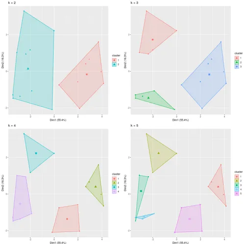
As with the k-means approach we would like to estimate the best number of cluster for our data set, thus Figure9 shows the average silhouette width
as a function of the number of medoids for years 2016, 2012, 2008 and 2004.
Figure 9: Average Silhouette Width as a function of medoids.
This shows the a two cluster choice would be optimal for the entire period. Figure10shows the silhouette width for each country into the two medoids
for the same analyzed years. An high values of solhouette width means that the country is well matched against its cluster, whereas a close to 0 value means that it is poorly matched against its cluster.
Figure 10: Silohuette width for each country.
As for k-means procedure, Figure ?? shows the distribution of clusters against the first two principal components for years 2016, 2012, 2008 and 2004.
Figure 11: Cluster representation over principal components.
TODO
T2002 T2003 T2004 T2005 T2006 T2007 T2008 T2009 T2010 T2011 T2012 T2013 T2014 T2015 T2016 AUS 1 1 1 1 1 1 1 1 1 1 1 1 1 1 AUT 1 1 1 1 1 1 1 1 1 1 1 1 1 BEL 1 2 1 1 2 1 1 1 1 1 1 1 1 1 1 CAN 1 1 1 1 1 1 1 1 1 1 1 1 1 1 1 CZE 2 2 2 2 2 2 2 2 2 2 2 2 2 2 2 DNK 1 1 1 1 1 1 1 1 1 1 1 1 1 1 1 FIN 1 1 1 1 1 1 1 1 1 1 1 1 1 1 FRA 1 1 2 1 1 1 1 1 2 2 2 2 2 2 DEU 1 1 1 1 1 1 1 1 1 1 1 1 GRC 2 2 2 2 2 2 2 2 2 2 2 2 2 2 2 JPN 1 1 1 1 1 1 1 1 1 1 HUN 2 2 2 2 2 2 2 2 2 2 2 2 2 2 2 IRL 1 1 1 1 1 1 1 1 1 1 1 1 1 1 ITA 2 2 2 2 2 2 2 2 2 2 2 2 2 2 LVA 2 2 2 2 2 2 2 2 2 2 2 2 2 2 2 LTU LUX 1 1 1 1 1 1 1 1 1 1 1 MLT NLD 1 1 1 1 1 1 1 1 1 1 1 1 1 1 1 POL 2 2 2 2 2 2 2 2 2 2 2 2 2 2 2 PRT 2 2 2 2 2 2 2 2 2 2 2 2 2 2 2 ROU SVK 2 2 2 2 2 2 2 2 2 2 2 2 2 2 2 SVN 2 2 2 2 2 2 2 2 2 2 2 2 2 2 ESP 1 1 1 2 2 2 2 2 2 2 2 2 2 2 2 SWE 1 1 1 1 1 1 1 1 1 1 1 1 1 1 1 GBR 1 1 1 1 1 1 1 1 1 1 1 1 1 1 1 NOR 1 1 1 1 1 1 1 1 1 1 1 1 NZL 1 1 1 CHE 1 1 1 1 1 TUR 2 2 2 2 2 2 2 2 USA 1 1 1 1 1 1 1 1 1 1 1 1 1 1 1 Sil 0.413 0.362 0.389 0.386 0.383 0.388 0.383 0.395 0.399 0.386 0.403 0.411 0.410 0.412 0.393
Table 8: PAM clustering results over the entire period.
Figure 12: PAM cluster pattern analysis for the entire period.
4.2 d ata r e d u c t i o n
4.2.1 Dimension Reduction
Broadly viewed, dimension reduction has always been a central statistical concept. In the second half of the nineteenth century, reduction of observations was widely recognized as a core goal of statistical methodology, and princi-pal components (PCs) were emerging as a general method for the reduction of multivariate observations [1].
Given a response variable y and a p-dimensional predictor vector x, a di-mension reduction is a function R : Rp → Rq, q< p that maps x to a subset of Rqwhich would like to explain y, thereby reducing the dimension of x.
A dimension reduction R(x) is said to be sufficient if at least one of the following three statements holds [9] [1]:
• inverse reduction, x|(y, R(x)) ∼x|R(x)
• forward reduction, y|R(x) ∼y|x • joint reduction, y⊥ x|R(x)