Calibration of biochemical network models

Calibration of biochemical network models

The Microsoft Research - University of Trento Centre for Computational and Systems Biology

lecca@cosbi.eu Alida Palmisano

The Microsoft Research - University of Trento Centre for Computational and Systems Biology

DISI - University of Trento palmisano@cosbi.eu

Corrado Priami

The Microsoft Research - University of Trento Centre for Computational and Systems Biology

DISI - University of Trento priami@cosbi.eu

Guido Sanguinetti

Dept. of Computer Science - University of Sheffield, UK G.Sanguinetti@dcs.shef.ac.uk

Calibration of biochemical network models

Paola Lecca 1_{, Alida Palmisano} 1_{, Corrado Priami} 1 _{and Guido Sanguinetti} 2_, 1 _{The Microsoft Research – University of Trento}

Center for Computational and Systems Biology, Trento, Italy E-mail: {lecca, palmisano, priami}@cosbi.eu

2 _{Dept. of Computer Science, University of Sheffield, Sheffield UK}

E-mail: G.Sanguinetti@dcs.shef.ac.uk

Abstract

The estimation of parameter values (model calibration) is the bottleneck of the computational analysis of biological systems. Modeling approaches are central in systems biology, as they provide a rational framework to guide systematic strategies for key issues in medicine as well as the pharmaceutical and biotechnological industries. Inter- and intra-cellular processes require dynamic models, that contain the rate constants of the biochemical reactions. These kinetic parameters are often not accessible directly through experiments. Therefore methods that estimate rate constants with the maximum precision and accuracy are needed.

We present here a new method for estimating rate coefficients from noisy observations of concentration levels at discrete time points. This is traditionally done by computing the least-squares estimator. However, estimation of the error function generally requires solving the reaction rate equations, which can become computationally unfeasible. We propose an alternative approach based on a probabilistic, generative model of the variations in reactant concentration. Our method returns the rate coefficients, the level of noise and an error range on the estimates of rate constants. Its probabilistic formulation is key to a principled handling of the noise inherent in biological data, and it allows for a number of further extensions. The mathematical procedure presented here has been implemented in a software tool, named KInfer.

1 Background

The relation between the instantaneous rate of reaction and the concentrations of the reactants at any moment is given by the law of mass action: i.e. the rate at which a substance takes part in a reaction is proportional to its concentration raised to a power which represents the number of molecules taking part in the reaction. Such formulation is made for simultaneous as well as isolated reactions, and for heterogeneous as well as homogeneous systems. The ability to infer these constants of proportionality for a system of biochemical reactions is crucial in systems biology, yet their direct measurement is a challenging experimental problem. Parameter estimation is commonly achieved by the best fit of numerical simulations to experimental observations. The fitting procedure is based on optimization techniques where a measure of the distance between model prediction and experimental data (the cost function) is used as the optimality criterion to be minimized. In most approaches dealing with parameter estimation the cost function is the likelihood function,

also know as joint transitional density. It expresses the probability of obtaining the observed outcomes in terms of measured systems variables and parameters. Thus it can be used to determine unknown parameters based on known outcomes. The optimal values of the parameters can be estimated by maximizing the likelihood function (maximun likelihood criterion) or, equivalently, by minimizing the log-likelihood function. However, when estimating parameters of dynamical systems with optimization methods a number of difficulties may arise, the main of which are convergence to local solutions, very flat objective function in the neighborhood of the solution, over-determined models, and non-differentiable terms in the systems dynamics. Due to the non-linear nature of the dynamics of the biological processes, these problems are often multimodal, so that traditional gradient based methods fail to identify the global solution and may converge to a local minimum. Moreover, in the case in which a bad fit has been performed, there is no way of knowing if it is due to a wrong model structure or if it is consequent to a local convergence.

The recent literature reports many examples of new effective methods attempting either to work out these difficulties or to develop new methodologies of parameter estimation both in deterministic and stochastic models. Here we briefly mention the most recent ones. Polisetty et al. in [13] suggested global optimization techniques as alternative to traditional local methods. Rodrigez-Fernandez et al. in [15] developed a hybrid stochastic-deterministic global optimization method. Moles et al. in [12] explored several state-of-the-art deterministic and stochastic global optimization techniques and compared their accuracy and effectiveness on nonlinear biochemical dynamic models. Tian et al. [7] presented simulated maximum likelihood method to evaluate parameters in stochastic models described by stochastic differtial equation. They propose different types of transitional probability and a genetic optimization algorithm to search for optimal reaction rates. Chou et al. [4] developed an alternate regression method, that dissects the parameter inference problem into iterative steps of linear regression. Sugimoto et al. [16] provided a computational technique based on genetic programming that simultaneously generates biochemical equations and their parameters from time series data. Reinker et al. [14] are the authors of the approximate maximum likelihood method and the singular value decomposition likelihood method that estimate stochastic reaction constants from molecule count data measured with errors at discrete time points. Tools for parameter fitting through regression or maximum likelihood methods can be found as integral part of simulation tools (e. g. Copasi [10]), but there exist also ―stand-alone‖ software exclusively designed for that purpose, like Splindid [2] and PET [21]. Finally we mention the works of Boys [3], Golitki [8] and Wilkinson [19, 20], that developed Bayesian model-based inference techniques. Baysesian scheme depart from the approaches previously mentioned. They offer some advantages over the maximum likelihood methods, for instance when the volume of data is limited or the analytic form of the kinetic model makes the maximization of the likelihood not straightforward. The disadvantages of the most part of the current tools for paramter estimation is the lack of robustness to the noise and the absence of any estimates of experimental error in their outcome. Experimental uncertainties on parameters propagate from the measurements of the concentrations of the species. Returning the parameters with an estimate of their uncertainty is essential if we want to use the tool in the context of optimal experimental design. Moreover, the most part of the current tools, based on optimization techniques suffer from the problem of univocally finding the solution global optimization, and ask the user to provide a priori to the optimization algorithm the region of parameter space in which to perform the search for the global maxmimum.

In this paper we present a novel approach to the model calibration, that proposes the solution to these difficulties. The method is based on a probabilistic, generative model of the variations in reactant concentration. Given reactant species, we observe time series concentrations for each of the species, gathered in state vectors , our method discretizes the law of mass action and provides a tool to predict the values of the variables at time , conditioned on their values at the previous time point. The

variations of the concentration of the species at different time points are conditionally independent by the Markov nature of the discrete model of the law of mass action. Assuming the observation noise to be Gaussian with variance , the probability of observing a variation for the concentration of species between time and is a Gaussian with variance depending on and mean the expectation value of the law of mass action under the noise distribution. The discretization of the law of mass action provides a model for the variations of the species concentration, rather than a model for the time-trajectory of the species concentrations. This makes the evaluation of the expectation value of law mass action function (the integral of the transitional probability) simpler and analytically tractable. The rate coefficients and the level of noise are then obtained by maximizing the likelihood function defined by the observed variations. Our method returns the rate coefficients, the level of noise and an error range on the estimates of rate constants. Its probabilistic formulation is key to a principled handling of the noise inherent in biological data, and it allows for a number of further extensions, such as a fully Bayesian treatment of the parameter inference and automated model selection strategies based on the comparison between marginal likelihoods of different models. Finally, the implementation of this method may be used as an interface tool, connecting the outcomes of the wet-lab activity for the concentration measurements and the software for the simulation of chemical kinetics.

We show the ability of our algorithm of obtaining reasonable estimates for the rate coefficients in case studies of different complexity including first and second order chemical reactions, didactical examples of biochemical networks, and more complex biological pathways. In particular we present the results of the application of our inference procedure to the following case studies: the gene transcription, the gene transcription regulation, the gene expression, the thermal isomerization of -pinene, the fermentation pathway in Saccharomyces Cerevisiae and finally the activation of M-phase promoting factor in the cell cycle. The parameters of the kinetics of these pathways are known, since they were experimentally determined and widely documented in literature. Thus, we could compare our estimates of the parameters with the known values to assess the soundness of the methodology and the performance of its implementation.

The technical report is divided into four sections: the next section describes the inference model. Section 3 illustrates the results of the method applied to the case studies. Finally Section 4 points out some conclusion and future directions. The work is mainly focused on the mathematical foundations of the inference method and reports some preliminary results obtained with KInfer, the software prototype implementing the procedure. The method of inference, proposed here, returns estimates of the rate coefficients with their experimental uncertainty, and since none of the considered tools returns the experimental error of the outputs (rather most of them consider standard deviation on the average values of the rate constant obtained by several algorithm runs), here we test the method by evaluating the discrepancy of our estimates from the expected values. The comparison of Kinfer with other tools in term of performances will be considered as future work, as the performance analysis have to be based on a common definition of error and accuracy, that, at the moment of writing, is under investigation. In each case study we refer the reader to the suitable literature references.

2 The model

Consider reactant species, with concentrations , that evolve according to a

system of rate equations

where , , is the vector of the rate coefficients, which are present in the expression of the function . We wish to estimate the set of parameters ( ), whose element is the set of rate coefficients appearing in the rate equations of i-th species, therefore

.

is the vector of concentrations of chemicals that are present in the expression of the function for the species .

According to the law of mass action, the functions have the general form

. (2.2)

In this equation , with , , is a vector whose set of elements is a subset of

the set of elements of the vector .

The function is the product of reactant concentrations, accordingly to the empirical law of rate equation as follows

where denotes the partial order of reaction with respect to the reactant having concentration Substituting these expressions in Eq. (2.2) gives

(2.3)

We assume we have noisy observations at times , where is a Gaussian

noise term with mean zero and variance . We also assume a number of concentration measurements for each considered species.

We discretize the rate equation (1.1) as a finite difference equation between the observation times,

where . In Eq. (1.4) the rate equation is viewed as a model of increments/decrements of reactant concentrations; i.e., given a value of the variables at time , the model can be used to predict the value at the next time point. Increments/decrements between different time points are conditionally independent by the Markov nature of the model (2.4). Therefore, given the Gaussian model for the noise, it is possible to estimate the probability to observe the value given the model at time , and the set of parameters

, as

(2.5) Moreover, by symmetry, the true value of is normally distributed around the observed value , so that

(2.6) Therefore, the probability to observe a variation for the concentration of the i-th species between the time

and , given the parameter vector is

(2.7) and

(2.8) where is the number of chemical species in the expression for .

While the increments/decrements are conditionally independent given the starting point , the random variables are not independent of each other. Intuitively, if happens to be below its expected value because of random fluctuations, then the following increment can be expected to be bigger as a result, while the previous one will be smaller. A simple calculation allows us to obtain the covariance matrix of the vector of increments for the i-th species.

This is a banded matrix with diagonal elements given by

and a non-zero band above and below the diagonal given by

with all other entries zero. The likelihood for the observed increments/decrements therefore will be

(2.9) where

and

The Eq. (2.9) can be optimized w. r. t. the parameters of the model to yield estimates of the parameters themselves and of the noise level.

The chief numerical problem of this approach is the computation of the expectations of the rate functions given by equation (2.8). Non-integer values of the coefficients can make estimating the integral analytically difficult. We propose an approximate method in which the Gaussian noise is replaced by an approximate uniform (white) noise, with the amplitude of the uniform noise being obtained as a sample from the Gaussian cumulative distribution function.

At the first order, for small we can approximate the Gaussian with zero mean and variance $\sigma$ with an uniform distribution defined on the interval , so that

(2.10) where Therefore (2.11) Now, since we have

(2.12) where S is the set containing the indexes referring to all the species appearing in .

If in the Eq. (2.9), is substituted with the expression (2.12) , Eq. (2.9) becomes more tractable can be optimized w. r. t. the parameters and . The values of the model’s parameter for which

has a maximum are the most likely values giving the observed kinetics.

2.1 Initial guesses and bounds for the parameter values

The search for the optimal values of rate constants can be made more efficient if we provide the algorithm of optimization of Eq. (2.9) with the initial guesses for these constants. In this way the algorithm does not waste time in exploring large regions of the parameter space or regions in which the model (2.4) is not valid. Our model calibration method also includes a procedure for the automatic calculation of the initial guesses of the parameters. Therefore, the task to direct the inference method to efficiently exploring the parameter space is not left to the user, that often does not have a precise idea about a reasonable value of the parameters. The method of calculating the approximated guesses of the parameter is explained in the following.

The rate equation of a species , ( ), is a measure of the slope of the curve of the function as follows

. (2.1.1)

We obtained the slopes in each time point , ( ), from the experimental data by using the Stineman algorithm. This algorithm provides a procedure of interpolation and returns the slope of the interpolating function running through a set of points in the xy-plane. The functions are the same as in Eq.

(2.2). The left-hand side of the equations of system (2.1.1) is determined by the Stineman algorithm, whereas the right-hand side is an expression containing the unknown parameters . In general the system (2.1.1) has

equations and at most unknown rate constants. Since in general , where is the cardinality of , the system could be singular. In those cases, we considered a different time re-sampling of the Stineman curve interpolating the experimental data. The new set of time-points are those in which the values of the interpolating curve have null slope. In this way the curve is under-sampled and the system has a less number of equations. If the system is still singular, the number of equations is cut down further on, until the equality is satisfied, and thus the system can be solved to find the approximated values of unknown parameters to be used as initial guesses for the algorithm of optimization. Determining the parameter values with the maximum likelihood of being correct is only part of the parameter estimation problem. It is equally important to find a realistic measure of the precision of those parameters. Since the experimental values of the concentrations are affected by errors, then we considered the propagation of these errors to the estimate of the parameters.

A system of equations similar to the system (2.1.1) can be written also for the errors affecting the slopes :

(2.1.2) where, using (2.3), we obtain

(2.1.3)

For convenience, consider a single term of the sum on the right-hand side of Eq. (2.1.3), for instance the first, and calculate the relative error on this term as follows

(2.1.4)

where is the cardinality of the set . Therefore, Eq. (2.1.3) becomes

(2.1.5)

Assuming that the measurements of times are not affected by errors, the error is calculated from Eq. (2.4) as follows

(2.1.6) where is the experimental error on the measurement of concentration of species i at time . In Eq. (2.1.6) the left-hand side is determined from the data. The right-hand side contains the unknown parameters

, that are the errors on the estimates of the rate constants. They are calculated by solving the system of equations of the form of Eq. (2.1.5) for all the involved species with the same criteria we used to make solvable the system (2.1.1).

The optimization algorithm for the function (2.9) is provided with the initial guesses of the parameters and their bounds obtained as solutions of system (2.1.1) and system (2.1.2), respectively. Therefore, without any intervention by the user, the search for the maxima of the probability density function of the observed concentration increments/decrements is addressed to the region of parameter space in which the empirical model (2.4) holds for the observed data.

3 The structure of KInfer

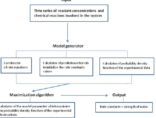
We developed the prototype KInfer that implements the procedure described in the previous section. The tool consists of four main blocks: 1) the input interface, 2) the model generator, 3) the maximization algorithm and 4) the output interface (Fig. 1).

Figure 1: Scheme of KInfer's design.

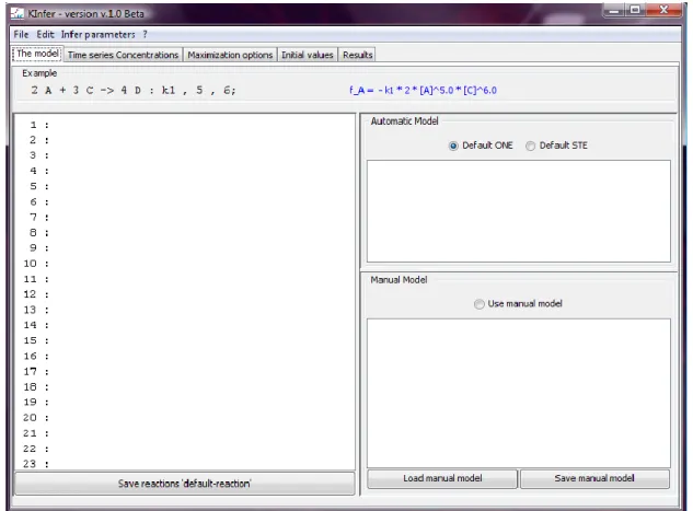
A screenshot of the front-end is shown in Fig. 2. The tool takes as input the set of chemical reactions describing the kinetics of the systems, specified in the following syntax.

On the left-hand side of the arrow, the reactants ( ) and the reactants stoichiometric coefficients ( ) are indicated, whereas on the right-hand side the products ( ) and the product

stoichiometric coefficients ( ) are indicated. The reaction specification contains also the indication of the name of the rate constant after colon and the partial orders of reaction ( ). The specification of the reactions must end with semicolon. Along with the specification of the set of reactions involved in the system, KInfer requires the experimental time series data, in tabular text format, of the concentration (or number of molecules) of the species present in the system. The option ―Load concentrations…‖ in the File menu of the front-end allows the user to download the experimental times series of concentrations.

From the set of chemical reactions the tool automatically generates the ordinary differential equations model, consisting of a system of equations of the form of Eq. (2.3) (See the field ―Automatic model‖ in the front-end in Fig. 2). However, the user is allowed to insert a different model that can be entered in the ―Manual Model‖ part of the interface (Fig. 2). The user is allowed also to enter an ordinary differential equation model without specifying the reaction in the standard ―chemical‖ notation.

Figure 2: front-end of KInfer.

The tool processes the inputs and it derives from the data set of the concentration time-series and from the model of rate equation the form of the probability density function (2.9) to maximize and the initial guesses for the parameters. Although the tool automatically calculate the initial guesses of the parameters, the user is allowed to change the estimated values as well as to directly insert new different estimates.

Our choice of the optimization algorithm has been driven by the fact that a biological model of realistic size and complexity presents a high number of parameters with possible nonlinear relations between them. In such cases the use of methods belonging to the class of Genetic Algorithms (GA) [22] is recommendable. A genetic algorithm is a population based stochastic optimization technique, that, starting from a set of initial guesses about the solution, determines the next set of possible solutions to the optimization problem on the basis of the results obtained from the preceding set. These methods have been designed primarily to address problems that

cannot be tackled through traditional optimization algorithms. Such problems are characterized by discontinuities, lack of derivative information, noisy function values and disjoint search spaces. In the GA approach, the evolution starts from a population of randomly generated individuals. Then in each generation the fitness of every individual in the population is evaluated and multiple individuals are stochastically selected from the current population (based on their fitness). The chosen individuals are modified (recombined and possibly randomly mutated) to form a new population. The new population will be used in the next iteration of the algorithm. The algorithm terminates when either a maximum number of generations has been produced, or a satisfactory fitness level has been reached for the population.

The selection operation involves the evaluation of each possible solution with respect to the target assigned: the lower the log-likelihood value is, the better the solution is considered. The next step is to select the solutions for the next generation in such a way that those with higher fitness have higher probability of selection: to each guessed solution will be assigned a selection probability derived by the ratio of its square fitness and the sum of the squared fitness of all the solutions. The selected solutions are then subjected to cross-over, mutation and innovation operators. To realize cross-over, every two parents create two children in the following way: the algorithm selects randomly from the first parent how many and which variables will have to be kept in the first child. Then from the second parent the algorithm takes the complementary number of variables and uses these values to complete the first child. The second child is then built with the remaining variables of the two parents. The mutation operation, with a low probability (in our examples p = 0.1), randomly selects one variable to be mutated. After the selection, the value of the variable is changed selecting (again randomly) from the possible values it can take excluding the currently one. Finally, the innovation operator randomly select new solutions never tested to be performed. Usually this operator is kept at low rate (here at 5%), trying to optimize the trade-off between exploration and exploitation. Once the new population of experiments is derived from the algorithm it is then proposed as a new generation for the next algorithm iteration. The size of each population of solution in each generation is maintained constant.

4 Case studies

Here we provide some validation tests on biochemical networks. For each case study we briefly describe the topology of the reaction network, and we report our estimates of the kinetic rate constants compared with the estimates obtained by other studies and approaches. We did not include in the text of this manuscript the experimental and/or synthetic time series of the concentrations we used as input of our procedure to infer the parameter. They are separately provided as additional files.

We also show the model simulations obtained with the estimated parameters and with the actual parameters, in order to show the discrepancy between the actual expected time behavior and the estimated time behavior due to the propagation of the errors on rate constants to the time course of the concentration.

The errors on the parameter estimates computed by our procedure are not computational errors imputable to the precision of the integration algorithms and the optimization algorithm. They are experimental errors that we expect to obtain from input data affected by and/or simulated with experimental errors. Moreover they depend on the time resolution at which the concentration measurement is recorded. Therefore, their values are not comparable with the values of errors on the parameters estimates obtained by the references cited in each case study, to which we refer the reader for a more detailed discussion on the computation of the estimates precision, accuracy and errors.

The results we present in the next section confirm that the procedure converges to the expected solution within the experimental errors and the strength of noise affecting the input data.

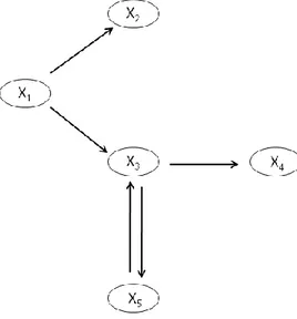
4.1 Didactic example: a small biochemical network

The system depicted in Figure 3 is representative of a small biochemical network of 4 interacting species. The network has two feedback loops: 1. the species X5 inhibits the production of species X1, and 2. The species X4

promotes the activation of X5.

Figure 3: A didactic example of biochemical network with four variables [4, 16].

A numerical implementation with typical parameters is

This system of equation is used to create the artificial time series data of the five involved variable. Typical units might mM for the concentration and minutes for the times, but the example could as well run on an hourly scale and with variables of different nature. Table 1 lists the results. Within the experimental uncertainties, these results are in agreement with those in [4].

Actual rate constants Bounds for the initial guesses Estimated rate constants

1 12 [10.18; 13.84] 11.37 ± 3.66 2 10 [8.28; 11.74] 9.39 ± 3.46 3 8 [9.81; 9.87] 9.83 ± 0.06 4 3 [3.92; 3.99] 3.98 ± 0.07 5 3 [2.91; 2.96] 2.94 ± 0.05 6 5 [4.89; 4.91] 4.90 ± 0.02 7 2 [1.50; 2.55] 1.84 ± 1.05 8 6 [4.01; 8.17] 5.5 ± 4.16

Estimated noise strength = 0.3

4.2 Gene transcription

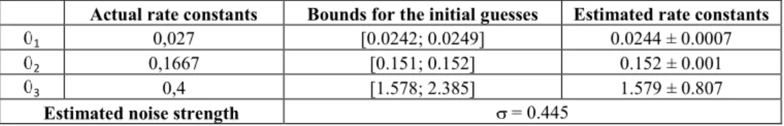
In this test, we consider the transcription of a single gene as given by the model of Golding et al. in [7, 14]. The DNA for the tagged mRNA is switched on and off by polymerase binding and unbinding, respectively. Only polymerase-bound DNA is transcribed into mRNA. The system is depicted in Figure 5. The reaction rates associated with the reaction R1: DNAOFF → DNAON, R2: DNAON → DNAOFF, and R3: DNAON →

DNAON + mRNA are , . and , respectively. As initial

conditions in this system, we set DNAOFF =1, DNAON = 0 and mRNA = 0.

Figure 4: Golding model of gene transcription process.

Our estimates in Table 2 are in strong agreement with the actual ones as well as with those obtained by Reinker et al. [13].

Actual rate constants Bounds for the initial guesses Estimated rate constants

1 0,027 [0.0242; 0.0249] 0.0244 ± 0.0007

2 0,1667 [0.151; 0.152] 0.152 ± 0.001

3 0,4 [1.578; 2.385] 1.579 ± 0.807

Estimated noise strength = 0.445

Table 2: Estimates of the kinetic parameters of the Golding’s model of gene expression.

4.3 Transcriptional regulation

Figure 7 illustrates a model of transcriptional regulation that was proposed by Goutsias [9] and reported in [14]. Here, the mRNA is translated into a protein monomer M that can dimerise. The dimer D, in turn, can bind to its DNA and acts as a transcription factor to auto-regulate its own mRNA production. Both mRNA and protein are degraded at constant rates. The set of reactions of this network is the following

As in [14], we used this set of reactions to generate, with the Dizzy simulator [24], a database of deterministic time series of number of molecules for each component in the system. As initial values we used M = 2, D = 4, DNA = 2, and mRNA = 0, DNA∙D = 0. All the reaction constants are in units of per seconds.

Figure 7: Goutsias transcriptional regulation system.

Table 3 reports the estimates of the rate constants in agreement with the actual values and with the results in [9].

Actual rate constants Bounds for the initial guesses Estimated rate constants

1 0,043 [1.3750; 1.3784] 1.3769 ± 0.0034 2 0,0007 [3.3416; 3.3811] 3.3499 ± 0.0396 3 0,715 [0.0859; 0.1203] 0.1051 ± 0.0344 4 0,00395 [0.00340; 0.00386] 0.003777 ± 0.000459 5 0,02 [0.0468; 0.1157] 0.1118 ± 0.0688 6 0,4791 [1.3057; 1.4794] 1.4682 ± 0.1737 7 0,083 [0.1928; 0.1978] 0.1973 ± 0.0051 8 0,5 [0.0801; 0.1898] 0.112 ± 0.1097

Estimated noise strength = 0.2998

4.4 Gene expression

Figure 9 illustrates the gene expression of a single gene with both transcription and translation. The model consists in the following set of reactions: R1: DNA → DNA + mRNA, R2: mRNA → () , R3: mRNA +

protein, and R4: protein → (). The kinetic constants associated to these reactions are: ,

, , and ([16]). The results of our inference

procedure are listed in Table 5.

Figure 9: Gene expression of a single gene.

Table 4: Estimates of kinetic rate constants of the model of gene expression in Figure 9.

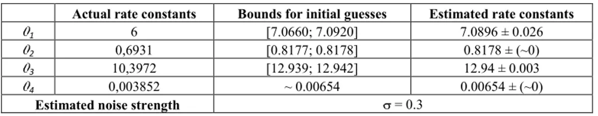
4.5 Isomerization of -pinene

In this case study we estimate the rate constants of a complex biochemical network describing the thermal isomerization of -pinene (X1) to dipentene (X2) and allo-ocimen (X3) which in turn yields - and -pyronene

(X4) and dimer (X5). This process is described by the reaction scheme reported in Figure 11 and investigated

in [5, 15]:

Actual rate constants Bounds for initial guesses Estimated rate constants

1 6 [7.0660; 7.0920] 7.0896 ± 0.026

2 0,6931 [0.8177; 0.8178] 0.8178 ± (~0)

3 10,3972 [12.939; 12.942] 12.94 ± 0.003

4 0,003852 ~ 0.00654 0.00654 ± (~0)

The best known solution for the kinetics are , ,

, , and [15].

Figure 11: Reaction scheme for the thermal isomerization of -pinene (X1).

The deterministic model of the network is the following:

It has been used to generate the database of the time series of concentration used as artificial input to KInfer. Table 5 reports the estimates for these rate constants obtained by our procedure and Figure 10 shows the expected and the estimated time course of the species concentrations. High discrepancy are obtained for the time course of and , reflecting the inaccuracy in the estimate of and .

Actual rates Bounds for the initial guesses Estimated rate constants

1 5,95E-05 [5.63; 6.11]×10E-5 (5.86 ± 0.05) × 10E-5

2 2,96E-05 [2.4; 3.0]×10E-5 (2.8 ± 0.6) ×10E-5

3 2,05E-05 [0; 0.006] (6.19 ± 76.4) ×10E-5

4 2,75E-04 [3.78; 4.54] ]×10E-4 (4.16 ± 0.08) × 10E-4

5 4,00E-05 [10.3; 12.0] ×10E-5 (11.1 ± 0.2) × 10E-5

Estimated noise strength = 0.745

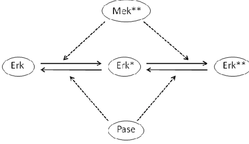
4.6 MAP-Kinase cascade

Figure 13 depicts the last step of the mitogen-activated protein kinase (MAPK) cascade. Activated MPAK kinase (Mek**) catalyzes the activation of MAPK (Erk) by phosphorilation, resulting in the activated form Erki**. The deactivation of the active form is catalyzed by the phosphatase (Pase). The picture shows 12 reactions as follows:

R1: Erk + Mek** → Erk ∙ Mek**;

R2: Erk ∙ Mek** → Erk + Mek**;

R3: Erk ∙ Mek** → Erk* + Mek**;

R4: Erk* + Mek** → Erk* ∙ Mek**;

R5: Erk* ∙ Mek** → Erk* + Mek**;

R6: Erk* ∙ Mek** → Erk** + Mek**;

R7: Erk** + Pase → Erk** ∙ Pase;

R8: Erk** ∙ Pase → Erk** + Pase;

R9: Erk** ∙ Pase → Erk* + Pase;

R10: Erk* + Pase → Erk* ∙ Pase;

R11: Erk* ∙ Pase → Erk* + Pase;

R12: Erk* ∙ Pase → Erk + Pase.

The kinetic rates associated to these reactions have been chosen, accordingly to Faller et al. [23] as follows:

.

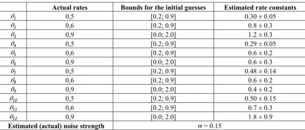
With the following initial values for nano-molar concentrations [Erk] = 15, [Pase] = 5, [Erk*] = 5, [Erk**] = 5, [Mek**] = 15; [Erk ∙ Mek**] = 5, [Erk* ∙ Mek**]=5; [Erk* ∙ Pase] = 5, and [Erk** ∙ Pase] = 10, we generated the artificial data set of the time series of concentrations and used them as input for our parameter inference procedure. Table 6 shows the estimates of the parameters.

Actual rates Bounds for the initial guesses Estimated rate constants 1 0,5 [0.2; 0.9] 0.30 ± 0.05 2 0,6 [0.2; 0.9] 0.8 ± 0.3 3 0,9 [0.0; 2.0] 1.2 ± 0.3 4 0,5 [0.2; 0.9] 0.29 ± 0.05 5 0,6 [0.2; 0.9] 0.6 ± 0.2 6 0,9 [0.0; 2.0] 0.6 ± 0.3 7 0,5 [0.2; 0.9] 0.48 ± 0.14 8 0,6 [0.2; 0.9] 0.6 ± 0.2 9 0,9 [0.0; 2.0] 0.4 ± 0.2 10 0,5 [0.2; 0.9] 0.50 ± 0.15 11 0,6 [0.2; 0.9] 0.7 ± 0.3 12 0,9 [0.0; 2.0] 1.8 ± 0.9

Estimated (actual) noise strength = 0.15

Table 6: Estimates of the kinetic rate constants of the last step of MAPK cascade in Figure 13.

4.7 Fermentation pathway in Saccharomyces Cerevisiae

The metabolic pathway is given in Figure 15. The structural and numerical specifications of this model are based on kinetic experiments and biochemical analyses [6]. The mass action equation for this model adapted from [13]. The model has 5 dependent variables, 9 independent variables and 16 unknown rate constants. According to [13], the observed concentrations of (in units of mM) at steady state are:

X1 (GIn) – Internal glucose = 0.0346,

X2 (G6P) – Glucose-6-phosphate = 1.011

X3 (FDP) – Fructose-1,6-diphosphate = 9.1876

X4 (PEP) – Phosphoenolpyruvate = 0.0095

X5 (ATP) – Adenosine triphosphate = 1.1278.

The values of the independent variables (mM min-1_{) are:}

X6 Glucose uptake = 19.7

X7 Hexokinase = 68.5

X8 Phosphofructokinase = 0 31.7

X9 Glyceraldehyde.3-phosphate dehydrogenase = 49.9

X10 Pyruvate kinase = 3.440

X11 Polysaccharide production (glycogen + trehalose) = 14.31

X12 Glycerol production = 203

X13 ATPase = 25.1

Figure 15: Model of anaerobic fermentation of glucose to ethanol, glycerol, and polysaccharides in Saccharomyces Cerevisiae [13].

The mass action model of the pathways is given by the following equations adapted from [13] and has been use to generate a synthetic database of concentration time series.

Actual rate constant Bounds for the initial guesses Estimated rate constants 0,8122 [1.07; 1.24] 1.17 ± 0.17 2,8632 [4.009; 4.146] 4.059 ± 0.137 2,8632 [0.0; 1.37] 0.38 ± 1.37 0,5232 [0.0; 0.314] 0.042 ± 0.315 0,0009 [0.0; 0.059] 0.057 ± 0.06 0,5232 [0.0; 0.070] 0.056 ± 0.071 0,011 [0.0; 0.439] 0.29 ± 0.44 0,0473 [0.0; 20.60] 0.13 ± 20.61 0,022 [0.0; 0.10] 0.06 ± 0.102 0,0945 [0.0; 199.19] 78.23 ± 199.2 0,022 [0.0; 0.15] 0.0021 ± 0.1545 0,0945 [26.91; 36.60] 27.26 ± 9.69 2,8632 [0.0; 0.0046] 0.004 ± 0.0047 0,0009 [0.0; 0.063] 0.014 ± 0.064 0,5232 [0.0; 0.26] 0.00093 ± 0.2618 1 [0.055; 0.135] 0.096 ± 0.08

Estimated (actual) noise strength = 0.29

Table 7: Estimates of the kinetic rate constants for the fermentation pathway model in Figure 15.

5 Conclusions

In this article, we presented a novel method for the estimation of reaction parameters and noise strength from time series of molecules counts or concentrations observed with error. We have shown that our procedure converges to the expected solutions within the bounds of the experimental errors that propagates from concentration measurements to the kinetic rate constants. The results confirm that the validity of the procedure and the validity of the discretized model of generalized mass action law for the rate equation in most cases, even if some discrepancies can be due to this approximation in some cases. However, results not shown here, and currently under investigation are showing that increasing the size of the initial guess about the model parameter minimizes the disagreements. Moreover, some important features missing from the existing method for model parameter inference are present in our method. The first is the implementation of a procedure, which automates the computation of the initial guesses of the parameters. In this way, the user is not forced to insert any a priori knowledge about the system, that often is quite hard to find, and, at the same time, the method is equipped with a rigorous procedure referring only to the experimental concentration measurements to identify a region of the parameter space where the optimization of the probability density function takes place. The second feature is the implementation of the error propagation. The evaluation of the experimental errors of the rate constants estimates is particularly useful if the procedure of parameter inference is incorporated in projects of experimental design. The size of the errors on the kinetic constants is indicative of the optmimality of the experimetal setup. Thus, any procedure devoted to the reduction of this error is definitely part of a methodology aiming to optimize the design of the experimental configuration.

Bibliography

1. Almeida, J., & Voit, E. O. (2004). Decoupling dynamicsl systems for oathway identification from metabolic profiles. Bioinformatics , 20: 1670-1681.

2. Bashi, K., Forrest, A., & Ramanathan, M. (2005). SPLINDID: a semi-paramteric, moel-based method for obtaining transcription rates and gene regulation parameters from genomic and proteomic expression profiles. Bioinformatics , 21 (20), 3873-3879.

3. Boys, R. J., Wilkinson, D. J., & Kirkwood, T. B. (2008). Bayesian inference for a discretely observed stochastic kinetic model. Statistics and Computing, Springer Netherlands.

4. Chou, I.-C., Martens, H., & Voit, E. O. (2006). Parameter estimation in biochemical systems models with alternating regression. Theoretical Biology and Medical Modelling , 3, 25.

5. Fuguitt, R., & Hawkings, J. E. (1947). Rate of thermal isomeration of -pinene in th eliquid phase. JACS

, 69, 461.

6. Galazzo, J. L., & Bailey, J. E. (1990). Fermentation pathway kinetics and metabolic flux control in suspended and immobilized Saccharomyces Cerevisiae. Enzyme Microb. Technol , 12, 162-172.

7. Golding, I., Paulsson, & Zawilski, S. M. (2005). Real-time kinetics of gene activity in individual bacteria.

Cell , 123, 1025-1036.

8. Golightly, A., & Wilkinson, D. J. (2008). Bayesian inference for nonlinear multivariate diffusion models observed with error. Computational statistics and data analysis , 52 (3), 1674-1693.

9. Goutsias, J. (2006). A hidden Markov model for transcrptional regulation in single cellsl. IEEE/ACM

Trans. Comput. Biol. Bioinform. , 3, 57-71.

10. Hoops, S., Sahle, S., Gauges, R., Lee, C., Pahle, J., Simus, N., et al. (2006). COPASI — a COmplex PAthway SImulator. Bioinformatics , 22, 3067-3074.

11. Lecca, P., Sanguinetti, G., Palmisano, A., & Priami, C. (2007). A new method for inferring rate coefficients from experimental time-consecutive measurement of reactant concentrations. Inernational

Conference on Systems Biology. Long Beach.

12. Moles, G. C., Mendes, P., & Banga, J. R. (2003). Parameter estimation in biochemical pathways: a comparison of global optimization methods. Genome Res. (13), 2467-2474.

13. Polisetty, P. K., Voit, E. O., & Gatzke, E. P. (2006). Identification of metabolic system paramters using global optimization methods. Theoreteical Biology and Medical Modelling , 3 (4).

14. Reinker, S., Altman, R. M., & Timmer, J. (2006). Parameter estimation in stochastic biochemical reactions. 153 (4).

15. Rodrigez-Fernandez, M., Mendes, P., & Banga, J. (2006). A hybrid approach for efficient and robust parameter estimation in biochemical pathways. BioSystems , 83: 248-265.

16. Sugimoto, M., Kikuchi, S., & Tomita, M. (2005). Reverse engineering of biochemical equations from time-course data by means of genetic programming. BioSystems , 80: 155-164.

17. Tian, T., Xu, S., & Burrage, K. (2007). Simulated maximum likelihood method for estimating kinetic rates in gene expression. Bioinformatics , 23(1), 84-91.

18. Voit, E. O., & Almeida, J. S. (2004). Decoupling dynamical system for pathways identification from metabolic profiles. Bioinformatics , 20, 1670-1681.

19. Wilkinson, D. J. (2006). Stochastic modelling for systems biology. London: Chapman and Hall/CRC Taylor and Francis Group.

20. Wilkinson, D. J. (2007). Bayesian methods in bioinformatics and computational systems biology.

Briefings in bioinformatics , 1-8.

21. Zwolak, J. (n.d.). PET - Parameter Estimation Toolkit. Retrieved 2007, from

http://mpf.biol.vt.edu/pet/contact.php

22. Goldberg, D. E. (1989). Genetic algorithms in search, optimization and machine learning. Addison-Wesley, Massachusetts.

23. Faller, D., Klingmueller, U., & Timmer, J. (2003). Simulation methods for optimal experimental design in systems biology. SIMULATION , 79, 717-725.