Feasible predistortion loop for the linearization of Radio-over-Fiber system based on 850 nm Vertical Cavity Surface Emitting Laser and standard G.652 fiber

ALMA MATER STUDIORUM - UNIVERSITÀ DI BOLOGNA

SCUOLA DI INGEGNERIA DIPARTIMENTO di

INGEGNERIA DELL’ENERGIA ELETTRICA E DELL’INFORMAZIONE “Guglielmo Marconi” DEI

LAUREA MAGISTRALE IN

TELECOMMUNICATIONS ENGINEERING

Optical Fiber System

Feasible predistortion loop for the linearization of

Radio-over-Fiber system based on 850 nm Vertical

Cavity Surface Emitting Laser and standard G.652 fiber

CANDIDATO RELATORE

Lorenzo Baschieri Chiar.mo Prof. Giovanni Tartarini

CORRELATORE Ing. Jacopo Nanni

Anno Accademico 2019/2020

1

For those who have always believed in me and supported me during this wonderful journey. I will make you proud.

2

Summary

1.2) ANALYSIS OF THE BIMODALITY ... 19

1.2.1) MATHEMATICAL MODEL ... 20

1.2.2) CONSIDERATION ON THE PROPOSED SOLUTION: ... 23

1.2.3) CONCLUSION OF THE PRELIMINARY TEST ... 24

1.3) NOTCHES IN FREQUENCY ... 24

1.3.1) INTERMODAL DISPERSION ANALYSYS ... 25

1.4) MATLAB MODELLING FOR BIMODALITY EVALUATION ... 30

1.5) 300 m CASE ANALYSIS ... 35 1.5.1) COUPLER 50-50 ... 36 1.5.2) COUPLER 90-10 ... 38 1.5.3) COUPLER 99-01 ... 41 1.5.3) CONCLUSION ON 300 m ... 43 1.6) 2 KM ANALYSIS ... 45 1.6.1) COUPLER 50-50 ... 46 1.6.2) COUPLER 90-10 ... 48 1.6.3) COUPLER 99-01 ... 51 1.6.4) MEASURE COMPARISON ... 54

1.7) CONCLUSION ON THE TWO MEASURMENTS SET ... 54

1.8) 5 um TEST ... 55

1.8.1) CONSIDERATION ON 5 um SMF ... 58

1.9) CONCLUSION ... 59

CHAPTER 2 DIGITAL PREDISTORTION ... 60

3

2.1.1) LINEARIZATION METHODs ... 63

2.2) BEHAVIORAL MODELLING OF ROF LINK ... 65

2.2.1) MODEL ARCHITECTURE ... 66

2.2.2) NL SYSTEMS ... 67

2.2.3) DIRECT LEARING ARCHITECTURE ... 68

2.3) MODELLING OF MEMORY EFFECTS ... 71

2.3.1) MEMORY STRUCTURES ... 72

2.3.2) WIENER MODEL ... 74

2.3.3) MEMORY POLYNOMIAL ... 75

2.3.4) GENERALIZED MEMORY POLYNOMIAL ... 76

2.3.5) COMPUTATIONAL COMPLEXITY ... 76

2.4) ESTIMATION ALGORITHMS ... 76

2.5) MATLAB MODEL ... 79

2.5.1) GMP FUNCTION ... 82

2.5.2) SIMULATION OF RoF SYSTEM ... 83

2.5.3) POST AND PREDISTORTER OPERATION ... 84

2.5.4) DATA POST-PROCESSING FIGURE ... 85

CHAPTER 3: REALIZATION OF THE FINAL SYSYEM ... 88

3.1) LTE FRAME GENERATOR ... 88

3.1.1) OFDM/OFDMA ... 89 3.1.2) FRAME FORMAT ... 92 3.1.3) ALLOCATION BANDWITH ... 92 3.1.4) PHYSICAL CHANNEL ... 93 3.1.5) PHYSICAL SIGNAL ... 93 3.2) TRANSMITTER LTE ... 94 3.3) RECEIVER LTE ... 96 3.3.1) RECEIVER SOFTWARE ... 99 3.4) MERGING PROGRAMS ... 101

4

3.5) TRAINING OF THE ALGORITHM ... 103

3.5.1) MOTIVATION ... 104

3.6) IMPACT OF PA GAIN CHOICES ... 107

3.6.1) LINEARIZATION G1 ... 109

3.6.2) LINEARIZATION AT G2 ... 111

3.7) EXPERIMENTAL RESULTS ... 112

3.7.1) INTERMEDIATE LINK ... 112

3.7.2) FINAL LINK COUPLER 50-50 ... 116

3.7.3) FINAL LINK COUPLER 90-10 ... 121

3.7.4) TEST 256 QAM IN DIRECT PATH ... 123

CONCLUSION: ... 127

6

ABSTRACT:

The main purpose of the work is to investigate a low-cost solution for systems designed for the distribution of the RF signal employing the Radio Over Fiber technology, including the additional feature of digital predistortion in order to improve the performance of the system, the overall quality and to support higher order modulation format already present in the LTE standard, e.g. 256 QAM.

In this work has been used a Vertical Cavity Surface Emitting Laser (VCSEL) single mode laser operating at 850 nm and the standard single mode fiber G-652, since this combination, is very interesting from a cost point of view, being one of the cheapest possible solution that can be implemented.

The main problem is due to the fact that, using this kind of lasers in a fiber like G-652, that has been realized to work at wavelength higher than 1260 nm, problems of bimodality arise. So, in practice, what we can see inside the single mode fiber is something similar to the two rays model, where we can see the effect of constructive and destructive interference due to the interaction of the two modes LP01 and LP11 entering inside the fiber link.

This dangerous effect has been studied and modelled, in order to better understand its behaviour. Some solutions already exist, for example inserting a small branch of 5 um diameter fiber (SMF 5) which is truly single mode at 850 nm, before the standard G-652 fiber being able to filter out the mode LP11 and letting pass only the desired mode LP01.

In this work we have tested a different solution with respect to the use of SMF 5um, based on commercial 1310nm/1550nm couplers, which are theoretically able to separate the modes at 850 nm making possible, similar to the use of SMF 5um, the realization of the RoF link based on G-652 fiber and 850 nm VCSEL with the additional feature of the laser response pre-distortion.

Once this analysis is performed and a model is extracted, we move on to digital predistortion. The final goal of this second part is the realization of a system using the coupler as studied before, but in a more sophisticated way.

Given a generic input signal, each coupler has two different paths, the direct and the feedback one. Our goal is to use the coupler at the laser section, the direct path will be used to feed the

7

single mode fiber G-652, instead the feedback part will be used in order to digitally pre-distort the laser itself.

The improvements in the performance given by the system are presented in terms of NMSE (nominal mean square error), ACPR (adjacent channel power ratio), EVM (error vector magnitude) and spectral regrowth reduction.

This system is attractive because is a low-cost solution with high performance in term of quality of the link that we can achieve using the digital predistortion.

Another important aspect is that we could implement the same coupler to work in a via with 850 nm and on the other input section use the standard 1550 nm, like presented in figure 1:

Figure 1: multi-service WDM 850nm/1550nm RoF system [4].

INTRODUCTION

The Radio Over Fiber is one of the most used technology since it presents low attenuation, low complexity, low cost, easy installation, immunity to electromagnetic interference, high capacity, low consumption and can work with all the protocols, so it represents an optimal solution even for future technology [9].

The scope of the analysis in this work is related to the current and future telecommunications networks, that need always more capacity since the number of connected devices increase

8

exponentially. Another key aspect is the minimization of the cost and power consumption implementation [7].

To achieve those results, VDN (very dense network) and DAS (distributed antenna system) are widely implemented.

DAS can be seen basically as a unique macro cell that has the purpose to extend the coverage using a lot of Radio Access Points (RAPs). VDN instead is a sort of DAS but, each RAP now is an independent small cell; the intelligence is still located in a remote unite [1].

This topology allows network function virtualization (NFV) and software defined network (SDN) so represents a very attractive applicative scenario.

DAS and VDN are actually very similar, the differences are the number of elements. In figure 2 we can see an example of this architecture:

Figure 2: example of an in-building Analog Radio over Fiber system infrastructure. In this case it presents only

one central unit and many RAPs, that are exploited by the users for distributing the downlink signal. [1]

One of the classical DAS infrastructures rely on Analog RoF (ARoF) technology, that is simple and has good performance. This technical solution leads to power efficient network; in fact, the power on each cell is maintained to low levels but there are a lot of those small cells, so keeping low the cost is a fundamental aspect.

For what concern the optical part, Distributed Feedback Laser (DFB) are the most implemented at 1310 nm and 1550 nm but in a case of VDN where a lot of cell and laser should be employed, it would be better to adopt VCSEL instead of DFB. The reason of this change in optical

9

transmitter is due to the fact vertical cavity surface emitting lasers show a much lower threshold current, up to 10 times less than a DFB, and keep high conversion efficiency. [1-3]

Another important aspect is the size, in fact the VCSEL are very small and this decrease the cost of testing step since it can be realized directly on the silica wafers. Furthermore, vertical emitting lasers show a better coupling to the optical fiber with respect to the edge emitting laser like DFB. Nowadays the use of VCSEL for telecommunications is limited to baseband data transmission and it is implemented in data centre for example.

The typical links in data centre exploit multi-transverse mode VCSEL for distance up to 100 m using multimode fibers [1]. The research field is trying to use it also for ARoF transmission for medium and short distance in DAS and home area network (HAN).

From an applicative point of view the performance are good, but to maintain low the cost, it is fundamental to use Standard Single Mode Fiber G-652 as optical transmission channel, but using the VCSEL at 850 nm. The only problem stands in the fact that SSMF shows a bimodal behaviour at 850 nm which produces notches in the modulation bandwidth of the RoF link, spaced in an inversely proportional manner with respect to the length of the fiber strand. Another fundamental sector where this technology can be implemented is in the realization of short and medium Mobile Front-Haul connections for the LTE and 5G cellular network. It is fundamental to find an efficient countermeasure to the bimodality that occurs in order to maintain a high-quality service. We can see an example in the figure 3:

Figure 3: example of a centralized architecture of radio access network. RRU (remote radio unit), MFH (mobile

10

One of the best features introduced by the RoF is the agnosticity with respect to the particular standard and modulation format; this makes this technique optimal for future developments and will have a primary role for the 5G [9].

The general trend in the architecture of 4G and 5G is the splitting of the digital processing section from the radio access section.

For this reason, the BBU (baseband unit) or DU (digital unit) section can be centralized, and this is better from the point of view of installation cost and maintenance; it also improves the spectral efficiency since the centralized structure makes the use of cooperative algorithm available.

The radio access section can have a lot of elements indicated as RRU or RRH (radio resource units/ heads) installed in a capillary way, creating a VDN architecture. There are different possible technologies for the implementation of the MFH. One of the most powerful solution is the ARoF. The advantages of this solution are the low complexity in the RRU stages. For this reason, the ARoF technology represents a solid solution for the coverage in Non-Line-of-Sight environment such as urban environment, shopping malls, stations, stadium etc…

This solution can also be very useful for the practical realization of MFH in cooperation with digital radio over fiber (DRoF).

Since the infrastructure has a very big number of entities and network cells, the implementation must be as simple and as less power consuming as possible.

In this view, VCSEL operating at 850 nm represents a very good solution for telecommunications systems because of the low cost and low power consumption.

A possible solution is to use long wavelength VCSEL that emits at 1310 or 1550 nm where the single mode fiber can operate in a single mode behaviour.

This idea is good for long distance MFH, since the single mode fiber shows a low attenuation in the second and third windows, but those kind of long wave VCSEL has a higher cost with respect to the one operating at 850 nm, so for shorter MFH it does not represent the optimal solution in term of cost.

For the realization of short and medium range MFH a different solution is investigated and will be presented in the next chapter using single mode fiber (SMF) 5um, a particular fiber with a smaller core with respect to the SSMF, in order to counterbalance the bimodal behaviour and

11

also reduce the fluctuation of the received power due to modal noise and intermodal dispersion effects [3]. Then the same analysis will be repeated with a coupler to check if somehow can act as a mode filter.

CHAPTER 1

1.1) USE OF COUPLER

The most employed solution, as countermeasure for the bimodal behaviour of the single mode fiber SSMF operating at 850 nm, is to use a small core fiber SMF 5 um in order to apply a modal filtering to the system. Actually, this is a solid way to cancel out the bimodality, but for our work, we try to find out a different technical solution using the commercial coupler designed to operate at 1550 nm. This solution has become very attractive because it solves the problem of bimodality but allows also to new features that will be analysed in this section. From a practical point of view the use of coupler allows to apply digital predistortion just after the transmitting laser and this, represents for sure an important aspect for the realization of the final system implementing DPD on the feedback branch of the coupler.

A point to be considered is that in the last years the internet traffic has increase exponentially and the researchers have put their effort on how to increase the transmission capacity of the optical system. One of the keys to improve the capacity is the Mode Division Multiplexing (MDM) employing multicore fibers or different optical modes in the optical fibers, but the relative delay between the different modes introduce some limitation for long links. This limit of multi-mode fibers has put the attention on the developing of fiber that support just a small number of modes as technology to increase the system capacity [5].

For those kind of system, mode converters and mode multiplexer/demultiplexer are the key technology to combine and divide the signals. Recently, the use of a coupler at 1550 for MDM system has been proposed; in this case the mode LP01 and LP11 propagates in SSMF, anyway those modes have a high differential delay so modal coupling become negligible for SSMF link. We can appreciate the concept of MDM link in the following figure:

12

Figure 4: MDM transmission using standard single-mode couplers as multiplexer/demultiplexer at 850 nm [5].

It basically consists in two transmitting lasers operating at 850 nm in a SSMF link. Both modes will be couple together using a commercial optical coupler designed to operate at 1550 nm. The basic idea is to multiplex the LP01 in the upper branch and the LP11 on the lower one. The residual mode, LP11 of the upper branch, and LP01 of the lower one, will be drive to the other coupler output and eventually discarded. At receiving side, the same coupler act as demultiplex to divide the two via to the corresponding PIN receiver.

The coupler can be schematized as follow:

13

The structure is defined by three main parameters: • D, diameter.

• S, separation between cores. • L, coupling length.

The power is exchanged periodically between both modes with a coupling length _{𝐿𝑐 =} 𝜋

2𝛽𝑐

Different structures can be tested playing with the three parameters D, S and L, in general if the gap increases, the mutual coupling is reduced, and therefore a longer coupling length is required. The maximum separation between cores for having maximum coupling is around 9 um. In general, the commercial coupler designed to work at 1550 nm have a separation shorter than 9 um. The solution just presented show an important application of the coupler designed for 1550 nm in the 850 nm system, anyway this is not the feature for our interest.

The important aspect of the coupler we are interested in, is the filtering mode properties when excited at 850 nm, and the possibility to integrate it in the current developed infrastructure to deploy low-cost system operating in the first optical window.

As we have seen, VCSEL operating at 850 nm are low-cost and low-power but, usually, are employed in graded index multimode fibers scenarios for short distance connections.

Anyway, the use of SSMF is interesting since the infrastructure is already deployed in many environments for distribution of wireless signals. Furthermore, for future applications requiring higher performances there will be no need of replacing it thanks to their single mode operation. There are also negative aspects to deal with, for example the necessity to minimize the modal dispersion and modal noise caused by the bimodal propagation taking place inside the SSMF at 850 nm. In general, it is fundamental to prevent the simultaneous propagation of the two modes LP01 and LP11 inside the SSMF in order to reduce both modal dispersion and modal noise. The solution of placing a small core fiber SMF 5um is good from a mode filtering point of view but, this solution, does not provide easy integration of 850 nm system in already existing infrastructure, which support services at second or third window. Anyway, the use of commercial 1550 nm coupler fed at 850 nm open a new scenario since it is able to filter out or separate the LP01 and LP11 modes and allows also the integration of 850 nm system with already existing ones operating in the third window [4].

14

For the evaluation of the efficiency of the 1550 nm coupler a simplified two-mode model is adopted, the efficiency is evaluated by the total losses introduced and the amount of power of LP11 with respect to the fundamental mode LP01. In the evaluation procedure is sufficient to consider only the modal dispersion, so we neglect the contribution of modal noise. In fact, if the power of higher mode is reduced, also the fluctuation due to modal noise will be reduced. The model considered in the study of the coupler is a generic RF signal _{𝐼𝑅𝐹, 𝑖𝑛 ∗ cos(𝜔𝑅𝐹𝑡).} In this formulation the value _{𝐼𝑅𝐹, 𝑖𝑛 represents the current amplitude that directly modulate the} VCSEL single mode operating at 850 nm. Because of the electromagnetic and geometric properties of the SSMF, we consider that two electrical fields propagate inside the SSMF. The expression of those field is:

𝐸

⃗⃗⃗ 𝑖 = 𝐸0,𝐼𝑁𝑒−𝛼₂𝐿

∗ 𝐴𝑖√1 + 𝑚 ∗ 𝑐𝑜𝑠[𝜔𝑅𝐹(𝑡 − 𝜏̌𝑖𝐿)]𝑒𝑗[𝜔𝑜𝑡−𝛽𝑖𝐿]𝑒 𝑖

Where 𝐸_{0, 𝐼𝑁 = √}𝜂_𝑐 ∗ (𝐼𝑏𝑖𝑎𝑠 − 𝐼𝑡ℎ) represents the total electric field amplitude at the input section of the SSMF. In this formulation η represents the slope-efficiency, 𝛼 represents the fiber attenuation in neper/m, m is the optical modulation index that is defined as 𝑚 = 𝐼𝑅𝐹

(𝐼𝑏𝑖𝑎𝑠−𝐼𝑡ℎ) , 𝜔𝑜

represents the optical carrier, c is a variable that takes into account the possible losses between the laser and the SSMF link. The value 𝜏̌𝑖 represents the group delay-per-meter. An important assumption is the normalization of the power coefficients: 𝐴12+ 𝐴22 = 1.

At the end of the SSMF a photo-current is detected by the receiving photodiode and can be evaluated as follow:

𝑖𝑃𝐷 = ∫ |𝐸1⃗⃗⃗⃗⃗ +

𝑆𝑃𝐷 𝐸2

⃗⃗⃗⃗⃗ |2_𝑑𝑆

Where SPD is the surface of the PIN receiver. Then we consider that the output surface of SSMF is aligned with the surface of the receiver, leading to a situation where the two modes are orthogonal each other so we can simplify the problem as follow:

𝑖𝑃𝐷 = 𝑖𝑃𝐷, 𝐷𝐶 + 𝑖𝑃𝐷, 𝑅𝐹

= 𝐸02_{+ 𝐸0}2_{𝑚 ∗ {𝐴1}2

𝑐𝑜𝑠[𝜔𝑅𝐹(𝑡 − 𝜏̌1𝐿)] + 𝐴22

𝑐𝑜𝑠[𝜔𝑅𝐹(𝑡 − 𝜏̌2𝐿)]} We focus on the component at RF of the photocurrent and we also assume a perfect matching between the SSMF and the photodiode so it is possible to evaluate the gain:

15 𝐺𝑅𝐹 =< 𝑖 2 𝑃𝐷, 𝑅𝐹 > 𝐼2 𝑅𝐹, 𝐼𝑁 ∝ {𝐴12 _{𝑐𝑜𝑠[𝜔𝑅𝐹(𝑡 − 𝜏̌1𝐿)] + 𝐴2}2_{𝑐𝑜𝑠[𝜔𝑅𝐹(𝑡 − 𝜏̌2𝐿)]}} 𝐶2

It is also reasonable to assume as working condition that the principal mode LP01 carries always more power than LP11 → _{𝐴1 ≥ 𝐴2}

In order to test experimentally those concepts the following set up has been assembled [4], as we can see in the following figure:

Figure 6: Experimental set up for the characterization of the multi-service WDM 850/1550 nm system [4].

The VNA has been used to generate the signal and evaluate the GRF of the optical link. As we can understand by the figure, three different situations have been considered:

• A : 1550 nm coupler 50-50.

• B : short span of truly single mode fiber. • C : direct connection to the SSMF.

In an analogue way of the measure performed in the following section, a de-embedding procedure is applied and to each measure is subtracted the back-to-back system response in order to characterize the optical part of the system.

16

Comparison between the three different measures performed:

Figure 7: characterization of normalized gain GRF for case C and A. [4]

17

The results can be collected as follow:

case 𝐴12 _𝐴22 A → T1 0.87 0.13 A → T2 0.75 0.25 A → R1 0.75 0.25 A → R2 0.87 0.13 B 0.9 0.1 C 0.57 0.43

Tab 1: tab of the power coefficients in the different configurations. [4]

This tab confirms the advantage of using the 1550 nm coupler with respect to the single mode fiber since, the filtering mode capability, is almost the same, but the coupler can be also exploited for the realization of more sophisticated system, integrating the 850 nm and 1550 nm together.

This idea can be schematized in the following system:

Figure 9:Experimental setup for the characterization of the multi-service WDM 850nm/1550 nm RoF system[4].

The system is divided in two part, the upper one, operating using a VCSEL at 850 nm, and the lower part, using a DFB laser at 1550 nm, both directly connected to commercial 1550 nm coupler 50/50. The common port (1) of the first coupler is connected to the SSMF link, where the filtered 850 nm signal and the 1550 nm signal propagate independently. At the end of SSMF the same coupler is used to split the two paths toward the two photodiodes. Note that the final coupler is used in reverse way with respect to the first one exploiting the reciprocity of this

18

device. The presence of the two coupler allows to separate the two paths but, at the same time, cause also an optical loss of 6 dB for the channel operating at 1550 nm. This loss is acceptable because the DFB laser can support more power than the VCSEL so the system can work. The performance of each path is evaluated in term of EVM varying the input power using an LTE signal having bandwidth of 20 MHz.

Figure 10: Performance results in terms of EVM for the two multiplexed 850 nm and 1550 nm systems [4].

From the extracted results is possible to appreciate that, the branch operating at 850 nm, has a sharp increase of the EVM for high input power, this phenomenon is given by the fact that VCSEL has a much lower dynamic range with respect to the DFB lasers, anyway this problem can be mitigated applying the DPD algorithms on the signal coming out from the unused port of the first coupler, as we do for the realization of the final system.

In conclusion the coupler is able to act as mode filter, but also to realize a system operating in the first and third window, opening also the possibility to exploit the unused port of the first coupler as feed-back loop in order to improve the performance of the 850 nm branch in term of EVM.

19

1.2) ANALYSIS OF THE BIMODALITY

There are different short range optical connections, for both digital high-bit-rate or analog signal, that exploit 850 nm vertical-cavity-emitting laser as optical source together with the single mode fiber SSMF.

This solution presents an interesting feature in term of reduced cost and energy consumption, but we have a considerable bandwidth reduction due to intermodal dispersion rising by the fact that there are two propagating modes. The multimodal propagation generates also undesired fluctuations of the received signal due to modal noise [3].

In general, VCSEL are utilized with Multimode Fiber standard but cost a little more than the SSMF. Furthermore, SSMF is less sensitive to bends and many offices and houses are already equipped with it.

VCSEL laser are low-cost components and has small consume since it has a very small active volume that carry to a very small threshold current for activation. Obviously since they are very small, they cannot emit high amount of optical power since its small operating volume has a limited number of electrons.

For these reasons, the use of VCSEL and SSMF is limited to short / medium distances, anyway a lot of new applicative scenarios require short distances to be covered so its applicative interest it is not compromised.

The analog modulation of VCSEL by an RF signal allows a transparent and robust transmission and this become very useful for a lot of different applications.

However, even for short range link the different propagating modes show a different group velocity and this causes the intermodal dispersion leading to band limitation in case of analog RoF or error vector magnitude increase for digital links.

The two modes have mutual phase differences because, their propagation constants, are affected in a different way by the external changes such as temperature. The differences rise the phenomenon of modal noise which cause a fluctuation on the received power.

The key evaluation of transmission quality is the frequency response of the link.

𝐺 = log₁₀𝑃𝑅𝐹, 𝑜𝑢𝑡 𝑃𝑅𝐹, 𝑖𝑛

20

The undesired fluctuation due to modal noise can be evaluated considering the variance of G, or in alternative its standard deviation _{𝜎𝐺 .}

The problem of mitigation of these impairments has been studied in different ways. One of the most attractive solution aim to insert a fiber loops of short diameter as a mode filter in the beginning and at the end of fiber SSMF G-652. [3]

This method is simple and low cost but has repeatability problem and the effectiveness has been carried out without considering the impact of modal noise.

The insertion of a short span of 5 um core fiber that is truly single mode at 850 nm at the end of SSMF strand is proposed [3]. Anyway, this simple solution causes an increase of modal noise.

Another possible solution is to put the 5 um fiber strand between the laser and the single mode fiber SSMF. We will see the differences in the next sections.

1.2.1) MATHEMATICAL MODEL

The electromagnetic problem is the modelling of multimodal propagation in the SSMF operating at 850 nm. Some approximations have to be considered in order to realize the model in a simple way.

A preliminary analysis on the SSMF’s normalized frequency show its value are in a range from 3,2 to 4. Therefore, we can conclude that the number of excited modes is 2, we have LP01 and LP11 modes.

Thanks to those consideration a mathematical model has been extracted, as we can see in [3]. In order to do a complete analysis, we have highlighted that two modes go inside the SSMF strand, LP01 and LP11. Anyway, this statement is a simplification since the LP consist, in reality, in a group of two mode and four modes respectively.

The LP01 has inside the HE11 mode in its two polarizations, while LP11 has TE01, TM01 and HE21 in its two polarization.

In the formula presented at the beginning of this consideration we consider a situation where a complete coupling is present within the 2 groups, while coupling between them is considered to be negligible [3].

21

This consideration is given by the fact that we consider small environmental perturbation but actually, some mechanical stress can cause strong coupling between LP01 and LP11 even for short length.

The electrical field at the output section of the single mode fiber SSMF G-652, having length L1, can be expressed as follow:

𝐸̅(𝑡, 𝐿1)

= ∑ 𝐴𝑖𝑒̅𝑖(𝑥, 𝑦)𝑒𝑗(2𝜋𝑓0𝑡−𝛽𝑖(𝑡)𝐿1)_{√1 + 𝑚𝐼𝑐𝑜𝑠(2𝜋𝑓𝑅𝐹(𝑡 − 𝜏𝑖𝐿1))} 𝑁𝑚

𝑖=1

𝑒−𝑗𝐾𝑓𝐼0𝑖𝑛𝑓𝑅𝐹,𝑅𝐹sin (2𝜋𝑓𝑅𝐹(𝑡−𝜏𝑖𝐿1))

In this equation, _{𝑒̅𝑖(𝑥, 𝑦) represents the normalized field vector of the i-th mode, Ai represents} its amplitude, 𝛽(𝑡) represent the phase constant and it’s time variant, due to changes in the environment, e.g. temperature, and _{𝜏𝑖 represents the group-delay-per-meter.}

The ratio 𝐾𝑓𝐼0𝑖𝑛,𝑅𝐹

𝑓𝑅𝐹 in the last line of the equation can be regarded as the phase modulation index

of the optical wave, it is linked to the frequency chirp of the laser and we can indicate it as mp. Finally, we denote as optical modulation index mi with the following relation:

𝑚𝑖 = 𝜂𝑅𝐹 𝐼0𝑖𝑛, 𝑅𝐹 𝜂0(𝐼𝑏𝑖𝑎𝑠 − 𝐼𝑡ℎ)

𝜂𝑅𝐹 and 𝜂0 represents respectively the RF power conversion efficiency and the current-power conversion efficiency at DC.

In [3], we can see that, to limit the bimodal behaviour a small patch of SMF 5 um, is inserted, for example at the end of the fiber span or at the beginning, so the model become as follow:

𝐸̅(𝑡, 𝐿1 + 𝐿2) = 𝑒̅𝑖𝑆𝑀𝐹5𝑢𝑚(𝑥, 𝑦)𝑒𝑗(2𝜋𝑓0𝑡−𝛽1𝑆𝑀𝐹5𝑢𝑚(𝑡)𝐿2)∑ 𝐴𝑖𝑎𝑖1𝑒−𝐽[𝛽𝑖(𝑡)𝐿1]∗

𝑁𝑚 𝑖=1

∗ √1 + 𝑚𝐼𝑐𝑜𝑠(2𝜋𝑓𝑅𝐹(𝑡 − 𝜏𝑖𝐿1 − 𝜏1𝑆𝑀𝐹5𝑢𝑚𝐿2)) ∗ ∗ 𝑒−𝑗𝑚𝑝𝑠𝑖𝑛(2𝜋𝑓𝑅𝐹(𝑡−𝜏𝑖𝐿1−𝜏1𝑆𝑀𝐹5𝑢𝑚𝐿2))

22

The quantity ai1 represents the overlap integral between the i-th mode of the SSMF and the LP01 mode of the SMF 5um. The integral is performed on the cross section of the SMF 5 um fiber.

𝑎𝑖1 = ∫ 𝑒̅𝑖 ∗ 𝑒̅1𝑆𝑀𝐹5𝑢𝑚∗ 𝑆𝑆𝑀𝐹5𝑢𝑚

𝑑𝑆

We can note that due to the shapes of the fields of the fiber, in a case of ideal connection we should have _{𝑎11 = 1 and 𝑎21 = 0. In the real case it is not like that because of imperfection in} the connection (e.g. misalignments) so a value of _{𝑎21 different from zero must be taken into} account.

Once the electrical field expression is obtained, a formula for the extracted current at the photodiode can be assembled taking in consideration the relationship that link the electrical field and the current. The integral is performed on the PD surface.

𝑖𝑜𝑢𝑡(𝑡) = ∫ |𝐸̅(𝑡, 𝐿)|2𝑑𝑆

𝑆𝑃𝐷

At this point it is just a matter of computation of the integrals so for the shake of simplicity we just report the final results in terms of RF components, anyway a complete analysis is present in [3].

𝑖𝑜𝑢𝑡, 𝑅𝐹(𝑡) = [𝐴𝑐 + 𝐵𝑐(𝑡)] cos(𝜔𝑅𝐹𝑡) + [𝐴𝑠 + 𝐵𝑠(𝑡)] sin(𝜔𝑅𝐹𝑡) = 𝑅𝑒𝑎𝑙{𝐼̃𝑜𝑢𝑡, 𝑅𝐹(𝑡)𝑒𝑗𝜔𝑅𝐹𝑡_}

Where the coefficients inside can be expressed by the following relation:

𝐴𝑐 = ∑ 𝑚𝐼𝐴𝑖2_𝑎𝑖12 𝑏11𝑆𝑀𝐹5𝑢𝑚𝑐𝑜𝑠[2𝜋𝑓𝑅𝐹(𝜏𝑖𝐿1 + 𝜏1, 𝑆𝑀𝐹5𝑢𝑚𝐿2)] 𝑁𝑚 𝑖=1 𝐴𝑠 = ∑ 𝑚𝐼𝐴𝑖2𝑎𝑖12_{𝑏11𝑆𝑀𝐹5𝑢𝑚𝑠𝑖𝑛[2𝜋𝑓𝑅𝐹(𝜏𝑖𝐿1 + 𝜏1, 𝑆𝑀𝐹5𝑢𝑚𝐿2)]} 𝑁𝑚 𝑖=1 𝐵𝑐(𝑡) = 2𝐴1𝐴2𝑎11𝑎21𝑏11𝑆𝑀𝐹5𝑢𝑚𝐶(𝑡)cos (2𝜋𝑓𝑅𝐹𝜏̅) 𝐵𝑠(𝑡) = 2𝐴1𝐴2𝑎11𝑎21𝑏11𝑆𝑀𝐹5𝑢𝑚𝐶(𝑡)sin (2𝜋𝑓𝑅𝐹𝜏̅) 𝐶(𝑡) = 𝑚𝐼𝑐𝑜𝑠(2𝜋𝑓𝑅𝐹∆𝜏)𝐽0(𝑥) cos(∆𝛽(𝑡)𝐿1) + 2𝐽1(𝑥)sin (∆𝛽(𝑡)𝐿1)

23

In those equation the value b11SMF5um is defined as:

𝑏11𝑆𝑀𝐹5𝑢𝑚 = ∫ |𝑒̅1𝑆𝑀𝐹5𝑢𝑚|2𝑑𝑆

𝑆𝑃𝐷

In the case with no SMF 5um at the end, I outRF assumes the formal aspect see at the beginning of this section and the term b11SMF5um has to be replaced by a bij defined as follow:

𝑏𝑖𝑗 = ∫ 𝑒̅𝑖 ∗ 𝑒̅𝑗∗ 𝑑𝑆 𝑖, 𝑗 = 1,2.

𝑆𝑃𝐷

Actually, if we consider a PD with infinite surface, the b coefficients can be considered as b11=b22=1 and b12=0.

1.2.2) CONSIDERATION ON THE PROPOSED SOLUTION:

In [3], there are analysed different technical solution for the issue of bimodality, in particular four cases are put into evidence:

• SSMF only: it represents the basic case, here the effect of bimodality are presents and no countermeasure are taken. The received power shows the classical notches in frequency as we expected.

• SSMF+SMF 5um: in this case a strand of small diameter fiber is put on the output section in order to filter out the LP11 mode. This solution shows an increase in passband with respect to the basic case seen before. The improvement can be seen in the normalized gain in frequency _{𝑔=<G> - <G>max that is reduced in a significant way,} passing from a ∆𝑔 = −34 dB to -6 dB, but at the same time increase the modal noise, furthermore in the frequency near to the minima of g.

• SMF 5um+SSMF+SMF5um: a different configuration has been tested, putting another small diameter fiber also in the input section. This configuration improves the previous results, passing from a ∆g=6 dB to less than 2 dB.

• SMF 5um+SSMF: this time the small diameter fiber is put only at the input section. In this case basically we reach the same ∆g as before, but actually it shows some improvements with respect to the previous case. In fact, in term of power penalties due to insertion loss is better to have only one strand of SMF 5um at the beginning with respect to put it both at input and output section. This case represents also the best solution as noise figure, so in conclusion represents the most performing technical solution with respect to the others.

24

1.2.3) CONCLUSION OF THE PRELIMINARY TEST

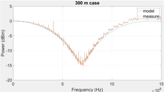
During the test presented in this section it has been put into evidence the bimodal behaviour of the VCSEL 850 nm + SSMF configuration. This bimodality has an impact on the modal interference and modal noise. We can appreciate the behaviour in the measure of the link without any of the previously explained countermeasure in the following figure:

Figure 11: example of bimodal behaviour for a 300 m span.

An analytical model is proposed to characterize such system. It has been demonstrated that a mode filtering at the input section can reduce both modal interference and modal noise. In the case of 300 m SSMF span the bandwidth has improve from 250 MHz to 2500 MHz; instead, the standard deviation of modal noise is reduced to less than 2 dB. The analysis that has been carried out can be exploited for the realization of short-range link with high bit rate but, more important, is a low-cost solution.

1.3) NOTCHES IN FREQUENCY

As we have said in the introduction the bimodal behaviour shows some notches in the frequency in a similar way as the two rays model, even though we are dealing with guided propagation. More specific, the notches in the frequency show an inversional proportional respect to the fiber length. In order to better understand the mathematical behaviour of this effect, let consider a situation where the weight of the two propagating modes is the same so A1=A2. In this case we can formulate as follow:

25

𝑖𝑜𝑢𝑡(𝑡) = ∑ 𝐴2_{𝑖 (1 + 𝑚𝑖 ∗ cos (2𝜋𝑓𝑅𝐹(𝑡 − 𝜏𝑖𝐿1) =}

𝑁𝑚 𝑖

= 2𝐴1 + 2𝐴1 ∗ 𝑚𝑖 ∗ cos (2𝜋𝑓𝑅𝐹(𝜏2 − 𝜏1)𝐿1₂ ) ∗ cos (2𝜋𝑓𝑅𝐹 (2𝑡 − (𝜏1 + 𝜏2)𝐿1₂ ) We have used the prosthapheresis function in order to achieve those results; now in order to find the notches we have to put the first cosine equal to zero.

The cosine at double frequency is ignored for the scope of our dissertation, furthermore we consider the first minima to proceed and the results are the following:

cos (2𝜋𝑓𝑅𝐹(𝜏2 − 𝜏1)𝐿1₂ ) = 0 2𝜋𝑓𝑅𝐹 ∗∆𝜏𝐿₂ =𝜋

2 → ∆𝜏 = 1 𝐿𝑓𝑅𝐹 ∗ 2

So, in general, we can formulate those equation for the minima of the output current [1]:

𝑓𝑚𝑖𝑛, 𝑘 =2𝑘 + 1 2𝐿 ∆𝜏

Hence, we can conclude that this relationship shows that for longer fiber we have more minima, so frequency is inversely proportional to L and in the same way, for increasing frequency we have more minima in parity of L.

1.3.1) INTERMODAL DISPERSION ANALYSYS

The scope of this analysis starts from some detrimental effect that we have observed in the first measure carried out. In order to characterize the effect, we have realized a direct measure (without coupler) of different SSMF span.

We have performed measure at 300m,1500m,3000m,5000m,6500m,8000m and 9500m. All the measures were performed at 4.5 mA bias point of the VCSEL Optowell GS85 single mode. Note that all the following measures has been performed using the same laser.

The different measures were reported in a unique figure to make a comparison among them as follow:

26

Figure 12: panoramic of the different measures from 300m up to 9500 m.

Now we focus on the different set of measurements:

LENGTH GRAPHS

300 m

Delta τ l_span1=300;

deltaTau1=1/(l_span1*2*6.9e8);

27

1500m

Delta τ l_span1=1500;

deltaTau1=9/(l_span1*2*1.25e9)

In this case we pick the 5th maxima for the delta Tau evaluation deltaTau1=2.4000e-12

3000m

Delta τ l_span1=3000;

deltaTau1=19/(l_span1*2*1.3e9); in this case we have picked the 10th minima deltaTau1=2.4359e-12

28

5000m

Delta τ l_span1=5000;

deltaTau1=19/(l_span1*2*7.95e8); even in this case we pick the 10th minima

deltaTau1=2.3899e-12 6500m

Delta τ l_span1=6500;

deltaTau1=19/(l_span1*2*6.11e8) even in this case we pick the 10th _minima

29

8000m

Delta τ l_span1=8000;

deltaTau1=1/(l_span1*2*2.63e7);

the interesting thing is that we use the first minima for delta Tau evaluation like the case of 300m and 1500m. This could be seen not in agreement with the previous cases, in fact we can note a little drift effect between the model and the measure. What is particular in this measure is that, even selecting the frequency where the first minima fall, we were lucky and we pick the correct frequency value. The reason why we were lucky will explained at the end of this tabs.

deltaTau1=2.3764e-12 9500m

Delta τ l_span1=9500;

deltaTau1=37/(l_span1*2*8.1e8)

in this case we pick the 19th minima in order to have a precise evaluation of delta Tau

deltaTau1=2.4042e-12

The reason why we perform this analysis is due to the facts that, increasing the length of the fiber span we notice a strange drift effect in the value of ∆𝜏. Actually, the reason of this

30

misalignment was simply an accuracy factor. In fact, when we perform the measure of ∆𝜏 we select the frequency where the first minima of the measure occur. The measure is actually chosen by an ad hoc selection from the graph that we have just obtained, and this, generates an absolute error in the operation of selecting the frequency. The relative error is the absolute error, that it is always present and is supposed to be the same for each measure, divided by the frequency range from 0 to the selected frequency.

It is easy to understand that, if we pick a minima after the first one, for example the 10th minima, we have the same absolute error but the frequency range is 10 time with respect to the one we would have selecting the first minima.

In the case in the example the relative error will be 10 times smaller respect to the one of the first minima, so the accuracy is way better!

The interesting thing in the 8000m case is that in this case even choosing the first minima we were quite lucky since it was accurate; the reason stands in the fact the frequency of the first minima was picked almost correctly. Even though selecting a frequency from a following minima is always a better solution.

1.4) MATLAB MODELLING FOR

BIMODALITY EVALUATION

In order to study and understand the behaviour of the bimodality that VCSEL 850 nm shows when a SSMF is used as optical channel we have developed a matlab model. This model basically attributes a wight for the 2 mode LP01 and LP11 that propagates inside the optical channel. A preliminary assumption, that will be demonstrated in the next section, is that the mode carrying the most power is always the principal mode LP01.

The analysis regards the use of the coupler instead of the SMF 5um fiber span in order to compensate the bimodality. This solution represents an attractive idea because can mitigate the problem of bimodal behaviour and also opens new applicative scenarios like feedback predistortion of the laser that will be investigated in the next chapters.

31

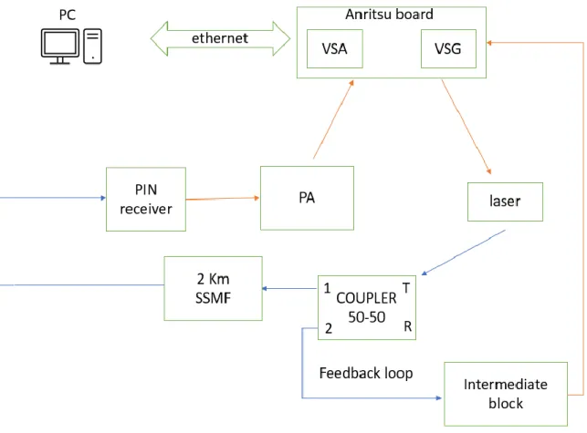
Figure 13: schematic of the experimental set up of the final system. The blue link represents optical connections,

while the orange link represents the electrical ones. The red arrow represents electrical connections, the blue ones represent the optical connections.

All the coupler in our analysis are 1550 nm couplers and present two inputs, called T and R, and two output called 1 and 2. Note that the intermediate block, is actually a full receiving chain, including the PIN receiver, the power amplifier and the electronics that perform a demodulation and detection of the signal and do some elaboration on the baseband signal in order to apply the predistortion algorithm to the system. In addition to the previous features, the intermediate block has also to re-create the transmitting signal and modulate the transmitting laser. In our practical case we do not have any intermate block, in fact the Anritsu board adopted for our work, has only one receiving port. For the realization of the final set up in practice we have trained the algorithm using the feedback loop and using the receiving port of the Anritsu board for the receiving chain e for the transmission of the signal with the laser. Once the training is finished, we switch the connection from the feedback port of the coupler to the direct one (T1), then we have simply pre-distort the signal applying the coefficients evaluated in the feedback loop for the direct via.

32

All the measurements were carried out in the same way for each coupler (50-50, 90-10 and 99-01) and for each span of fiber, in our case 300 m and 2km.

The first measurement is always the one without coupler that represents the starting situation where the bimodal behaviour shows its notches. Once the starting measure is done, we measure the behaviour for the other four configurations of the coupler T1, T2, R1 and R2, in order to realize a complete analysis.

All the analysis has been carried out using a fixed scheme: • Measurements

• Import the measurements to matlab

• Graphical representation of the four configurations of the coupler • Weight modes analysis

The link can be schematized in figure as follow:

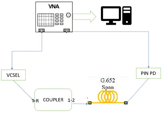
Figure 14: Schematic of the experimental set up implemented in the first measures.

We can see the VNA that is the origin and final point of the connection, then we have a VCSEL operating at 850 nm connected to a coupler 50-50 designed for operating at 1550 nm and

33

connected to a SSMF fiber. At receiving side, we denote a PIN rx operating at 12 V that is connected to the receiving port of the Anritsu.

The standard procedure is given as follow; we first load the file into matlab:

%% import data close all clear all datab2b=importdata('VCSEL_sm_4.5ma_rxoptwell_b2b.s2p', ' ',5); data300m=importdata('VCSEL_sm_4.5ma_rxoptwell_300m.s2p',' ',5);

Then we extract the data from the matrix that is imported in the Matlab workspace and we extract the back-to-back(b2b) data and the data corresponding to the length we want to analyse. As we can see in the Matlab code we subtract to the measure at the given length the b2b measure in order to characterize the optical link, subtracting the behaviour of transmitter and receiver.

%% extraction of data from back2back

freqb2b=datab2b.data(:,1); s21realb2b=datab2b.data(:,4); s21imagb2b=datab2b.data(:,5); s21magnitudeb2b=abs(s21realb2b+i*s21imagb2b); s21magb2bdB=mag2db(s21magnitudeb2b);

%% extraction of data from new measure without coupler

freqBase=data300m.data(:,1); s21realBase=data300m.data(:,4); s21imagBase=data300m.data(:,5); s21magnitudeBase=abs(s21realBase+i*s21imagBase); s21magBasedB=mag2db(s21magnitudeBase); diffBase=s21magBasedB-s21magb2bdB;

Then we proceed with the graphical representation of the data just put inside the simulator. The core of the matlab program is the weight evaluation of the 2 mode that is carried out in an iterative way as we can appreciate in the matlab script that follows:

%% calculation of coefficient without coupler 300m

l_span1=300;

deltaTau1=1/(l_span1*2*6.9e8);

34 figure plot(freq300m,y.^2) z=mag2db(abs(y)); figure plot(freq300m, z); tau1=5e-9; tau2=deltaTau1+tau1; %t=[0 : 1e-9 : 0.2]; t=linspace(0,0.00001, 1601); a_1=1; a_2=1; modindex=1; %for a_2 =[0:0.1:1] for i = (1:length(freq300m))

m(:,i)=(a_1)^2*(modindex * cos( 2*pi*freq300m(i)* ( t - tau1*l_span1)))+(a_2)^2* (modindex * cos( 2*pi*freq300m(i)* ( t - tau2*l_span1))); end figure plot(t, m(:,i)); for a_2=[0.6:0.01:0.63] a_1=sqrt(1-(a_2)^2);

Ac=modindex* (( a_1)^2 * cos(2*pi*freq300m* tau1* l_span1)+ (a_2)^2 * cos (2*pi*freq300m*tau2*l_span1));

As=modindex* (( a_1)^2 * sin(2*pi*freq300m* tau1* l_span1)+ (a_2)^2 * sin (2*pi*freq300m*tau2*l_span1));

envelopemod=sqrt(Ac.^2+As.^2); envelopnorm=envelopemod/envelopemod(1); envelopnormdB=mag2db(envelopnorm); figure plot(freq300m,envelopnormdB); hold on delta1db=diffBase300m - diffBase300m(10); plot(freq300m,delta1db); end

For shake of simplicity we consider the modulation index mi equal to 1. This simplification makes sense because we normalize the measurement. Note that the mi just consider is different from the m variable present in the code.

35

The mathematical model is developed as we have analyse in the section 1.1.1; the value m(:,i) represents the total output current, instead the Ac and As value represents the real and imaginary part of the envelope of I,outRF.

The value a_1 and a_2 represents the weights of the and their square value represent the actual power splitting ratio of the 2 mode LP01 and LP11 and will be indicated as A1 and A2.

Those coefficients are in a strict relation with each other, in fact we assume a normalization condition such that _𝐴12_{+ 𝐴2}2 = 1 as we can see inside the second for loop where the iterative procedure is realized.

Basically, it is a fitting problem in which we play with the coefficients A1 and A2 such that, the modelled curve, fit in the best possible way with respect to the measured value; this way we can characterize the weights of the two propagating modes and understand if the coupler acts somehow as a mode filtering or not.

Then a complete analysis using the 3 couplers previously mentioned is carried out for 300 m and 2 km case.

1.5) 300 m CASE ANALYSIS

The second analysis has been carried out for the 300 m case SSMF span. Differently from the previous set of measures, from this point, in all the measure a coupler will be present. In particular, we have performed a complete analysis of the three couplers in its four configurations. The final goal of this part is to extract a value of the weights of the 2 modes entering inside the SSMF fiber. All the three couplers analysed operate at 1550 nm so will not act as we could expect for the 850 nm case. The first study case is the coupler 50-50. The analysis performed will be the same for each case.

36

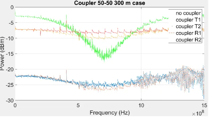
1.5.1) COUPLER 50-50

In figure 15 and 16 we observe the behaviour of the normalized link and the non-normalized one respectively:

Figure 15: normalized measure.

37

Now we proceed the analysis with the 4 configurations of the coupler:

case Graph Power

weights No coupler A1=0.6156 A2=0.3844 T1 A1=0.9682 A2=0.0318 T2 A1=0.8775 A2=0.1225

38 R1 A1=0.7975 A2=0.2025 R2 A1=0.8400 A2=0.16 1.5.2) COUPLER 90-10

As before we start the analysis with the graph of the normalized and non-normalized curve; then the different configuration will be taken into account.

39

Figure 18: Non-normalized measure.

Analysis of the different configurations:

case graph Power

weights No coupler A1=0.6156 A2=0.3844 T1 A1=0.7975 A2=0.2025

40 T2 A1=0.84 A2=0.16 R1 A1=0.96 A2=0.04 R2 A1=0.84 A2=0.16

41

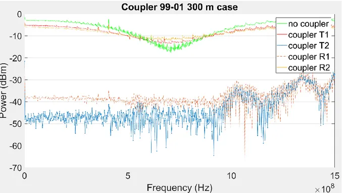
1.5.3) COUPLER 99-01

As before we start the analysis with the graph of the normalized and non-normalized curve; then the different configuration will be taken into account.

Figure 19: normalized curve.

42

Analysis of the different configurations:

case graph Power

weights No coupler A1=0.6156 A2=0.3844 T1 A1=0.6975 A2=0.3025 T2 A1=0.96 A2=0.04

43 R1 A1=0.96 A2=0.04 R2 A1=0.75 A2=0.25 1.5.3) CONCLUSION ON 300 m

Actually, the measures carried out were a lot more but here are presented the last set of measure that represents the more accurate case analysis. In fact, from the first sets of measure we have notice that in order to guarantee an accurate result, we have to fix all the fiber span, in order not to move since each movement can stimulate in a different way the two mode presents inside. For the shake a completeness we have collected al the results in an excel file, with a column for the coefficients used in the algorithm and a column for the power coefficients that are the square of the previous ones.

44

Tab 2: it shows a comparison between two set of measures with coupler 50-50, the first and third

column.represent the splitting coefficients, the second and forth represent their square value also called power splitting.

Tab 3: it shows a comparison between two set of measures with coupler 90-10, the first and third column

represents the splitting coefficients, the second and forth represent their square value also called power splitting.

Tab 4: it shows a comparison between two set of measures with coupler 99-01, the first, third, fifth and seventh

column represents the splitting coefficients, the second, forth, sixth and eighth represent their square value also called power splitting.

45

For the last coupler (99-01) we have performed also a further analysis for the worst and lucky case.

For worst we intend a case where the 2 mode LP01 and LP11 carries actually the same amount of power, for lucky we mean a case where the mode LP01 is dominant as we can see in the table:

worst lucky

1.6) 2 KM ANALYSIS

Now the same analysis just seen is repeated with the 2 km SSMF fiber strand. The results are collected as before:

1. Coupler 50-50 2. Coupler 90-10 3. Coupler 99-01

46

1.6.1) COUPLER 50-50

The first results collected are as before the normalized and non-normalized measured of the different configurations:

Figure 21: normalized measure 2 km case.

47

Then the 4 different configurations are analysed:

case graph Power

coefficients No coupler A1=0.5511 A2=0.4489 T1 A1=0.8976 A2=0.1024 T2 A1=0.7296 A2=0.2704

48 R1 A1=0.6751 A2=0.3249 R2 A1=0.8775 A2=0.1225 1.6.2) COUPLER 90-10

In the same way as before we first present the normalized and denormalized measurements:

49

Figure 24: Non-normalized measure 2 km case.

Now we proceed with the 4 different configurations of the coupler:

case graph Power

weights No

coupler

A1=0.5511 A2=0.4489

50 T1 A1=0.7884 A2=0.2116 T2 A1=0.9375 A2=0.0625 R1 A1=0.9375 A2=0.0625

51

R2 A1=0.7975

A2=0.2025

1.6.3) COUPLER 99-01

Normalized and non-normalized measurements:

52

Figure 26: Non-normalized measure 2 km case.

Analysis of the different configurations:

case graph Power

weights No coupler A1=0.5511 A2=0.4489 T1 A1=0.8844 A2=0.1156

53 T2 A1=0.96 A2=0.04 R1 A1=0.96 A2=0.04 R2 A1=0.8556 A2=0.1444

54

1.6.4) MEASURE COMPARISON

In order to compare the different couplers we have collected all the data inside a tab in order to see the different.

Tab 5: the tab shows a comparison for the power splitting coefficients with the three different couplers tested.

1.7) CONCLUSION ON THE TWO

MEASURMENTS SET

After the two complete analysis of 300 m and 2 km SSMF we can conclude that the coupler act somehow like a mode filtering. In all the test realized so far, we have supposed that the principal mode LP01 is the dominant one so the coefficient of A1 will always bigger than A2. This assumption will be demonstrated in the following sections.

After the experiment carried out, we can conclude that, all the couplers somehow filter the LP11 mode, anyway our final scope is to realize a predistortion using the feedback branch so even the output power level becomes important.

Both in 300 m and 2 km we can appreciate that the feedback path, corresponding to T2 or R1 configuration, has different power level in function of which coupler we are considering. In order to realize a feedback predistortion, we need sufficient power on the T2 or R1 configuration, so in this case the most suitable solution will be to implement the coupler 50-50 in our system in order to have enough power on the feedback path.

55

1.8) 5 um TEST

In order to demonstrate that the most dominant mode is LP01 as we have supposed, and also to make a comparison with the initial solution already proposed in the literature, where a small strand of 5 um SMF is placed at the input section of SSMF. So the system can be represented as follow:

Figure 26: schematic of the tested link with SMF 5 um.

we have already analysed the effect of 5 um from a theoretical point of view, now we modify the previous scheme in order to realize a further analysis.

In the following tabs it is presented a comparison between the three different couplers with this particular configuration:

56

COUPLER Graph normalized

50-50

90-10

57

COUPLER Graph non-normalized 50-50

58

99-01

We do not show the results of the analysis of the four configurations of each coupler since the starting 5 um SMF basically filter out all the LP11 mode so all the four configuration presents a flat behaviour, demonstrating the presence of LP01 only.

1.8.1) CONSIDERATION ON 5 um SMF

A further experiment has been carried out in order to understand a strange behaviour we have encountered during the measurements. Basically, a measurement of the power was carried out at the laser output section and on the two output paths going out from the coupler, for example T1 and T2. We should expect that the collected power on the two paths is the same as the output laser but actually what we measure was 3 dB lower with respect to what we expected.

In order to better understand this behaviour, we have repeated the test inserting the 5 um SMF between the laser and the SSMF fiber and repeat the measurements of power.

A first measure is taken at the input section of the coupler so just after the 5 um SMF fiber and a second set of measure has been carried out at the two output of the coupler, T1 and T2.

59

Figure 28: schematic of the second measure.

We have transmitted 8 dBm from the laser and the measure at the input of the coupler was -8.34 dBm.

Then the second measure was carried out with the following results: P at T1: -8.93 dBm → 127.8 uW

P at T2: -17.3 dBm → 18.48 uW

If now we sum together the linear power and we reconverts it in dBm we found -8.349 dBm. In this case we do not have the 3 dB losses observed in the first case.

In conclusion we can assert that the loss is given by the LP11 mode only, that somehow convert into radiant mode, causing the 3 dB loss we have observed in the first case.

This experiment also demonstrate that the most dominant mode is the LP01 so the assumption we have taken in all the previous measure of assuming A1 always greater than A2 it is valid. The limit case of power weights is represented by the case with no coupler where we have half power coming from LP01 and half power coming from LP11.

1.9) CONCLUSION

In this chapter we first put into evidence the possible application of this new solution for low-cost Radio-Over-Fiber system. Initially, a study of the state of art of this technology has been performed to show the technical solution implemented nowadays. The analysis performed on the differ couplers shows that can behave somehow like a mode-filter. Our final goal is to realize a predistortion system that exploits the feedback path, so even the power going out from this via assume an important role. For our scope, the best solution is the coupler 50-50 that present 10-15 dB more, respect to the 90-10 or 99-01, from the feedback path.

In the next chapter we will focus on the actual predistortion algorithm realized from this architecture and how the performance can be improved using this technical solution.

60

CHAPTER 2 DIGITAL PREDISTORTION

2.1) OVERVIEW ON PREDISTORTION

The scope of this dissertation is to explain theoretically and experimentally the benefit coming from digital predistortion of the link itself. The idea is to enhance the linearity of short and medium link for the Mobile Front Haul links already present in the mobile communication system. As seen before it will be used a VCSEL operating at 850 nm and the standard single mode fiber SSMF, in order to maintain a low-cost and low-consumption solution for the RoF link.

In this dissertation the memory polynomial (MP) is used together with Indirect Learning Architecture (ILA). The performance improvement is measure through some significative quantities like Adjacent Channel Power Ratio (ACPR), Normalized Mean Square Error (NMSE) and Error Vector Magnitude (EVM).

The Radio over Fiber technology can be exploited for long range and short-range communication, anyway the focus of this work is for short range link. In this kind of link, the main part of the non-linearities comes from the laser source and the photodiode, placed at the receiver. All the other non-linearities can be neglected for the shake of simplicity, since they do not affect the link in a significative way [6].

The effect of the non-linearity leads to a distortion in-band and out of band, this damage the link quality and raise the interference among the channels.

There are different techniques for predistortion that will be explained in the next sections, anyway among the different techniques we focus on Digital Predistortion (DPD). The basic idea behind the DPD is to adopt a digital pre-distorter able to recreate an opposite non-linear characteristic of the RoF link.

This way the cascade pre-distorter + RoF link has a linear behaviour. Note that the next graph is referred to a PA, not the full RoF link, anyway the idea of digital predistortion remain the same and can be appreciated in the following figures:

61

Figure 29: AM/AM and AM/PM characteristics of PA and DPD [16].

In the context of this dissertation the DPD is applied for an LTE application in order to increase the linear behaviour. In general, DPD is applied to the PA that become strongly non-linear with wideband, high envelope signals like those of LTE. In this particular case, the DPD algorithm, is applied to the whole RoF link, including transmitting laser, PA and PIN receiver.

The VCSEL laser chosen for this work as already seen is low cost and low consumption but has a serious problem because of its small dynamic. In fact, LTE signal presents signal with a high value of Peak-to-Average Power Ratio (PAPR) and this create a problem with the small

62

dynamic of the laser since the peak of the signal can be so high with respect to the mean value, that can be subjected to strong non-linearity.

In order to characterize the nonlinear model, we use memory polynomial since a memoryless model would not be enough accurate to describe the electro-optic conversion. The MP model will be further investigated in the next section and represents a special case of Volterra series. The DPD model identification used is Indirect Learning Architecture and it is structured like the scheme presented in figure 30.

Figure 30: ILA architecture model.[6]

The MP is applied as follow:

𝑥(𝑛) = ∑ ∑ 𝑎𝑘𝑞 ∗ 𝑢(𝑛 − 𝑞) ∗ |𝑢(𝑛 − 𝑞)|𝑘−1 𝑄 𝑞=0 𝐾 𝑘=1 𝑧𝑝(𝑛) = ∑ ∑ 𝛾𝑙𝑚 ∗ 𝑧(𝑛 − 𝑚) ∗ |𝑧(𝑛 − 𝑚)|𝑙 𝑀 𝑚=0 𝐿−1 𝑙=0

DPD model is based on the estimation of the coefficients presents in those two formulas; anyway, in ILA post-inverse can be used as pre-inverse and this permits to realize a linear estimation of the coefficients. Obviously, the training phase, where the coefficients are estimated, can be done offline it the system does not change in time.

In this architecture the first evaluation is for the post distorter coefficients, then the pre-distorter is updated. In order to complete the overview, we focus on the figure of merit that are exploited to evaluate the performance improvement:

63

• 𝑁𝑀𝑆𝐸𝑑𝐵 = 10𝑙𝑜𝑔10(∑𝑁𝑛=1|𝑥(𝑛)−𝑧𝑝(𝑛)|2

∑𝑁 |𝑥(𝑛)|2

𝑛=1 ) the NMSE is evaluated between the

estimated post distorter output zp(n) and the pre-distorter output x(n). N represents the length of the signal.

• 𝐴𝐶𝑃𝑅𝑑𝐵 = 10𝑙𝑜𝑔10(∫ 𝑆(𝑓)𝑑𝑓

𝑎𝑑𝑗𝑎𝑐𝑒𝑛𝑡𝐵𝑎𝑛𝑑𝑢𝑝 𝑎𝑑𝑗𝑎𝑐𝑒𝑛𝑡𝐵𝑎𝑛𝑑𝑙𝑜𝑤

∫𝑢𝑠𝑒𝑓𝑢𝑙𝐵𝑎𝑛𝑑𝑢𝑝𝑆(𝑓)𝑑𝑓

𝑢𝑠𝑒𝑓𝑢𝑙𝐵𝑎𝑛𝑑_𝑙𝑜𝑤

) in this case S(f) represents the power

spectral density of the output signal y(n). • 𝐸𝑉𝑀𝑑𝐵 = √∑𝑁𝑘=0(𝐼𝑘−𝐼̅𝑘)2+(𝑄𝑘−𝑄̅𝑘)2

∑𝑁 _𝐼𝑘2_+𝑄𝑘2 𝑘=0

this equation operated directly on the constellation, in fact I and Q represents the transmitted component, instead 𝐼̅ and 𝑄̅ represent the received components respectively of the in-phase and quadrature via. N represents the number of samples and k is the index of the sum operator.

2.1.1) LINEARIZATION METHODs

There are different linearization techniques available for our purpose, they can be classified as the following scheme:

64

They have different characteristic but the same final purpose, let’s look more in detail the different techniques [7]:

• Electrical linearization: it can be split in analog pre-distortion and digital linearization that will be discussed next. For the analog case, the idea is to create a predistortion circuit that suppress the intermodulation product that are particularly dangerous, since fall close to the useful bandwidth. In general, the intermodulation product of third order (IMD3), are in antiphase with respect to the RF signal so, the analog predistortion circuit, generates IMD3 components in phase with the signal [7] in order to cancel out the original IMD3. Usually to achieve a broadband linearization, Schotty diodes are implemented since their ability to generate all order nonlinearities.

• Optical linearization: it can be differentiated into mixed-polarization, dual wavelength and optical channelization [7]. This technique is able to cancel out both second and third order nonlinearities. The linearization bandwidth is only limited by the bandwidth of the optical modulator, anyway we do not enter inside this technological solution since it is out of the scope of this dissertation.

• Digital linearization: the goal is always to suppress the IMD3 generated by RF power amplifiers. This technique exploits the analog-to-digital converter (ADC) to sample the analog signal and realizing digital signal processing on the samples. For this reason, the actual band that can be linearized, is limited to 100 MHz [7], due to the limits in the sampling frequency of the ADC. Actually, it is possible to achieve greater bandwidth but the DSP, using for instance the Lagrange procedure, require complex calculation and a big power consumption. The principle of digital predistortion techniques is that the pre-distorter generates an inverse nonlinear characteristic in order to compensate the RoF transmission. Anyway, when broadband signals are transmitter over RoF system the memory effects start to be not negligible.

In general, Volterra series is adopted to estimate the behaviour of the RoF link and in general all non-linear dynamic system. In practical case some other techniques will be implemented because of the huge calculation complexity of Volterra analysis.

The most adopted solution is the memory polynomial, as the one we use for our dissertation, that allows to reduce a lot the computational complexity, reaching a good accuracy level.