Modeling and model validation of supercapacitors for real-time simulations

ALMA MATER STUDIORUM - UNIVERSITÀ DI BOLOGNA

SCHOOL OF ENGINEERING AND ARCHITECTURE

Department of

Electrical, Electronic and Information Engineering “Guglielmo Marconi”

DEI

Electrical Engineering

MASTER THESIS in

Photovoltaic Conversion and Storage of the Electrical Energy

MODELING AND MODEL VALIDATION OF

SUPERCAPACITORS FOR REAL-TIME SIMULATIONS

Presented by: Supervisor:

Simone Pezzolato Prof. Dr.-Ing. Antonio Morandi

Co-Supervisors:

Shahab Karrari Dr. Giovanni De Carne

Prof. Dr.-Ing. Mathias Noe Prof. Dr.-Ing. Pierluigi Ribani

Academic Year 2018/2019 Session III

2

Table of Content

1 Chapter 1: Introduction to Supercapacitors ... 7

1.1 Structure and Operation Principle ... 7

1.1.1 Molecular point of view ... 7

1.1.2 Energy storage ... 9

1.2 Applications of Supercapacitor Energy Storage Systems ... 10

1.3 Common operation modes of supercapacitors ... 13

1.3.1 Constant current ... 13

1.3.2 Constant power ... 18

2 Chapter 2: Modeling of Supercapacitor Cells ... 24

2.1 Equivalent-circuit Modeling of Supercapacitors ... 24

2.1.1 The RC series model... 25

2.1.2 The Two-Branch model ... 26

2.1.3 The Zubieta model ... 27

2.1.4 The Series model ... 29

2.2 Model Validation ... 32

2.2.1 Description of Supercapacitor ... 32

2.2.2 Experimental Setup ... 36

2.2.3 Parameter Estimation Procedure ... 39

2.2.4 Comparison between Models ... 40

3 Chapter 3: Real-Time simulation of Supercapacitor ... 61

3.1 Real-Time simulation and its applications ... 61

3.2 Real Time implementation and setup ... 69

3.3 Real-Time Simulation of a Single cell ... 74

3.4 Real-Time Simulation of Supercapacitors Stacks ... 76

3

Table of figures

Figure 1.1 Schematic of a supercapacitor cell ... 7

Figure 1.2 Helmholtz Double Layer model (left), Model of the Supercapacitor (right) ... 9

Figure 1.3 Examples of topologies using supercapacitors to have a more performant ESS: a) Series topology; b) Parallel passive topology; c) Parallel active topology (direct connection of ESS to the DC bus); d) Parallel active topology (both ESS with a PCS) . ... 11

Figure 1.4 RC series equivalent circuit of a supercapacitor cell ... 13

Figure 1.5 ESR is responsible for the voltage step that occurs across the SC ... 14

Figure 1.6 Voltage response of the supercapacitor with the shown input current pulses ... 14

Figure 1.7 Equivalent circuit for the discharging phase ... 15

Figure 1.8 Supercapacitor efficiency in a constant current operation ... 17

Figure 1.9 Voltage behaviour with constant power neglecting the ESR ... 19

Figure 1.10 Constant power injection and extraction ... 19

Figure 1.11 Current behaviour with constant power ... 20

Figure 1.12 Power and Current in the first cycle ... 21

Figure 1.13 Voltage response taking into account the ESR ... 22

Figure 1.14 ESR voltage drop difference: on the left the drop at minimum voltage is represented instead on the right that one at the maximum voltage ... 22

Figure 1.15 Efficiency as function of the current ... 23

Figure 2.1 RC model ... 25

Figure 2.2 The Two-Branch model... 26

Figure 2.3 Simplified Two-Branch model ... 27

Figure 2.4 The Zubieta model... 28

Figure 2.5 The Series model ... 29

Figure 2.6 Example of Lookup-table ... 30

Figure 2.7 ESR and Capacitance as function of the temperature. Courtesy of picture: Maxwell Technologies 34 Figure 2.8 Cell structure from data-sheet. Courtesy of picture: Maxwell Technologies ... 35

Figure 2.9 Cell structure from data-sheet(2). Courtesy of picture: Maxwell Technologies ... 35

Figure 2.10 Experiment setup ... 36

Figure 2.11 Shift got after the first cycle. ... 37

Figure 2.12 Input current pulses sequence. ... 38

Figure 2.13 Voltage measured across the component during the experiment ... 38

Figure 2.14 Simulink model of the Zubieta model ... 39

Figure 2.15 The RC model ... 40

Figure 2.16 RC series model voltage comparison... 41

Figure 2.17 RC series model absolute error ... 42

Figure 2.18 RC series model percentage relative error ... 43

Figure 2.19 Percentage relative error density distribution ... 43

Figure 2.20 Two-Branch model ... 44

Figure 2.21 Two-Branch voltage comparison ... 45

Figure 2.22 Second positive peak ... 46

Figure 2.23 Peak of the second peak ... 46

4

Figure 2.25 Two-Branch absolute error and percentage relative error ... 47

Figure 2.26 Two-Branch density distribution ... 48

Figure 2.27 Zubieta model ... 49

Figure 2.28 Density distribution of the percentage relative error of the Zubieta model ... 50

Figure 2.29 Percentage relative error of the Zubieta model ... 50

Figure 2.30 Series model ... 51

Figure 2.31 Voltage comparison with Series model output and experimental voltage ... 53

Figure 2.33 Density distribution of percentage relative error of the Series model ... 54

Figure 2.32 Percentage relative error of the series model ... 54

Figure 2.34 Voltages comparison of all the models ... 55

Figure 2.35 Detail of voltages in the first two peaks ... 56

Figure 2.36 Detail of voltage in the third peak ... 56

Figure 2.37 Relative error comparison of all the models... 58

Figure 2.38 Density distributions comparison ... 59

Figure 3.1 Controller Hardware-in-the-Loop (CHIL) and Power Hardware-in-the-Loop (PHIL). ... 62

Figure 3.2 Capability requirements (a) and time-step requirements for different systems ... 63

Figure 3.3 Example of hardware type A ... 64

Figure 3.4 Hardware architecture of eMEGASIM real-time simulator ... 65

Figure 3.5 Inverter power analysis inside a photovoltaic system with power hardware in the loop ... 68

Figure 3.6 Example of blocks division for RT-Lab. Picture courtesy of: Opal-RT Technologies ... 69

Figure 3.7 Example of Computation and GUI blocks. Picture courtesy of: Opal-RT Technologies... 69

Figure 3.8 Grouping into subsystems. Picture courtesy of: Opal-RT Technologies ... 70

Figure 3.9 Monitor window. Picture courtesy of: Opal-RT Technologies ... 70

Figure 3.10 Correct time step. Picture courtesy of: Opal-RT Technologies ... 71

Figure 3.11 Overrun occurring. Picture courtesy of: Opal-RT Technologies ... 71

Figure 3.12 Two-Branch model implementation for the RT-Lab platform ... 72

Figure 3.13 Example of the computation block of the Two-Branch model with three parallel branches with two series supercapacitor models each one ... 72

Figure 3.14 OP4510. Picture courtesy of: Opal-RT Technologies ... 73

Figure 3.15 RC series model maximum execution times ... 77

Figure 3.16 Two-Branch model maximum execution times ... 78

Figure 3.17 Zubieta model maximum execution times ... 80

Figure 3.18 Series model maximum execution times ... 82

Table of Tables

Table 2.2 Dimensions of the supercapacitor cell ... 35

Table 2.3 The estimated parameters for the RC model ... 40

Table 2.4 Parameters of the distribution function of the RC series model ... 44

Table 2.5 Two-Branch model estimated parameters ... 45

Table 2.6 Parameters of the Two-Branch relative error density distyribution ... 48

Table 2.7 Estimated parameters of the Zubieta model ... 49

Table 2.8 Parameters of the percentage relative error density distribution of the Zubieta model... 51

5

Table 2.10 Coefficients values for the construction of the lookup tables ... 52

Table 2.11 Parameters of the density distribution of the percentage relative error of the Series model ... 55

Table 2.12 Parameters of the density distributions of all the models ... 60

Table 3.1 Real-time model execution time for single cells of supercapacitor models ... 74

Table 3.2 The model execution times for supercapacitors stacks using the RC series model ... 76

Table 3.3 The model execution times for supercapacitors stacks using the Two-Branch model. ... 78

Table 3.4 Zubieta model real-time simulation values ... 80

Table 3.5 The Series model execution times for supercapacitors stacks using the series model ... 81

Table of Equations

6 Abstract

Supercapacitors are becoming very important in the automotive and energy and power industry due to their specially characteristics, in particular in the field of hybrid vehicles and hybrid energy storage systems. For this reason, having accurate models that can represent the behavior of such systems is necessary and the main important characteristics of supercapacitor are a high-power density and a long lifetime with low maintenance. This thesis focuses on modeling supercapacitors to the study of their behavior in a short time period. As, their operation often short intense power

deliveries. The goal of this thesis is to compare the accuracy of equivalent-circuit models of supercapacitors together with their required execution time for real-time simulations.

In the first chapter, the operation of the supercapacitor from the molecular point of view and the principal of storing energy in a supercapacitor is introduced. Common operation modes of supercapacitors are also introduced. Next, equivalent-circuit models of supercapacitors are

introduced. The models are implemented in MATLAB/Simulink and their responses are compared with the experimental results. The parameter estimation results. The parameter estimation tool of MATLAB has been used to estimate the model parameters for each model. At the end, the models are compared in terms of inaccurately reproducing the experimental response of a supercapacitor. Lastly, the models are compared in terms of their required execution time for real-time simulations. The models are implemented in RT-LAB software and simulated on the Opal-RT’s OP4510 real-time simulator. Here the execution real-times of the models compared with the goal of representing a large number of supercapacitor cells.

7

1 Chapter 1: Introduction to Supercapacitors

1.1 Structure and Operation Principle

The supercapacitor is a system composed by two metallic collectors in the extreme parts. These collect and distribute the current. Going toward the center there are porous carbon made electrodes (μm), then the electrolyte. In the mid of the electrolyte there is a separator, permeable for ions, in order to not have a short circuit among electrodes. The schematic of a supercapacitor cell is shown in

Figure 1.1 [1].

The structure is similar to that one of a battery, but it has not reacting materials.

In the batteries there is a plate charging negatively because there is a natural oxidation reaction: some atoms lose their electrons leaving them in the electrode. They are now available for the conduction and take part to the adjacent solution. In the cathode occurs the opposite reaction: some atoms

1.1.1 Molecular point of view

8

acquire the electrons. This charge configuration will create its own potential configuration. There is a potential gradient; in the middle the potential remains constant being the electrolyte an inert

conductor and finally there is another gradient. The voltage on the system is the no-load voltage across the electrochemical battery (∆V).

In the building of a supercapacitor, cause the use of inert materials, positive and negative ions remain randomly located. There is not charge thickening and so there is not a voltage across terminals. However, applying a voltage across the component a current is generated and some electrons leave an electrode going toward the other. This is a physical charge shifting. A plate is charging positively, and negative ions thickening around occurs. Electrons carried by the electromotive force in the other plate charge it negatively. Close to this electrode positive ions are attracted. A double charge layer is created, like a capacitor. It is like to have the positive charges distribution (being part of the electrode structure), the negative charges distribution in the electrolyte made by anions and cations with

absorbed molecules. A negative ion has around solvent polar molecules. This molecule has both positive and negative parts, but it is globally neutral but with different barycenter for positive and negative charge. This is an electric dipole interacting with the cation surrounding it.

This set of surrounded particles go close to the electrode staying yet at a distance of a molecular layer called “Double Layer” (≈10−10_{𝑚). In the detail, this can tell us that being the distance very}

low, the capacitance will be high. The surface is also affecting the capacitance. In fact, the surface is very huge due to porous carbon. Its surface is full of irregularities. These make the final value much greater.

9

This structure is called “Helmholtz Double Layer”. This is represented by a series of a capacitor, a resistance and finally another capacitor. There are also two parallel resistances in parallel with the two capacitors, representing the self-discharge behavior on those interfaces.

The equivalent circuit is summed up to a capacitance with a parallel resistance, and an equivalent series resistance playing a basic role in the efficiency of the component. This simplification is since the two RC parallels are almost similar, so the current splitting can be represented in a unique parallel. Every capacitance is given by:

𝐶 =ɛ ∙ 𝑠 𝑑

1.1

1.1.2 Energy storage

10

Where is it ‘ɛ’ is the permittivity of the dielectric, ‘s’ is the surface and ‘d’ is the distance. So, the capacitance will be high having a very low distance (≈ μm) and a very high surface given by the porous carbon, into which the liquid conductor leaches. There are lot of holes in the powder that is enough compact to create an electric continuity and at the same time to increase the surface by means of the great deal of holes (𝑆 ≈ 3000 𝑚2_{/𝑐𝑒𝑙𝑙 ).}

For example, a Maxwell BCAP (Cn=3000F, Vn=2.7V, ESR=0.29mΩ) has 𝑊_𝑛 = 1

2𝐶𝑉

2 _{= 10,9𝑘𝐽 ≈ 3𝑊ℎ}

This value is the rated energy stored in the capacitor.

A capacitor can be used till his voltage is remaining higher than a threshold value, which usually is the half of the rated voltage

𝑉_𝑚𝑖𝑛 =1 2𝑉𝑛

1.2 So, the available energy is

∆𝑊 =1 2𝐶𝑉𝑛 2_- 1 2𝐶𝑉𝑚𝑖𝑛 2 _{= 75% 𝑊} 𝑛 1.3

1.2 Applications of Supercapacitor Energy Storage Systems

Large applications for supercapacitors can be found in microgrids. Renewable sources are in great expansion due to the environmental impact which is one of the issues to which many countries pay close attention. The production targets with renewable sources are of great importance and the management of these systems goes hand in hand with their expansion. The problem with renewable sources is that they do not guarantee constant energy production over time. This in turn is a source of

11

great problems for electricity grids because it is the cause of continuous electricity quality disturbances. Moreover, it affects the stability and reliability of the systems. Microgrids, in

particular, are small systems that can be connected directly to the network or operate in an islanded manner. They often integrate large amounts of ESS. These networks need both great energy and great power density: this is why often just one ESS is not enough, so we get to use more than one of these systems together. This gives rise to HESSs (Hybrid Energy Storage Systems).

Figure 1.3 shows four configurations of ESS. Figure 1.3a)[2] and Figure 1.3b)[3] represent simpler

topologies, while Figure 1.3c) and Figure 1.3d) represent more complex systems [4]. In particular,

hybrid storage systems constituted of Vanadium Redox Batteries (VRB) and supercapacitors, connected to energy production systems with Permanent Magnets Synchronous Machine (PMSM).

The contribution of supercapacitors is very important as they are sources of high-power density in a short time, while other systems deal with the amount of energy in longer times. Energy management is very important in these microgrids. There are converters, which require particular attention in the

Figure 1.3 Examples of topologies using supercapacitors to have a more performant ESS: a) Series topology; b) Parallel passive topology; c) Parallel active topology (direct connection of ESS to the DC bus); d) Parallel active topology (both ESS with a PCS) .

12

construction choices, and an energy optimization system is always needed in order to better coordinate the microgrid. This gives the possibility to better meet the requirements of stability and good functioning of the network [5].

SCs are also used in UPSs because they offer performance that batteries cannot achieve. Often the two are used together. Indeed, SCs can provide energy during short outages better than batteries. In addition, this will extend the life of the batteries. Sometimes UPSs also have only supercapacitors, because with sensitive loads they are sufficient and have lower maintenance costs.

The SCs can be used as energy recovery means for elevators and cranes. In fact, in these cases the energy can be recovered in the downward phases. The supercapacitors are therefore adequate because they allow energy recovery in a short time and are able to supply large currents which is what is needed in these applications.

The automotive industry is also an area in which SC are increasingly taking hold. Here too, as in the previous cases, it is possible to combine the use with batteries. Their use varies from low energy consumption applications to applications with a higher energy level. Their combination with batteries offers numerous advantages, including greater power, greater energy recovery and longer battery life thanks to the leveling of charge cycles. This is a leading sector for the use of

13

1.3 Common operation modes of supercapacitors

The voltage response of the supercapacitor is analyzed using the equivalent circuit with a capacitance and series resistance shown in Figure 1.4. The parallel resistance is neglected, because it is taking into

account the self-discharge phenomena acting in a very long-time scale (𝑅𝑝 ≈ Ω → = 𝑅𝑝 ∙ 𝐶 ≈ 3000𝑠). Other supercapacitor models will be discussed in the next chapter.

Here the supercapacitor is subjected to constant current charge-discharge cycles. The current i will be a square wave, with set both amplitude and duty-cycle. The component receives the current and what interesting is the voltage response across the supercapacitor. The initial voltage is the minimum voltage of such component, that typically is 𝑉𝑛

2 . This is the voltage allowing the correct performing of the converter linked to the supercapacitor. Where there is no input current, the voltage remains constant. The component would be affected by the self-discharge phenomena but, as already said, that phenomena will be neglected.

Once a positive pulse of current is applied, the voltage value is immediately observable.

1.3.1 Constant current

14

It is a vertical increment due to the series resistor, and the voltage has a value 𝑅_𝑠 ∙ 𝑖 , as it can be

seen in Figure 1.5.

When the current is applied the voltage of the supercapacitor increases. Input current pulses and voltage response are shown in Figure 1.6. The law governing this part is 𝑖_𝑐 = 𝐶 ∙ 𝑑

𝑑𝑡𝑉𝑐 and the voltage across the supercapacitor is

Figure 1.5 ESR is responsible for the voltage step that occurs across the SC

15

𝑉 = 𝑣_𝑐𝑜+ 𝑅_𝑠 ∙ 𝑖 +1

𝐶∙ ∫ 𝑖𝑐𝑑𝑡

1.4

The current pulse continues at the high value. Once arrived at the rated voltage value the current turn down to 0A. Now is shown a vertical step. This is still due to the voltage drop of the series resistor. Now the voltage tends to remain constant. This happens because no energy is released out of the supercapacitor and the charge inside remains constant (self-discharge neglected). Length of pulses is not known a priori because it is something depending on the application. Now starting to inject a negative current pulse, equal and opposite to the positive first one; now it is like to have the circuit in

Figure 1.7 (discharge phase):

The value of the current is given by the total voltage across the supercapacitor. During charge, starting from 𝑉𝑛

2, a constant current i is injected till the voltage arrives at 𝑉𝑛, and here the current turn off; during the discharge, the input current is provided with the same amplitude and opposite sign. The voltage begins to drop with the same slope with which it previously went up. In fact, assuming constant capacitor, the slope will always be the same. In the discharge phase current stops once reached 𝑉𝑛

2 . At the moment when current is imposed, there is a small jump due to the resistance.The

16

voltage drop due to resistance occurs every time the current will be applied. Being the constant current, the power will vary linearly as the voltage. Analyzing in detail a single period (i.e. including a charge and a discharge) we can see that the areas determined by the performance of the power are not equal: in fact, the area described by the SC discharge will be smaller. This is due to the fact that part of the energy is lost due to internal resistance.

It is possible to analyze the effect of the ESR from the efficiency point of view. By assuming the equivalent circuit of Figure 1.7

𝑉 = 𝑉_𝑐 + 𝑅_𝑠 ∙ 𝑖 1.5 𝑉 ∙ 𝑖 = 𝑉_𝑐 ∙ 𝑖_𝑐+ 𝑅_𝑠∙ 𝑖2 1.6 𝑉 ∙ 𝑖 = 𝑉_𝑐 ∙ 𝐶 ∙𝑑𝑉𝑐 𝑑𝑡 + 𝑅𝑠 ∙ 𝑖 2 1.7 𝑡𝑎 < 𝑡 < 𝑡0 → 𝑑𝑖𝑠𝑐ℎ𝑎𝑟𝑔𝑒 𝑡_𝑏< 𝑡 < 𝑡_𝑐 → 𝑐ℎ𝑎𝑟𝑔𝑒 1.8 1.9

Energy injected in the supercapacitor in the charge time: 𝐸_𝑖𝑛 =1

2𝐶(𝑉𝑐𝑏 2_{− 𝑉}

𝑐𝑎2) + 𝑅𝑠∙ 𝑖2(𝑡𝑏− 𝑡𝑎)

1.10

The second term of the equation represents the energy lost cause of the series resistance. Estimation of charge and discharge times:

∆𝑡 = 𝐶∆𝑉_𝑐 = 𝐶 (𝑉𝑛− 𝑅𝑠∙ 𝑖 − ( 𝑉_𝑛 2 + 𝑅𝑠∙ 𝑖) 𝑖 ) = 𝐶 (𝑉_{2 + 2𝑅}𝑛 _𝑠∙ 𝑖) 𝑖 1.11

17 Efficiency: 𝜂 =𝐸𝑜𝑢𝑡 𝐸_𝑖𝑛 = ∆𝑊_𝑐 − 𝑅_𝑠∙ 𝑖2_{∙ ∆𝑡} 𝑠𝑐𝑎𝑟𝑖𝑐𝑎 ∆𝑊_𝑐 + 𝑅_𝑠∙ 𝑖2_{∙ ∆𝑡} 𝑠𝑐𝑎𝑟𝑖𝑐𝑎 < 1 1.12

∆𝑊= supercapacitor internal energy variation 𝑅_𝑠∙ 𝑖2_{∙ ∆𝑡= Joule losses}

What it is injected in the supercapacitor during the charge, is then extracted during the discharge. The difference is the voltage across the resistance. An energy that is never extracted is dissipated. With higher power, the efficiency will result to be lower, due to the higher current over a constant series resistance. In Figure 1.7 is shown the efficiency variation as function of the current. Equation 1.12 shows that the efficiency is dependent on the current and on the ESR. In fact, increasing the current particularly, the term ∆𝑅_𝑠 ∙ 𝑖2∙ ∆𝑡_{𝑠𝑐𝑎𝑟𝑖𝑐𝑎} increases, and the efficiency decreases. The voltage

and the current affect the power. Increasing the current the power increases. In Figure 1.8 are shown

two power curves as function of voltage and current.

Efficiency

η (𝑅𝑠, 𝑖) 𝑃𝑚𝑎𝑥 = 𝑖 ∙ 𝑉𝑚𝑎𝑥 = 𝑖 ∙ 𝑉𝑛

𝑃_𝑚𝑖𝑛 = 𝑖 ∙ 𝑉_𝑚𝑖𝑛 = 𝑖 ∙𝑉𝑛

2

INCREASING CURRENT Current

18

So, it is possible to see that working at higher powers the efficiency decreases because the current required is greater and the drop on the ESR increases. Exploiting cells in terms of power forces you to give up something from the point of view of performance.

A constant power charge-discharge cycle is analyzed. Here are applied two initial conditions: both series and parallel resistances are neglected.

The control regulates the current to have a constant power. The power is positive when it is injected and negative when it is extracted from the SC. In the initial instant there is the minimum voltage (half of the rated voltage). Also, in this case the voltage never drops below half the rated voltage. The current of the supercapacitor is controlled in order to obtain the constant power operation.

𝑝 = 𝑣 ∙ 𝑖 = 𝑣_𝑐 ∙ 𝑖 1.13

𝑖 = 𝐶𝑑𝑣𝑐 𝑑𝑡

1.14

So, from these two equations: 𝑝 = 𝐶𝑣_𝑐𝑑𝑣𝑐

𝑑𝑡

1.15

Now integrating and supposing a constant applied from t=0, it is obtained

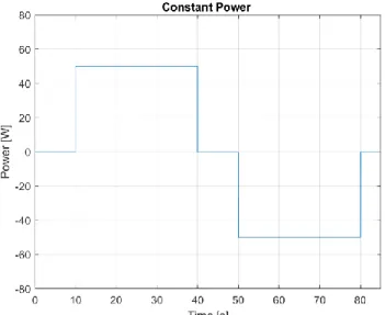
Before the injection there is zero power and so zero current. Then it started to be injected a constant power. The injected power is positive and the extracted one is negative as shown in Figure 1.10.

At the initial moment it is 𝑉₀ = 𝑉_𝑚𝑖𝑛 and it is possible to continue inserting power in the

supercapacitor till the maximum voltage. In the same way it is possible to pick out power from the supercapacitor until half the rated voltage. Figure 1.9 shows the voltage trend, starting from half the

rated voltage and increasing as long as current is injected.

1.3.2 Constant power

19

The voltage across the component ideally follow the below relation

𝑉 = √𝑉₀2±2𝑝

𝐶 (𝑡 − 𝑡0)

1.17

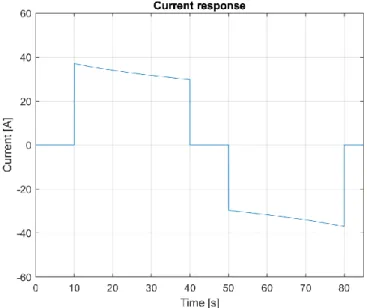
The positive for the charge, the negative during the discharge. Now the voltage is varying, and the power is constant. A constant power means that the current has to vary because the product of

Figure 1.10 Constant power injection and extraction

20

current and voltage must supply a constant quantity. This means that the current has to decrease to maintain the power constant. The current trend is shown in Figure 1.11. It can be seen that the voltage

varies with the square root of time and so the current decrease with the same trend, as shown in

Figure 1.11. When the maximum voltage is reached, the injection will no longer take place. And the

same goes for the minimum voltage. Once the extraction is reached, it must be blocked so as not to drop below the threshold (this is to allow the converter to adequately control the power exchanged).

It can be seen that by inserting and extracting power in the SC the voltage will increase and decrease. But being the power constant, it means that the current will vary because the product of current and voltage.

So, starting from the initial instant, the required power is zero therefore the current will also have a zero value. Then the charging phase starts then, the injected current starts from the value 𝑖 = 𝑝

𝑉𝑚𝑖𝑛 . At the beginning of the charge the voltage is equal to the minimum voltage value (nominal voltage) therefore the current will start from the value 𝑖 = 𝑝

𝑉𝑚𝑖𝑛 . During the charging phase then the voltage

21

will rise, and consequently the current will have to decrease to keep the power constant. Once the charging phase is over, the current will have a value of 𝑖 = 𝑝

𝑉𝑚𝑎𝑥 , a non-linear increase of the current from the initial to the final value is obtained. This is due to the fact that the voltage, grows with the square root of time (see Figure 1.12). The same thing happens for the discharge phase. The current

starts from a minimum value and then increases to the maximum value when the voltage is half the nominal.

This is the operation neglecting the serious resistance, but its effect cannot be overlooked. Now let's see the behavior considering also the series resistance.

In the same way we start with zero power and zero current. Once the power injection has started,

having the voltage at the minimum value (half of the rated voltage) we will have the maximum current. Here the voltage drop on the resistance will therefore be maximum, as shown in Figure 1.14.

22

As you can see, in the first case the voltage drop is just over 0.012V, while in the second case it is around 0.01V.

In Figure 1.13 can be observed that the voltage rises with the same trend until it reaches the maximum

voltage. Once the maximum value is reached, the power injection will stop and therefore the current will also stop. Here again I have a voltage drop which, however, will be less due to the fact that

Figure 1.13 Voltage response taking into account the ESR

Figure 1.14 ESR voltage drop difference: on the left the drop at minimum voltage is represented instead on the right that one at the maximum voltage

23

when the voltage is maximum the current is minimum therefore the voltage drop will be smaller than that experienced when the charging phase began.

Efficiency η (𝑅𝑠, 𝑖)

90%

80%

200A 300A 1000A 1500A Current

The performance trend shows that a reasonable operating regime for the cell is around 100W. For high powers the efficiency decreases, and the use of multiple cells must be considered.

24

2 Chapter 2: Modeling of Supercapacitor Cells

For modeling of a supercapacitors, we start by model of single cell. In the literature, there are two main types of cell models, i.e. the physics-based models and equivalent circuit model. The focus of this work is on the equivalent circuit models that are approximations voltage-current characteristic of the cell. These models do not necessarily reflect the chemical actions inside the cell, but their can replicate the cells response with high accuracy. The cell model should have the following

characteristics:

• Accurate enough to represent a real supercapacitor cell, in particular in transient behavior • Simple enough for real-time simulations.

• Suitable for the time scale of the study (seconds to minutes)

2.1 Equivalent-circuit Modeling of Supercapacitors

In this chapter, some of the most famous models of supercapacitors are introduced. The modeling of the component is addressed from different points of view, starting from the molecular aspect up to what concerns its most macroscopic behavior. The latter is the one on which the thesis will be focused and therefore models that develop the molecular aspect of the component will not be

considered.In literature, several models for supercapacitors are introduced, from which four models have been identified for the purpose of this work. These are

 The RC series model  The Two-Branch model  The Zubieta model  The Series model

25

Excluding the RC model which only gives a simplified representation of the component’s behavior, the other models are more accurate due to the fact that they present a breakdown of the time constant within a cell, dividing its representation into several branches. Note that the value of the capacitance of the models may in general depend on the voltage. This aspect is fundamental to a better

representation of the behavior of the supercapacitor cell. In fact, the capacitance value tends to vary as voltage varies.

The first model to be examined is the RC series model shown in Figure 2.1. This is the simplest

model,widely used for the approximate analysis of the cell behavior as in the previous chapter. The RC series model only introduce one time constant governing the dynamic of the cell which is simply given by the product of the resistance and the capacitance of the cell, i.e. = 𝑅 ∙ 𝐶

This model is used to have a general overview of the component's behavior. It should be noted that this model does not take into account the self-discharge phenomenon as there is only one resistance in the model. This is one of the disadvantages of this model. It also cannot accurately represent

2.1.1 The RC series model

26

charging and discharging cycles with accuracy. In the latter there are voltage variations increasing and decreasing of the voltage that cannot be adequately represented with this model. On the other hand, however, this model has a great advantage which is its simplicity [7].

This model is more complex than the previous one. In fact, the Two Branch model, shown in Figure

2.2, is a model in which a subdivision of the time constant takes place [8]. The circuit consists of

several branches in which the representation of the component dynamics is divided.

Note that the first branch is composed of a resistance and a variable capacitor. This capacitor is the sum of two terms: a constant one and a voltage dependent one. The capacitance of this branch is the main accumulation component while the resistance of this branch is the one that acts as Equivalent

Series Resistance (ESR). This branch is the one with the fastest dynamics. The second branch represents the medium-long term and is in the order of magnitude of minutes. The second branch does not contain variable terms. The third and final branch is that which represents the phenomenon

2.1.2 The Two-Branch model

27

of self-discharge. This term is actually relevant for the complete representation of the component. However, this model is used for representations of a generally shorter period and, as in the case in question, it will not be considered. In this work, wesimplify this model by eliminating the third branch andobtaining the model of Figure 2.3 .

Increasing capacitor as voltage increases means that the stored energy also increases.

The third model is the Zubieta model shown in Figure 2.4 [9]. This model is very similar to the

previous (Two-Branch model). In fact, also this model, we have a subdivision of the various

dynamics of the component through multiple branches and the first branch has a variable capacitor. In particular, it can be seen that the first branch is composed of a series resistor (R1), which

2.1.3 The Zubieta model

28

represents the ESR. In series with the resistance there is the main capacitor consisting of two terms (C10, k*V) just like for the Two-Branch model. The first term will be constant and the second will depend on the voltage across the capacitor. The two components are in parallel, so the two capacitor values are added together. This branch defines the behavior of the circuit in the first few seconds. The second branch is composed of a resistance and a series capacitor (R2, C2). This branch has a time constant in the order of a few minutes. The third branch consisting of resistance and capacitor (R3, C3) has a time constant of over tens of minutes. Finally, the last branch represents the

phenomenon of self-discharge. In this model the last branch is considered because, being a model with a greater distribution of the dynamics of the system for our purpose it should be made up of all

its branches. In fact, this model should represent the behavior of the supercapacitor in a span of 30 minutes.

The timing is therefore longer than the two-branch model which should be based on fewer minutes.

29

The series model is the most complex of the four taken into consideration. It is shown in Figure 2.5. It

is made up of a large amount of components, many of which are variable with time [10]. This makes it a heavy and difficult model to implement. Also, reliable and robust identification of parameters is very complex. The peculiarity of this model is linked to the first branch. In fact, here we find a large subdivision of the time constant through parallels of resistance and capacitor. Each block of a parallel of resistance and capacitor, we call a block. In this work, five blocks are used to get a good model accuracy. Remember that the first branch deals with the faster dynamics of the system. It can be noted that in the first branch only the series resistance (equivalent of the ESR of the component) is a constant parameter while all the others are variable parameters. In series with the above-mentioned resistance we find a capacitor which is the main storage component. This is composed of a fixed part and a variable part.

2.1.4 The Series model

30

The variable part of each capacitance is obtained multiplying the voltage by a constant (k). In each block, is inserted half the value of the total capacitance given by summing fix and variable part.

The lookup table is a component used in Simulink to have voltage dependent components. In the case in question, it is calculated from 0 to the rated voltage (2.7V) as shown in Figure 2.6.

An interpolation is also made for the resistance placed parallel to the capacitor of each block. The resistance value of each block descends with 1

𝑛𝑏𝑙𝑜𝑐𝑘 , in which 𝑛𝑏𝑙𝑜𝑐𝑘 is the number of the block, following Equation 2.1. In that equation can be seen how every block has a different resistance. The time constant of each block decreases for each subsequent block. This is in order to accurately represent the fast dynamics of the system.

The equation of the parallel resistance of the blocks follows. In the blocks the reference resistor value is scaled for every block. Note that it decreases with the square of the block number (n).

𝑅_𝑝𝑛 = 2 ∙ (𝑉) 𝑛2_𝜋2_𝐶(𝑉)

2.1

31

So, once the behavior of the first branch has been defined, we find three other branches: now there is a lot of similarity with the Zubieta model in that each branch defines a time constant. Each parameter has a constant value just like the previous model. The last branch takes into account the

32

2.2 Model Validation

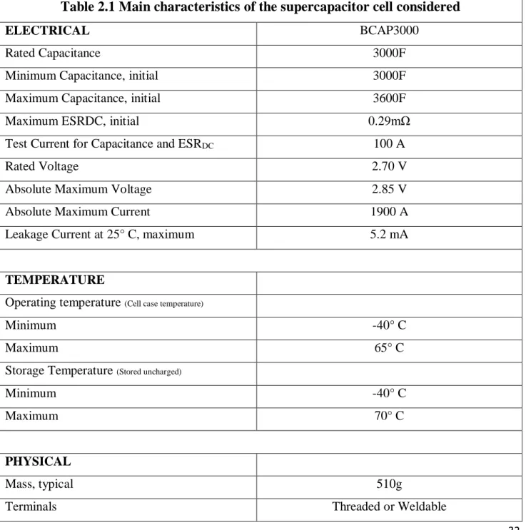
The supercapacitor cell that is considered for modeling is a Maxwell supercapacitor. All the cell data are shown below, directly from the data sheet provided by the manufacturer.

Table 2.1 Main characteristics of the supercapacitor cell considered

ELECTRICAL BCAP3000

Rated Capacitance 3000F

Minimum Capacitance, initial 3000F

Maximum Capacitance, initial 3600F

Maximum ESRDC, initial 0.29mΩ

Test Current for Capacitance and ESRDC 100 A

Rated Voltage 2.70 V

Absolute Maximum Voltage 2.85 V

Absolute Maximum Current 1900 A

Leakage Current at 25° C, maximum 5.2 mA

TEMPERATURE

Operating temperature (Cell case temperature)

Minimum -40° C

Maximum 65° C

Storage Temperature (Stored uncharged)

Minimum -40° C

Maximum 70° C

PHYSICAL

Mass, typical 510g

Terminals Threaded or Weldable

33

Maximum Terminal Torque (K04) 14 Nm

Vibration Specification ISO 16750, Table 14

Shock Specification SAE J2464

POWER & ENERGY BCAP3000

Usable Specific Power, Pd 5,900 W/kg

Impedance Match Specific Power, Pmax 12,000 W/kg

Specific Energy, Emax 6.0 Wh/kg

Stored Energy, Estored 3.04 Wh

SAFETY

Short Circuit Current, typical (Current possible with short circuit from rated voltage. Do not use as an operating current.)

9,300 A

Certifications UL810a, RoHS

TYPICAL CHARACTERISTICS

THERMAL CHARACTERISTICS

Thermal Resistance (Rca, Case to Ambient), typical8

3.2o C/W

Thermal Capacitance (Cth), typical 600 J/o C Maximum Continuous Current (ΔT = 15° C) 130 ARMS Maximum Continuous Current (ΔT = 40° C) 210 ARMS

LIFE

DC Life at High Temperature (held continuously at Rated Voltage and Maximum Operating Temperature)

1,500 hours Capacitance Change (% decrease from minimum initial

value)

20%

34

Projected DC Life at 25° C (held continuously at Rated Voltage)

10 years

Capacitance Change (% decrease from minimum initial value)

20% ESR Change (% increase from maximum initial value) 100%

Projected Cycle Life at 25°C 1000000cycles

Capacitance Change (% decrease from minimum initial value)

20%

LIFE

ESR Change (% increase from maximum initial value) 100%

Test Current 100A

Shelf Life (Stored uncharged at 25° C) 4 years

Table 2.1 Product specifications

Figure 2.7 shows the capacitance behavior as function of the temperature:

it can be noted that optimal operation can be obtained between about 0 ° C and an ambient

temperature of around 25 ° C. In this range it is possible to obtain the maximum capacitor and have an ESR that varies around the minimum value as shown in Figure 2.7. This is something that is

Figure 2.7 ESR and Capacitance as function of the temperature. Courtesy of picture: Maxwell Technologies

35

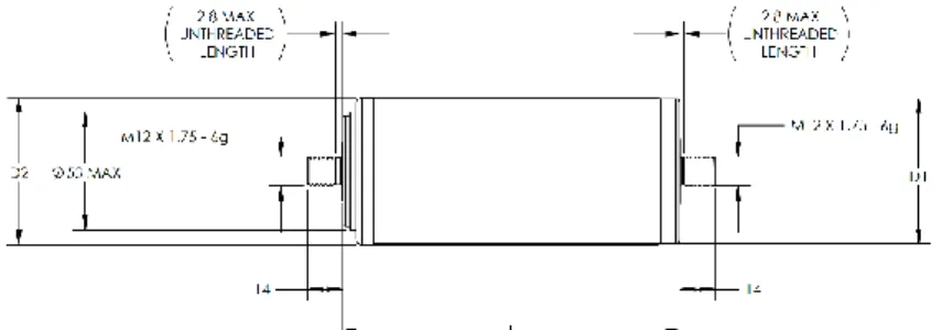
important from the point of view of performance as it is this resistance value that particularly influences it. The structure of the supercapacitor cell is described in Figure 2.8 and Figure 2.9.

Dimensions are shown in Table 2.2.

Dimensions (mm)

Part description L (±0.3mm) D1 (±0.2mm) D2 (±0.7mm) Package Quantity

BCAP3000 P270 K04/05 138 60.4 60.7 15

Table 2.2 Dimensions of the supercapacitor cell

Figure 2.9 Cell structure from data-sheet(2). Courtesy of picture: Maxwell Technologies

Figure 2.8 Cell structure from data-sheet. Courtesy of picture: Maxwell Technologies

36

Here, the experimental setup and procedure of the supercapacitor cell is explained. Two-quadrant operation of the supercapacitor has been made possible by:

 One-quadrant TDK Lambda GEN8 (400A – 8V), current source, and dump resistor  Power MOSFET inverters

 Labview management system

Feedback control of source current allowing the two important operation modes:  Constant current cycling

 Constant power cycling

2.2.2 Experimental Setup

37

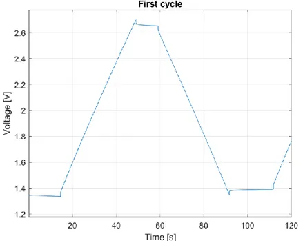
The component is tested by carrying out charging and discharging cycles at constant current on it. The start is from half of its rated voltage, so in this case it is 1.35V as shown in Figure 2.11. The test

will take place symmetrically with positive and negative current pulses in a periodic way (see Figure

2.12). The first cycle has an asymmetry due to ESR which causes an increase in voltage from the

second cycle onwards. This occurs because what controls the insertion of current into the component is its voltage level. By starting to inject a positive current, the charging phase of the first cycle will end when the rated voltage is reached (2.7V in the case under consideration). Once at nominal voltage the current value will go to zero. before the discharge phase there are 10s of waiting. Then the discharge phase begins, and the voltage begins to decrease. It is important to note that the sequence of moments in which ESR influences causes the initial voltage of each cycle following the first to be greater than the initial voltage at the instant t =0. There is a 20s off period before the next positive impulse. This process is repeated up to having four charge-discharge cycles. Thus we note that our component is kept cyclically charged for 10s. The voltage then decreases until it reaches half

38

the rated voltage where the current returns to 0.Four charge and discharge cycles are applied. There is a 20s off period before the new positive impulse. And so, on up to having four charge-discharge

cycles. Thus, we note that our component is kept cyclically charged for 10s. So what we get is the live response shown in Figure 2.13.

Figure 2.12 Input current pulses sequence.

39

Now, knowing the response of the component, we will proceed with the estimation of the parameters of the models that have been introduced. The supercapacitor models are (apart from the RC model) quite complex, in particular the series model. To obtain all the parameters of each model, the

MATLAB/Simulink parameter estimation tool was used to estimate the parameters. This tool allows, with the input and output data, to estimate each parameter of the circuit. The circuits are

implemented in MATLAB/Simulink. The experimental data are voltage and current values. These are inserted into the tool. In the toolbox it is also possible to define a range, so that the parameters can vary but in a limited way (i.e. within the range). Once the conditions in which the parameters will be estimation are set, the estimate is carried out. During the estimation it will be possible to monitor the execution of the model as, at each variation the model runs to verify the actual accuracy of the variation.

2.2.3 Parameter Estimation Procedure

40

We then proceed with the estimation of the parameters of each model. This process involves different computation times for each model depending on its complexity. What may also affect the starting conditions of the estimate. Obviously if the entered parameters from which the estimate is already close to the final values, the estimation process will be faster because it will require less iteration to arrive at the solution. In fact, the achievement of a correct estimation depends on the value of the parameters at the beginning of the estimate. The more complex the model, the more local optimums can be found during the estimation process. This can lead to an incorrect estimate of the parameters which therefore will not allow the model to respond better.

The first model analyzed is the RC model. It is the lightest cause made up of only two parameters.

Parameter Value

R 0.41407 mΩ

C 3139.3 F

Table 2.3 The estimated parameters for the RC model

2.2.4 Comparison between Models

41

It can be noted that the estimated parameters are not too different from those reported by the

manufacturer. Now, to verify the actual quality of the parameter estimation of the model, the output of the model will be compared with the measurement. The comparison is shown in Figure 2.16 In this

way it is possible to see if the model answers correctly.

What we can see in Figure 2.15 representing the voltage is that there is a clear mismatch between the two. We can therefore conclude that the model is too poor to provide a correct representation of the behavior of a supercapacitor. In fact, although at the beginning the trends are very close, the

difference increases with time.Figure 2.16 shows is the absolute error calculated through the following equation.

𝐸_𝑎𝑏𝑠 = 𝑉_{𝑠𝑖𝑚𝑢𝑙𝑎𝑡𝑒𝑑} − 𝑉_{𝑚𝑒𝑎𝑠𝑢𝑟𝑒𝑑} 2.2

The absolute error is shown in Figure 2.17

42

We then move on to a more specific point of view looking at the relative percentage error. The model clearly cannot represent the component. Now the following equation is used to calculate the relative percentage error.

𝐸𝑟% =𝑉si𝑚− 𝑉meas

𝑉_meas × 100

2.5

Subsequently the data are displayed from the probabilistic point of view in Figure 2.19. The error is

inserted into a fitting function, to find the probability density function of the error. In this way it is possible to see precisely the density for each error value, showing more clearly where the error is concentrated. For this model, note that the distribution range is quite wide: in fact, the error increases with time and

43

this determines a wide range and a lower density value for each relative percentage error value.

Figure 2.18 RC series model percentage relative error

44

The next model analyzed is the Two-Branch model. For the reasons already explained, the entire analysis process will be carried out with the simplified Two-Branch model.

There are five parameters that will be estimated in the model. The model is not yet excessively complex, therefore, starting from not too random values, the estimation procedure does not take a long time.

Parameter Estimate Standard Error

μ 2.06856 0.00210682

σ 1.29873 0.000148975

Table 2.4 Parameters of the distribution function of the RC series model

45

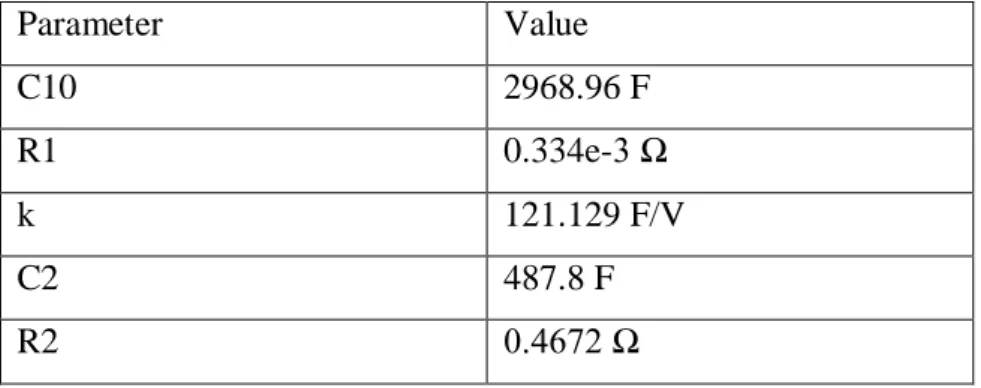
We can see from the estimated values that R1 is the parameter that represents what would be the series resistance of the component and C10 is the main capacitor of the model with a value really

Parameter Value C10 2968.96 F R1 0.334e-3 Ω k 121.129 F/V C2 487.8 F R2 0.4672 Ω

Table 2.5 Two-Branch model estimated parameters

46

close to what is declared by the manufacturer. It can be seen that the time constants of the two branches are different.

Figure 2.23 Peak of the second peak Figure 2.22 Second positive peak

47

Looking at the voltage response of the model, it can be seen that it is close to the measured value.

Figure 2.25 Two-Branch absolute error and percentage relative error Figure 2.24 Second negative peak

48

Leaving aside the first cycle for the above-mentioned reasons, one can better observe the critical points of the representation.

From Figure 2.26 it can be seen that the difference is minimal since the absolute error is around

0.005. To better see the accuracy of the model, after looking at the negative peak to see that there are no big differences between positive and negative, the errors are shown.In fact, we see that the error is minimal and acceptable. It is below 1% and has a periodical trend. This means that, in a longer test period

Parameters Estimate Standard Error

μ 0.0479518 0.00017131

σ 0.211205 0.000121135

Table 2.6 Parameters of the Two-Branch relative error density distyribution Figure 2.26 Two-Branch density distribution

49

there would be the possibility that this error always remains within a certain range. Which does not happen for the RC model for example, where an error increasing with time is observed. What is interesting to see is that the error is around 0. But this can be seen better by the density distribution function, where the density for each error value is highlighted.

The next model that will be analyzed is the Zubieta model, which is very similar to the previous one.

Parameter Value C10 2934.7 F R1 0.32232 mΩ k 130.81 C2 76.841 R2 0.38065 Ω C3 1518.8 R3 1.3284 Ω Rleak 59436 Ω

Table 2.7 Estimated parameters of the Zubieta model

The value of the main storage component is 2937.7 F, and it is close to the declared value in the data sheet. The value of R1 is also close to the value of the equivalent series resistance.

50

In this case all parameters are estimated for a total of eight. Again, we have the main capacitor C10 and a factor k that multiplies the voltage across it. As can be seen, the time constants of each branch are different, and vary from the fraction of a second to tens of minutes, covering a period of about

thirty minutes fairly evenly.The graph of the voltage across the model during its execution, however, the model accuracy is not better than the two-branch model. It can be seen that the error is

Figure 2.29 Percentage relative error of the Zubieta model

51

increasing. Error values are higher than the Two-Branch model although they are very similar. The error distribution is not centered in zero: this means that on average the error is not zero.

The last model analyzed is the Series Model. This, due to its complexity, requires some precautions in estimating the parameters. In the parameters estimation it results difficult to estimate many parameters cause of the risk of find local minimums. To avoid this, some parameters are set to reduce the number of estimated parameters. Particularly, to implement the model on

MATLAB/Simulink lookup tables are used.

Parameters Estimate Standard Error

μ 0.705316 0.000239882

σ 0.295746 0.000169622

Table 2.8 Parameters of the percentage relative error density distribution of the Zubieta model

52 Parameter Value R2 55.9 mΩ C2 95.11 F R3 676 mΩ C2 453.27 F Rleak 63186 Ω Rps 49799e-05 Ω C+k*V 3250F Ri 0.32232 mΩ

Table 2.9 Estimated parameters of the series model

The lookup-table receives as input a voltage value and two arrays: one with the voltage values and one with the resistance/capacitance value. The two arrays (Equation2.3/Equation2.5 and

Equation2.6)are used to do an interpolation of the value of resistance/capacitance as function of the voltage. So, once have received the input voltage, the lookup-table block gives as output the value of the variable component at that voltage.

So, setting the values of the coefficients and estimating the reference values of the arrays (Rps, Cest) for which they will be multiplied, we arrive at the implementation of the whole model. Table 2.10

contains fixed values used for the interpolation. Table 2.9 is instead containing reference values (Rps,

Cest), that have been estimated.

Resistance Capacitance

rp1(0V) rp2(1.35V) rp3(2.7V) cr1(0V) cr2(1.35V) cr3(2.7V)

0.965 0.97 0.98 0.88 0.92 0.95

53

𝐿𝑜𝑜𝑘𝑢𝑝 − 𝑡𝑎𝑏𝑙𝑒_{𝑟𝑒𝑠𝑖𝑠𝑡𝑜𝑟} = 𝑅𝑝𝑠 ∙ [𝑟𝑝₁ 𝑟𝑝₂ 𝑟𝑝₃] 2.3

𝐶_𝑒𝑠𝑡 = 𝐶 + 𝑘 ∙ 𝑉 2.4

𝐿𝑜𝑜𝑘𝑢𝑝 − 𝑡𝑎𝑏𝑙𝑒_{𝑐𝑎𝑝𝑎𝑐𝑖𝑡𝑜𝑟} = 𝐶_𝑒𝑠𝑡 ∙ [𝑐𝑟₁ 𝑐𝑟₂ 𝑐𝑟₃] 2.5

𝑉 = [0 1.35 2.7] 2.6

The condition of the starting voltage is 1.35V for all models (Figure 2.34). Figure 2.31 shows the

voltage response of the Series model.

54

Note that at a glance the behavior seems satisfactory (see Figure 2.32), even giving observing the

progress of the error it is. In fact, we can note that the error has a periodic trend, which means that the model has good stability. The percentage relative error tends to remain around 0 as shown in

Figure 2.33, so it could be defined as stable.

Figure 2.33 Percentage relative error of the series model

55

Parameter Estimate Standard Error μ -0.0240044 0.000796805 σ 0.490988 0.000563427

Table 2.11 Parameters of the density distribution of the percentage relative error of the Series model

To get an idea of which model is actually having the best performance it would be necessary to see their comparison. We start with the visualization of the voltages generated by each model. All the voltage responses are compared in Figure 2.34.They will be compared and analyzed in the critical

points.

In addition, the voltage measured experimentally is also showed, as a reference. It is interesting to see closely at the behavior of the model in the critical points, which in this case are mainly the voltage peaks. In fact, in them there is the greatest mismatch for each model.

56

Starting from the first voltage peak we note that the voltages are all very close apart from the voltage of the RC model which is already slightly higher. While Zubieta and Series models exhibit equal voltage as shown in Figure 2.35. The Two-Branch model is the closest to the experimentally

Figure 2.35 Detail of voltages in the first two peaks

57

measured voltage. Note that before the peak the voltage is rising when the voltage reaches 2.7V and therefore the injected current becomes zero, the series resistance contributes by slightly lowering the voltage value. It is important to note that the difference in amplitude that exists at this instant, i.e. after the voltage has been affected by the drop on the series resistance, is approximately the same as in the phase in which the voltage rose. So, this difference should not be associated with the abrupt variation because in fact it was present even before. In the second peak we can see how the voltage of the RC model moves away from the reference while that of the Two-Branch model goes slightly below the measured voltage. The Series and Two-Branch models are closest to the measured voltage, the Two-Branch model in particular. In the third peak in Figure 2.36 it is easy to see the voltage

simulated by the RC model at a clearly unacceptable value while the Series and Two-Branch models remain close to the experimental value.

58

A comparison between the relative errors of the models is also shown in Figure 2.37 to compare their

progress.

Figure 2.38 shows a comparison of the density distributions of all models.

The error of the RC model brings it shows that it is not suitable for representation.Its error grows over time and the density distribution with a wide range and low peak value highlight the

inappropriate use. The trend of the error of the Zubieta model instead indicates that the trend is unstable as the error tends to increase. The density distribution is not very close to 0 but is still quite concentrated. However, the fact that the error increases makes it unsatisfactory. So, it is not good for

59

the representation of the component. The remaining two models have already proved to be good enough for representation. The trend of their error is therefore also satisfactory. In fact, they are both periodic cycle after cycle remaining in a fairly small range and around 0. However, the range of the Two-Branch model is smaller, and its peak density is therefore considered the best of the two. The basis of the consideration is obviously the influence of the complexity factor of the model: in fact, the Series model is more difficult to implement, with many parameters. Also, from this point of view therefore the Two-Branch model would be preferable.

60

Model Parameter Estimate Standard Error

RC series model μ 2.06856 0.00210682 σ 1.29873 0.000148975 Two-Branch model μ 0.0479518 0.00017131 σ 0.211205 0.000121135 Zubieta model μ 0.705316 0.000239882 σ 0.295746 0.000169622 Series model μ -0.0240044 0.000796805 σ 0.490988 0.000563427

61

3 Chapter 3: Real-Time simulation of Supercapacitor

3.1 Real-Time simulation and its applications

In this chapter, the concept of real-time simulation is introduced, and a new tool to analysis and design of components and power systems is explained. In particular, we start with the introduction of DRTS (digital real-time simulation) as a tool for the representation of power systems in a real way, reproducing their behavior in real-time. The systems are first represented through particular software with user graphic interfaces and are then simulated in particular platforms. For real-time simulations time, in order to have a correct data acquisition it has to be

EXECUTION TIME (Te) ≤ TIME STEP (Ts)

The execution time is the sum of time needed for measurement, computation and command. This sum has to be smaller than the set step time. Otherwise, an overrun will occur and an increase of the time step will be necessary. Overrun is when the time of these three parts exceeds the given

simulation step. If this problem occurs, it is necessary to modify the simulation step time

Real-time simulations enable Hardware-in-the-Loop (HIL) testing, in which parts of the simulated system are replaced by physical components using input-output interfaces. Here the hardware under (HuT) test may be controllers that regulate switches or the connections and disconnections of some components. If controllers are tasted it is called CHIL (Control Hardware in the Loop). In these systems there are no real power flows and the whole system is modeled as something virtual that is inside the simulator.

62

[11]

When there is a real hardware under test, we talk of Power Hardware in the Loop (PHIL), as in Figure

3.1. In the PHIL there is a power interface that can both absorb and generate power, allowing

bi-directionally of the power flow. So, in PHIL it presents a power transfer to or from the Hardware under Test (HuT). Both in CHIL and PHIL is present the human machine interface (HMI). There is a simulated system part and an externally connected part. The power source can supply or generate power. Then, the system is solved and the signals that are generated go to the HuT. First, they are sent to an amplifier that supplies voltage or current to be applied to the HuT.

The first simulators were based on a digital signal processor. There was an expansion of general-purpose processors because they were cheap, and their development cycle was fast. RTDS Technologies Inc. launched the first digital real-time simulator on the market in 1991[11]. It has combined analog and digital parts. The OPAL-RT Technologies Inc. simulator was introduced around the year 2000. ARENE (from Électricitè de France), NEOTOMAC (from Siemens) were

Figure 3.1 Controller Loop (CHIL) and Power Hardware-in-the-Loop (PHIL).

63

introduced in the same years. OPAL-RT is the only one using MATLAB / Simulink as a simulation modeling tool.

A real-time simulator must be able to solve the model under 50μs, this in order to have a good accuracy of power system phenomena. If instead one needs analyze something faster like a microcontroller where there are higher frequencies, the time can be around 1μs or even 10ns.

However, it can happen that there are very fast internal dynamics, but it is not necessary to use a very

small time-step. Figure 3.2 ([11]) shows the relationship between computing nodes and time-step

requirements for different systems. The simulation of the power system simulation can be carried out with comparatively larger time-step, and for a constant computing power, it allows a larger system, whereas for power electronics simulation, smaller time-steps are necessary, resulting in a smaller system for the same computation power. It is possible to increase the calculation power of the simulator as the parallel operation unit, but a delay for communication is added. Communication is

64

optimized by exploiting the properties of the transmission lines separate the network subsystems with an adequate length, consistent with the simulation steps.

Most simulators have the following characteristics:

 multiple processors working in parallel that form the platform where the real-time simulation is performed

 an external computer on which the model previously created offline, built online, uploaded and executed (using the same computer to monitor the simulation)

 input-output terminals for the hardware interface

 a communication network in case the model is divided into several subsystems

An example of hardware of type A is shown in Figure 3.3.

65

Now we move on to a hardware description starting with the description of type A [11]. This is made up of various units called racks that contain various processor boards. Each processor board contains two processors that work in parallel. They make up the main calculation engine. Each rack is

therefore made up of twelve processors or six boards. The maximum number of nodes of the power network that can be simulated is 72. There is a network solution for each processor. Each simulator also contains a workstation network interface: this allows communication and synchronization with real-time operation of the components. Through the use of some cards it is possible to switch to a synchronization that can also facilitate the connection with the outside. By combining processors, more effective results were also obtained.

The type B simulators ( architecture shown in Figure 3.4 [11]) have undergone rapid development of

communication techniques and protocols for sharing. All this thanks to the rapid development of network and communication technologies. Type B is the multi-CPU simulator. This can be extended to multicore with each core modeling a subsystem. The shows how the various hardware components

66

are connected. There are reconfigurable FPGA (field programmable gate array). The input-output signals are conditioned by these FPGAs. This type of simulator, which can also use different

toolboxes, personalizes the system by orienting itself towards the integration of FPGA components, graphics processing unit (GPUs) or in any case sets of hardware components.

The type B is of interest for this work. Particularly Figure 3.4 shows the structure of the simulated

used in this analysis. In fact, eMEGASIM is the software used. It is compatible with Simulink and Simscape Power Systems MATLAB tools.

From the point of view of software, simulators can generally request two categories of software: operating system or application software. In general, the simulators work both on Windows and on Linux operating system, however, if necessary, in some cases particular operating systems may be necessary. Generally, in these cases the systems are supplied together with the hardware. Software applications in general can have particular interfaces and system configuration platforms in which the model can be adapted so that it is correctly read by the simulator and executed.

As for the interface and communication, type A connections are available for all racks to facilitate communication. In addition, fiber optic connections are used. In the event that there are more than seven racks, an inter rack communication is carried out with a point-to-point methodology. All this using Ethernet. On the other hand, for types B, thanks to the rapid technological advancement, there are various communication techniques and protocols used for the transfer of information. These include inter CPU communication signal wire, InfiniBand and others.

The modeling tools for type A simulators are available GUI libraries as an integral part that allow the construction of power system models with the necessary controls and protections. As far as the time-step is concerned, there is a time between 1-4 microseconds, therefore small, for the subsystems but