Non-Linear Analysis and Design of Cable Systems in Suspension Bridges

ALMA MATER STUDIORUM - UNIVERSITÀ DI BOLOGNA

SCUOLA DI INGEGNERIA E ARCHITETTURA

DIPARTIMENTO DI INGEGNERIA CIVILE, CHIMICA, AMBIENTALE E DEI MATERIALI

CORSO DI LAUREA IN CIVIL ENGINEERING

TESI DI LAUREA in

Advanced Design of Structures

Non-Linear Analysis and Design of Cable Systems in Suspension Bridges

Anno Accademico 2016/2017

Sessione III

CANDIDATO: RELATORE:

Riccardo Soli Prof. Stefano Silvestri

CORRELATORE: Prof. Peter Ansourian

Summary

The scope of the presented research project is to provide a reliable guideline for the preliminary design of cable supported bridges. In order to pursue this objective, a thorough literature research has been conducted in the first phase of the project. This has been of relevant importance for the understanding of the subject and further implementation of the case study: the design of a suspension bridge model in Strand7.

The conducted research has shown that there is not a unique book to which engineers may refer in order to conduct the type of analysis presented in this project. Therefore, the proposed guideline has been created on the basis of multiple text books.

Further analyses have been conducted in order to evaluate the accuracy of theoretical-based results and software-based results. In particular the Steinman Modified Elastic Treatment has been applied to the case study and its results compared to those obtained on Strand7. The obtained results finally show that Steinman’s Theory represents a quick and reliable method to be adopted for preliminary design purposes as its results are in line with Strand7 results.

Index

1. Introduction 1

2. Literature Review 3

2.1. Structural Behaviour of Cables 3

2.1.1. Catenary Curve 3

2.1.2. Parabolic Curve 4

2.1.3. Cable with Inclined Chord 5

2.1.4. Comparison of Cable Shapes 6

2.1.5. Final Considerations 8

2.2. Structural Behaviour of Cables under Applied Loads 9

2.2.1. Single Concentrated Load 9

2.2.2. A Short Distributed Load Centrally Placed 12 2.2.3. A Short Distributed Load at One End of the Span 13

2.2.4. Final Considerations 14

2.3. Analysis of the Theories for Suspension Bridges 15

2.3.1. The Rankine Theory (1858) 15

2.3.2. The Elastic Theory (19th century) 18

2.3.3. The Deflection Theory (1888) 21

2.3.4. Final Considerations 23

3. Case Study: Modelling a Suspension Bridge on Strand7 25

3.1. Materials 25

3.1.1. Girder and Pylons 25

3.1.2. Cables and Hangers 25

3.1.3. Concrete Deck 26

3.2. Defining Span Proportions and Lengths 26

3.3. Truss Girder 27

3.4. Hangers 30

3.5. Cables’ Profile Definition and Preliminary Design 33

3.5.1. Catenary VS Parabola 33

3.5.2. Main Suspension Cable 36

3.5.3. Side Suspension Cables 40

3.6. Pylons 47

3.7. Strand7 Simulation 48

3.7.2. Linear Static Analysis 49

3.7.3. Non-Linear Static Analysis 50

3.8. Comparing Steinman’s Solution with Software-Based Results 53 3.8.1. Steinman’s Modified Elastic Treatment 53

3.8.2. Strand7 Solution 61

3.8.3. Analysis of Results 63

3.8.4. Final Considerations 65

3.9. The Influence of Side Spans 66

3.9.1. Long Side Spans Suspension Bridge - Design Parameters 67 3.9.2. Strand7 Simulation - Non-Linear Analysis 70 3.9.3. Comparing Long Span and Short Span Suspension Bridges 71

4. Conclusions 73

5. Acknowledgments 75

References 77

1. Introduction

Cable supported bridges are generally subdivided in two main categories depending on the asset of their cable system:

• Suspension Bridges, where the stiffening girder is connected to the main parabolic cables by means of vertical or inclined hangers;

• Cable-Stayed Bridges, where the stiffening girder is directly connected to the pylons by means of straight or quasi-straight cables.

The two typologies are shown in Figure 1.1 below.

Figure 1.1: Golden Gate Bridge (San Francisco, US) and Millau Viaduct (Creissels, France).

The linearity of the problem comes from the sag of the cables which provokes a non-constant tension along the cables’ length. It is generally simpler to identify the sag in suspension bridges and more difficult in cable-stayed bridges due to different sag ratios adopted in practice. However, Figure 1.2 below shows the presence of sag in cable-stayed bridges:

!

The conducted research is aimed to the determination of preliminary design guidelines for cable supported bridges, with a particular focus on suspension bridges. The common literature shows that the behaviour of stay cables can be generally approximated and related to that of straight cables with the adoption of some precautions. This has led to a greater personal interest in the behaviour of suspension bridges and it is therefore the reason why the case study reported in Chapter 3 refers to this type of structure.

First step of this project is the analysis of the main theories developed through history for cable supported bridges (Chapter 2), in order to gain the proper knowledge required for the implementation of the case study. As it is explained in Chapter 2, the ongoing development of the theories for cable supported bridges has led to numerical solutions that were once hard to be applied by structural engineers, who did not have the availability of softwares like Strand7 as we do today. Simplified theories were thus developed for practical purposes and this research will investigate the accuracy of one of these by comparing its results with those obtained on Strand7.

Chapter 3 reports the case study: the preliminary design of a suspension bridge and the creation of the Strand7 model to be adopted for further analyses. The reported guideline is the result of a research conducted on different text books and can be also applied to suspension bridges having different geometric characteristics to those adopted in this study. The design guidelines are particularly focussed on the cable system whilst the bridge’s girder has been modelled on Strand7 according to common practice knowledge.

Moreover, Chapter 3 includes a comparison between the results obtained on Strand7 and those given by the application of the Steinman’s Modified Elastic Treatment to the case study. The obtained results prove the reliability of Steinman’s Theory and therefore make it a reliable tool to be adopted for the evaluation of the effect of Live Loads on the cable system.

Finally, an analysis of the effect of the side spans’ length on the design of the suspension bridge has been conducted by the creation of a second model on Strand7.

2. Literature Review

2.1. Structural Behaviour of Cables

The non-linearity of cable systems due to the change in sag and axial tension represents a fundamental problem in the analysis of cable structures. Therefore the first thing that has to be analysed is the shape that a freely suspended cable would take when loaded by its own weight.

For obvious reasons the complete calculations for the determination of the cable’s shape and tensions are not reported, as they can easily be found in many books and to which the following paragraphs are referred. The catenary problem was solved by J. Bernoulli at the end of the seventeenth century, whilst the solution to the parabolic curve was first proposed by N. Fuss at the end of the eighteenth century. Both solutions are collected in “The Theory of Suspension Bridges” (Pugsley 1968), and presented below.

2.1.1. Catenary Curve

The cable is assumed to be:

• Perfectly flexible: the cable carries any load by means of tension directed along its length; • Inextensible;

• Uniform: weight per unit length (! ) is constant along the cable.

Under these assumptions, the shape that the cable takes when suspended between two fixed nodes is known as “catenary”.

!

Figure 2.1: Catenary Curve (Pugsley 1968).

This problem has been solved by starting from Equilibrium equations:

!

where T is the tension at any point of the cable, and H is the tension in the cable at point C. ′ w (1) T cos

( )

( )

As outputs it is possible to obtain the “Cartesian Equation of the Catenary”:

!

where “c” is the “parameter of the catenary”, which can be obtained by using tables of hyperbolic functions.

Moreover, the tension in the cable is expressed by the following:

!

and its horizontal component is expressed as:

!

The following observation can be made upon the obtained results:

• The horizontal component of the cable’s tension, shown in equation 4, is constant; • The vertical component of the cable’s tension is expressed at any point of the cable as:

!

2.1.2. Parabolic Curve

The cable is assumed to be:

• Perfectly flexible: the cable carries any load by means of tension directed along its length; • Inextensible.

The third assumption though is different from the one considered in the catenary formulation, as it refers to a practical situation in which the total dead weight of the structure is uniformly distributed along the span of the bridge, not along the cable. Therefore the third assumption is: • Weight per unit length (! ) is uniformly distributed along the span.

!

Figure 2.2: Parabolic Curve (Pugsley 1968).

This problem has been solved by starting from Equilibrium equations: (2) y= c⋅cosh x c ⎛ ⎝⎜ ⎞ ⎠⎟ (3) T = ′w ⋅ y (4) H = ′w ⋅ s⋅cot⎡⎣

( )

!

where T is the tension at any point of the cable, and H is the tension in the cable at point C. The “Cartesian Equation of the Parabolic Cable” obtained is:

!

For the practical case of parabolic cable freely suspended between two nodes A and B at the same level, the tension in the cable T can be expressed as:

!

with horizontal component H equal to:

!

A useful result that this analysis provides in practical terms is the length of the sagging cable “l”. Assuming small ratios of d/L this length can be expressed as:

!

2.1.3. Cable with Inclined Chord

This study case is particularly useful for the analysis of cable-stayed bridges and the side span cables of suspension bridges. The complete calculations for this case are reported in “Statically Indeterminate Structures” (Maugh 1964) but for practical reasons only the main results are listed in this review, and were taken from “Construction and Design of Cable Stayed Bridges” (Walter Podolny 1976). When considering the condition represented in Figure A2.1 (reported in the Appendix), the relevant results are:

• Horizontal component of cable stress (H):

!

• Maximum tension stress in the cable (Tmax):

(6) T cos

( )

( )

!

• Vertical components of cable stress:

!

• Cable length:

!

• Cable elongation due to cable tension stress:

!

• Sagging cable’s (y) coordinates from the inclined chord:

!

It must be noted that in the practical analysis of cable-stayed bridges the inclined cable is usually assumed as a straight line. Podolny investigated the percentage error of cable tension due to this approximation and provided the results plotted in Figure A2.2 (reported in the Appendix) (Walter Podolny 1976). As it can be noticed from the plot, when the sag ratio is in the range 1:30 - 1:100, the error varies from 4% to 12% depending on the chord inclination.

2.1.4. Comparison of Cable Shapes

After the study of the two shapes that have just been analysed, D. Gilbert developed some calculations for the case of “The Catenary of Uniform Strength”, in which he investigated how cables having sectional area varying proportionally to their tension would behave. However, since the cables usually adopted in practice for the construction of suspension bridges have a uniform cross-sectional area, the results of this analysis will not be reported (Pugsley 1968).

Now that the two shapes that a cable would take under its own weight are known, it must be understood which model should be chosen for practical interest. Theoretically, the weight per unit length of a freely suspended cable would be constant along its length, therefore suggesting that the catenary curve is the most precise representation of a cable’s shape.

(12) T_max = H 1+ h L+ 4n ⎛ ⎝⎜ ⎞ ⎠⎟ 2 ⎡ ⎣ ⎢ ⎢ ⎤ ⎦ ⎥ ⎥ 1/2 (13) V_r = Hh L + wL 2 (14) S! Lsecϑ ⋅ 1+ 8n2 3sec4ϑ ⎛ ⎝ ⎜ ⎞ ⎠ ⎟ (15) ΔS ! HL AEsecϑ ⋅ 1+ 16n2 3sec4ϑ ⎛ ⎝ ⎜ ⎞ ⎠ ⎟ (16) y=4f′ L2 Lx− x 2

(

)

However, in practice, the stiffening girder on which the roadway is constructed is so hung to the cables by means of suspension rods that when the structure is completed and the temporary sustaining platforms removed, the cables will take a parabolic shape. It can therefore be stated that for practical purposes a parabolic form of the cable could be considered.

Support to this statement was not only given in Sir A. Pugsley’s book “The Theory of Suspension Bridges”, but can be also found in “Construction and Design of Cable Stayed Bridges”, a work by W. Podolny and J.B. Scalzi published in 1976 (Pugsley 1968; Walter Podolny 1976).

A logarithmic plot of the catenary and parabolic curves based on the sag ratio (n):

! and !

shows that the catenary curve and the parabolic curve diverge at a sag ratio of 0.15 (Walter Podolny 1976):

!

Figure 2.3: Catenary versus parabola (Walter Podolny 1976).

where (f) and (a) are defined in Figure A2.3 (reported in the Appendix) (Walter Podolny 1976).

Thus it can be stated that for sag ratios smaller or equal to 0.15, the approximation of the catenary curve with a parabolic curve represents a reasonable choice (Pugsley, 1968).

However, a practical example will be analysed in chapter 3 in order to determine the accuracy of the reported results.

2.1.5. Final Considerations

The analysis of the proposed results suggests that a parabolic curve can be adopted in future analysis as the sag ratios usually adopted in practice are comparable to 0.15.

It must be noted that the assumption of “inextensible cable” was considered in both the catenary and parabolic curve solutions (paragraphs 2.1.1 and 2.1.2). This assumption of course simplifies the analysis of cable structures but does not accurately represents reality. The first solution to the “Elastic Catenary” problem was given by Routh in 1891 (Routh 1891) but the result was too difficult to be applied in practical cases.

However, a simpler solution based on the parabolic curve was provided by Rankine in 1858 (Rankine 1858). Assuming that

• The cable is extensible; • The span L remains constant;

the change of dip ! can be calculated from the following system:

!

Once again this result is based on the assumption of constant span (L), which can not be ensured in practical cases as it depends from the bridge’s pylons. During the design phase, further considerations will thus have to be made to account for certain effects due to simplifications.

The second assumption on which we may focus is the one that considers the cable as “perfectly flexible”, thus neglecting the flexural rigidity that a real cable would have. An interesting analysis regarding the influence of flexural rigidity was conducted by H.M. Irvine and reported in his book “Cable Structures”. In particular, the following expression for the dip of a cable’s profile below the inclined chord is provided:

!

where (z) and (x) are the non-dimensional coordinates as shown in Figure A2.4 (reported in the Appendix). The parameter (! ):

Δd (19) Δl =16⋅ d 15⋅l 5− 24 d L ⎛ ⎝⎜ ⎞ ⎠⎟ 2 ⎡ ⎣ ⎢ ⎢ ⎤ ⎦ ⎥ ⎥Δd Δl = H⋅l AE 1+ 16 3 d L ⎛ ⎝⎜ ⎞ ⎠⎟ 2 ⎡ ⎣ ⎢ ⎢ ⎤ ⎦ ⎥ ⎥ ⎧ ⎨ ⎪ ⎪ ⎪ ⎩ ⎪ ⎪ ⎪ (20) z= x 1

( )

γ2 1+ tanh γ2sinhγ x − coshγ x ⎛

⎝⎜

⎞ ⎠⎟ γ

!

represents the relative contribution to the cable’s behaviour as if it were treated as a perfectly flexible cable or as a beam element. As it is explained in Irvine’s analysis, the value of ! is usually large for the majority of cable problems (order of 103_{) and therefore the effect of} flexural rigidity can be neglected. However, when concentrated loads are applied to the cable and rapid changes in curvature are unavoidable, the effect of flexural rigidity increases (Irvine 1981).

2.2. Structural Behaviour of Cables under Applied Loads

Once that the shape of a freely suspended cable is known, further analysis of the deformed shape that it would assume under applied loads can be conducted. The capability of a cable to resist deformation by means of its own weight is of fundamental interest in the analysis of suspension bridges. Rankine payed particular attention to this aspect in the Theory he published in 1858 (Rankine 1858), and the results presented in the following paragraphs were also inspired to some unsigned articles in the “Civil Engineering and Architects’ Journal” for November and December 1860 (Pugsley 1968). As for the previous paragraph, calculation won't be reported but reference will be made to relevant assumptions and results (Pugsley 1968).

2.2.1. Single Concentrated Load

Assumptions:

• Nodes A and B are positioned at the same level;

• The cable is subject to a load (! ) which is uniformly distributed along the span L, and includes the self-weight;

• Cable hangs in a parabolic shape (of which point C is the vertex); • The cable is inextensible.

!

Figure 2.4: Parabolic cable under the action of a concentrated load (Pugsley 1968). (21) γ = H⋅l2

EI

γ

In the undeformed configuration the equations expressing the parabolic shape and the tension (H) in the cable at point (C) are:

! ; !

as already reported in paragraph 2.1.2., by formulas (7) and (9).

When a force P is applied at Q, the vertex of the parabolic cable will shift to its new position (C’), and the tension at this point will be:

!

where (h) is the tension increment due to P.

The equation used to express the shape of the portion (A-Q’) of the cable will therefore be:

!

where the parameters ! and ! are referring to the new vertex (C’). The position of this new vertex is obtained by the equilibrium equations of the vertical forces and bending moment. In particular, the coordinates ! and ! of point (C’) measured from the initial vertex (C) are:

!

where (r = x/L) is also used to determine how the concentrated load is shared by the vertical reactions:

!

In order to define the tension increment due to P (h) a further assumption has to be made: • The extension of the cable due to (h) is negligible.

The result provided therefore is:

!

Further interesting considerations regarding the case of “Single Concentrated Load” are presented in (Pugsley 1968): (1) y= 1 2 w H ⋅ x 2 _{(2) H =} wL2 8d (3) H

(

)

(

)

(

)

(

)

( )

A. Vertical Deflections Under Concentrated Load

The relation expressing the vertical deflection at the loaded point (Q), where (x=rL), is:

!

where (r) represents the distance between the point (Q) where the force is applied and the parabola’s vertex (C) . A plot of the deflection (! ) for different values of (r) and (P/wL) is also provided in Figure A2.5 (reported in the Appendix).

Based on the results of Figure A2.5, a relevant consideration can be made: as the value of (P) increases the cable becomes stiffer. However, if it is assumed that the values of (P/wL) are small, formula (8) can be approximated and linearised as it follows:

!

By differentiating formula (9) it can be noted that that the maximum deflection is obtained for:

!

This means that the maximum deflection is obtained when the concentrated load (P) is applied at a distance of (0.29L) from the centre of the span, and it is equal to:

!

If it is assumed that the concentrated load is applied at the centre of the span (r=0), the deflection will be:

!

B. Influence Coefficients for Deflection

The author (Sir A. Pugsley) provides a table of flexibility coefficients for vertical deflections due to vertical concentrated loads. For the purpose of this analysis the cable was subdivided by means of nine points equally distributed along the span. By considering the following assumptions (Pugsley 1968):

• The concentrated load is small compared to the weight of the cable and deck (P/wL=0.1) • The principle of superposition applies

• The ratio d/L (dip to span) is small (0.1 approximately) (8) υ_Q = − P wL⋅ d ⋅ 1+12r2

(

)

( )

( )

(

)

( )

and by making use of formula (9), a set of flexibility coefficients can be calculated.

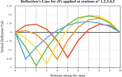
These flexibility coefficients are reported in Figure A2.6 (in the Appendix) and used to plot the influence lines for the analysis of cable’s deflection subject to a system of concentrated loads. In Figure 2.5 below, a plot of the influence lines for concentrated loads applied to stations 1 (in blue colour) to 5 (in red colour) are reported (the data were plotted using Excel):

!

Figure 2.5: Deflection’s lines for P applied at station points 1 to 5.

The horizontal origin axis represents the initial parabolic shape. The peak value for a given station (i) is of course obtained when the load (P) is applied at station (i). The maximum vertical downward deflection is obtained when (P) is applied at station 2 (green line).

2.2.2. A Short Distributed Load Centrally Placed

The assumptions to be considered are the same as those already reported in paragraph (2.2.1). The distributed load (p) is applied on a length of [(1-2n)L], and the self weight (w) is considered as well.

!

Under these conditions the following results are obtained (Pugsley 1968): • Vertical reactions:

!

• Equation of the parabolic arch AD (same shape assumed by arch EB):

!

• Equation of the parabolic arch DE:

!

• Final dip (D) at the centre of the span, expressed as a function of the initial dip (d) due to self weight only:

!

• The tension in the cable for (x=L/2):

!

2.2.3. A Short Distributed Load at One End of the Span

The assumptions to be considered are the same as those already reported in paragraph (2.2.1). In this case the distributed load (p) is applied at one end of the span as shown in the following figure (Pugsley 1968):

!

Figure 2.7: Parabolic cable under the action of a load (p) placed at one end of the span (Pugsley 1968).

Under these conditions the following results are obtained: (13) V_A= V_B = wL 2 + 1− 2n

(

)

(

)

(

)

(

)

( )

(

)

(

)

(

)

• Equation of the parabolic arch AQ, subject to the distributed loads (w) and (p):

!

• Equation of the parabolic arch QB, subject to the distributed load (w):

!

• The tension in the cable at the centre of the span:

!

In this case it will result more interesting to investigate the change of dip at a point F (as shown in the previous figure), rather than at the centre of the span, as it will become the lowest point under the action of (w) and (p). In particular, let xF and yF be the coordinates of point F:

-

-

By substituting (21) in (19) or (22) in (18), the change of dip at point F can be obtained.

2.2.4. Final Considerations

As it can be noted from the results presented in the previous paragraphs, the cable’s flexural rigidity is not taken into account. It is therefore interesting to understand how this aspect could affect the analysis of cable structures. As we will see in the following paragraphs, the effect of the flexural rigidity has been simplified in the earlier theories for the analysis of suspension bridges, and has only been considered at later stages.

(18) y=4d L2⋅ p w+1 ⎛ ⎝⎜ ⎞ ⎠⎟x L

(

)

( )

(

)

(

)

(

)

(

)

(

)

(

)

(

)

(

)

(

)

1+ p

wn 2

( )

(

)

2.3. Analysis of the Theories for Suspension Bridges

A brief analysis of the main theories that were developed for suspension bridges will be conducted in this chapter. The focus will be on the main assumptions on which these theories are based, on the obtained results, their evolution and limitations.

2.3.1. The Rankine Theory (1858)

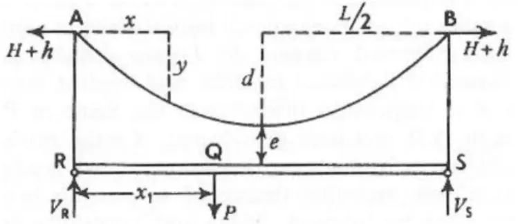
This is considered as the first proper theory of suspension bridges and was firstly published in 1858 by W.J.M. Rankine in “A manual of Applied Mechanics” (Rankine 1858). The proposed theory has also been included in other textbooks such as “The Analysis of Engineering Structures” (A. J. S. Pippard 1968) and “The Theory of Suspension Bridges” (Pugsley 1968). Rankine’s purpose was to demonstrate that there was no need to construct girders so stiff that they could bear their own weight, otherwise the role of the cable would have been pointless. The considered scheme will be the following:

!

Figure 2.8: Single span scheme (Pugsley 1968).

where points A, B, R and S are fixed.

• Assumptions on which the Rankine’s Theory is based

1. The cable takes a parabolic shape under the action of the total dead load on the bridge, and the stiffening girder would be unstressed

2. The stiffening girder redistributes any live loading so that the cable will be subject to a uniformly distributed load along its span;

3. The uniformly distributed upward pull that the cable is transmitting to the stiffening girder, is equal to the total live load divided by the span (L).

Assumption 2 is implicitly stating that the girder’s stiffness is relatively high.

The results reported in the following paragraphs were obtained by means of equilibrium only, with no regard to the displacement’s compatibility (A. J. S. Pippard 1968; Pugsley 1968).

A. Two-pinned Stiffening Girder with a Single Concentrated Load A load P is applied at a point Q, the upward pull (q) will therefore be:

!

By applying equilibrium the vertical reactions can be found:

!

The Bending Moment (B.M.) and Shear Force’s (S.F.) diagrams are provided in Figure A2.7 (reported in the Appendix). For the Bending Moment diagram, the upward pull (q) will result in a parabolic curved diagram, whilst the concentrated load (P) results in a triangular diagram. The obtained values are:

• Maximum value of the bending moment: !

• When (P) is applied at midspan: !

The increase in the horizontal component of the tension in the cable is:

!

and due to Assumption 3 the value of (h) is constant and does not depend on the point of application of the force (P).

It is also interesting to show how the bending moment (4) and the cable’s horizontal component of the tension (5) would change when considering a simply supported girder in absence of the cable, and a cable in absence of the girder. For a concentrated load (P) applied at midspan the following results can be compared:

Rankine also plotted the influence lines for bending moment and shear force in the stiffening girder, reported in Figure A2.8 (in the Appendix).

(1) q= P L (2) V_R = −V_S = P L L 2 − x ⎛ ⎝⎜ ⎞ ⎠⎟ (3) M_Q = −Px L

(

)

Suspension Bridge Girder Effect of the Cable

MQ

The presence of the cable therefore halves the B.M. at

midspan !−PL

4 !−PL

8

Suspension Bridge Cable Effect of the Girder

h The presence of the girder

reduces (h) by 50% !3PL

16d !PL

B. Two-pinned Stiffening Girder with a Uniform Load

By referring to the previous figure showing the influence lines for a concentrated load, it can be deducted that the maximum bending moment on the girder will occur for a load (p) of length (L/2) placed on top of the negative triangle. In particular, this bending moment can be calculated as the area of that triangle as (Pugsley 1968):

!

The maximum value of the bending moment is obtained for (! ), thus when point (Z) corresponds to point (C):

!

This value can be compared to the bending moment value in the girder in case that the cable was absent:

The effect of the cable would suggest that the required bending strength of the girder should be one quarter (1/4) of the one that a simply supported beam would have under the same applied load. Further calculations where done by Rankine for different load distributions and these led to the following result: the girder of a suspension bridge should have a bending strength which is approximately seven times smaller than that of a simple beam in order to carry the same loading (Pugsley 1968).

C. Three-pinned Stiffening Girder with a Single Concentrated Load

In this case the insertion of the central hinge has three main effects, that have to be compared to the results reported in case “A. Two-pinned Stiffening Girder with a Single Concentrated Load”:

• The upward pull is now a function of (x):

!

• The horizontal component of tension in the cable will therefore be: (6) M_Z = −1 8pL 2

( )

Suspension Bridge Girder Effect of the Cable

MC

The presence of the cable reduces the B.M. at midspan to a quarter of the value that a simply supported beam would have − pL2 8 − pL2 32 (8) q= 4Px L2

!

• A greater part of the applied load is carried by the cable. In fact the value of (h) when (P) is applied at the centre of the span is:

!

which is twice the value that was obtained for the two-pinned girder.

D. Three-pinned Stiffening Girder with a Uniform Load

In this case the insertion of the central hinge has one main effect, that have to be compared to the results reported in case “B. Two-pinned Stiffening Girder with a Uniform Load”:

• The critical length to be loaded in order to obtain the maximum bending moment is smaller (! ) and its value is approximately 40% smaller.

2.3.2. The Elastic Theory (19th century)

This theory was developed throughout the nineteenth century thanks to the application of the “Theory of Arches” by Navier (Résumé des Leçons données à l’Ecole des Ponds et Chaussées, 1826) and to later works conducted by Castigliano (Castigliano 1879). The well known “The Analysis of Engineering Structures” (A. J. S. Pippard 1968) was the first English book reporting this theory.

• Assumptions on which the Elastic Theory is based

The firs two assumptions are the same as those proposed in Rankine’s Theory:

1. The cable takes a parabolic shape under the action of the total dead load on the bridge; 2. The stiffening girder is unstressed;

The element of innovation stands in the third assumption:

3. The uniformly distributed load (q) acting on the cable mainly depends on four elements:

I. Girder’s stiffness (in bending) II. Cables’ stiffness (in tension) III. Suspension rods’ stiffness IV. Towers’ stiffness

As it has already been discussed, cable’s behaviour under applied loads is non-linear. However, due to the small displacement’s values typically involved in practice, the Hooke’s

(9) h=qL2 8d = Px 2d (10) h= PL 4d 0.395L instead of L / 2

Law is considered to be valid, and a linear strain-energy treatment can be adopted for the determination of (q) (Pugsley 1968).

Study Case: The Two-pinned Girder of a Single Span Bridge with a Single Concentrated Load

!

Figure 2.9: Adopted scheme for a two-pinned girder with concentrated load (P) (Pugsley 1968).

The bending moment at a certain section (x) can be expressed as the sum of two contributions expressing the effect of (P) and (q):

!

where:

!

Formula (1) is based on the assumption that the girder deflection “! ” is negligible compared to the ordinates “y” of the initial cable shape. This particular simplification will be reviewed in the Deflection Theory.

By calculating the total strain energy due to the four elements reported in Assumption 3 and equating it to zero, the increase in the horizontal component of tension (h) due to (P) can be calculated:

!

where “c” is a parameter proportional to (! ) and “a” is the rod’s sectional area per unit length of the span. The terms in the denominator of formula (3) are referred to the four elements considered, following their order:

(1) M =µ + hy (2) µ = Px L

(

)

(

)

( )

I. Stiffening Girder, contributing for 95% II. Cable, contributing for 4-5%

III. Suspension rods, contributing for a fraction of 1% IV. Towers, contributing for a fraction of 1%

Formula (3) can thus be approximated to:

!

The bending moment in every point of the beam can be obtained by substituting (4) in (1). Moreover, the value of the loading (q) acting on suspension rods can be obtained by substituting (4) in the following:

!

It is now interesting to analyse the consequences of the adopted simplification to obtain formula (4). If we assume that the second term of the denominator is negligible (contributing for 4-5% only), then the expression of “h” will become independent of the stiffness EI. For the case of (P) applied at the centre of the span (x=L/2) we’ll have:

!

This further assumption corresponds to considering the cable as inextensible, thus stepping back to the same conditions on which the Rankine’s theory was based. We can therefore compare (6) with the expression of (h) provided by Rankine and reported in paragraph 2.3.1 - formula (5):

!

We can deduct that the increase in the horizontal component due to (P) applied at midspan is larger when calculated using the Elastic Theory:

!

The influence lines for bending moment and shear forces are plotted in terms of ! and

! (refer to Figure A2.9 in the Appendix) by adjusting formula (1) into its new form: (4) h= Px₁d 3EI L− x₁2 L2

(

)

(

)

( )

( )

!

The value of the peak bending moment for this study case can be compared to the corresponding case analysed in Rankine's Theory. For a concentrated load (P) applied at point (Z), when (Z) is placed at the centre of the span, the maximum bending moment’s value in the girder is:

!

If we compare this result with the one obtained in paragraph 2.3.1 - formula (4):

!

we can deduct that the Elastic Theory provides a lower value for the peak bending moment, in particular:

!

2.3.3. The Deflection Theory (1888)

The Deflection Theory represents an advance of the Elastic Theory as it takes into consideration the effect of the girder’s deflection (! ). When this is considered, the bending moment in the girder will be reduced and the girder’s design will be affected as well.

The Theory was proposed by J. Melan in his book “Theorie der eisernen Bogenbrücken und der Hängebrücken, Handbuch der Ingenieurwissenschaften (1888)”, and reported in many other textbooks (A. J. S. Pippard 1968; Pugsley 1968).

The starting point is the review of the bending moment expression provided by the Elastic Theory (formula 1 - paragraph 2.3.2), that is rewritten as:

!

where the deflection (! ) is taken into account. The theory then proceeds in the analysis of a single-span suspension bridge by means of differential equations. The analysis of course is non linear and may result quite difficult to be applied in the design phase of a real structure. Solutions for many loading cases have been obtained and collected in the books “A Practical Treatise on Suspension Bridges” and “Theory and Practice of Modern Framed Structures” (J.B. Johnson 1910; Steinman 1922).

(9) M= µ y+ h ⎛ ⎝⎜ ⎞ ⎠⎟ y (10) M_Elastic= − 7 128L (4 - 2.3.1) M_Q(Rankine) = −PL 8 (12) M_Elastic= 7 16MRankine

(

)

(

)

In order to exploit the Deflection Theory for practical purposes, several simplified methods have been proposed:

• The Linearised Deflection Theory

• The Fourier Series Treatment of the Deflection Theory • Approximate Methods of Analysis for Preliminary Design

A. The Linearised Deflection Theory

The linearised solution for Deflection Theory was proposed in 1894 by Godard (Godard 1894)) and subsequently adopted and reanalysed by H. Bleich (Bleich 1935). Bleich also plotted a graph in order to demonstrate that, for small values of the applied load (p) compared to the dead load (w), the Linearised Deflection Theory is more accurate than the Elastic Theory in providing the value of the girder’s deflection (Figure A2.10 in the Appendix). Sir A. Pugsley also included in his work three different methods to be developed on the Linearised Deflection Theory (Pugsley 1968):

• Tie Analogy Method

• Flexibility Coefficient Method (due to Pugsley himself) • Energy Method (initiated by Timoshenko in 1930)

B. The Fourier Series Treatment of the Deflection Thoery

The use of series for treating the Deflection Theory was primarily adopted by Timoshenko in 1928 (Timoshenko 1928), then reanalysed by Southwell and Atkinson (R.J. Atkinson 1939). In particular, Southwell developed the “Relaxation Method” for the design of suspension bridges. In his method, both the horizontal movements of the cable and the variable section of the stiffening girder were accounted.

C. Approximate Methods of Analysis for Preliminary Design

As the Deflection Theory improved, the methods of analysis for suspension bridges became more difficult due to their numerical approach. This led to the origin of three simplified methods for the application to practical cases that can be found in the work of Sir A. Pugsley (Pugsley 1968):

• Steinman’s Modified Elastic Treatment: As its name suggests, this treatment is based on the Elastic Theory already reported in paragraph 2.3.2. As the Elastic Theory is reliable for short spanned bridges and stiff girders only, this method is based on the calculation of stiffness parameter that can be used to adapt the Elastic Theory’s solutions to a wider

variety of suspension bridges. This method is reported in “A practical Treatise on Suspension Bridges” by D.B. Steinman (1929) and will be adopted further on in this research in order to test its accuracy.

• Hardest and Wessman’s Cable Treatment: This method was proposed by Hardesty and Wessman in their work “The Preliminary Design of Suspension Bridges” (1939). This method focuses on a more accurate determination of the cable’s deflection under applied loads. The idea of this treatment, is that the load pattern causing the maximum deflection in the cable, is also provoking peak values of the bending moment in the stiffening girder. • Elastic Foundation Analogy: The solution to the Elastic Foundation’s problem is adopted in

the analysis of a suspension bridge. Particular attention is given to the bending moment and deflection of the stiffening girder and relevant results were obtained for practical application in the design phase.

2.3.4. Final Considerations

The table below provides a brief summary of the main limitations and improvements of the theories presented in paragraph 2.3.

Theory Limitations Improvements

Rankine

• Flexural stiffness of the girder considered as extremely high; • Displacement’s compatibility

neglected;

• Reliable for span of 200/300 (m).

The stiffening girder does not need to be designed in order to sustain its

entire weight.

Elastic

• The girder’s deflection is neglected in the determination of the bending moment “M” (formula 1). Therefore the reducing effect that deflection would have on the bending moment is not taken into consideration; • The cable maintains its parabolic

shape under the action of any applied load. In reality this shape would change accordingly with the load.

The load (q) acting on the cable accounts for the stiffness of four elements (cable, girder, rods and

towers).

Deflection

Based on complicate numerical solutions, which therefore require approximation for practical design purposes.

Accounts for:

• Girder’s deflection

• Horizontal movements of the cable

The evolution of these theories clarified that the primary bearing function in suspension bridges relied on cables. As a cause of this understanding, stiffening girders were built less stiff, lighter and their slenderness obviously increased. For instance, the span and longitudinal slenderness of some of the most famous suspension bridges are reported in the following chart:

However, the failure of the Tacoma Narrows Bridge revealed one of the key issues in the design of suspension bridges: the interaction between the stiffening girder and the wind load. After the accident, new studies on the effect of wind loads led to the construction of stiffer girders and modification of existing structures such as the Golden Gate Bridge itself.

Bridge Span Longitudinal Slenderness

Golden Gate 1260 m 1/168

Verrazzano 1298 m 1/180

3. Case Study: Modelling a Suspension Bridge on Strand7

The notation adopted in this chapter follows the one used in “Cables Supported Bridges” (Gimsing 1997), as the formulas reported in the text book are going to be used. There might therefore be some discrepancies from the previous chapter (literature review).

• Assumption for the Design of the Cable System

Traffic and concentrated loads are initially neglected in the preliminary design phase as their contribution is negligible compared to the one due to self weight.

This assumption is in accordance with what is reported in various text books such as “Cables Supported Bridges” (Gimsing 1997) and “The Theory of Suspension Bridges” (Pugsley 1968). The accuracy of this assumption will be investigated in the following paragraphs and finally commented.

3.1. Materials

3.1.1. Girder and Pylons

The pylons and the truss girder will be composed of steel elements having the properties given by the “Structural Steelwork” section in Strand7’s library. The relevant values are reported in Table 3.1-1 below:

3.1.2. Cables and Hangers

The suspension cables and hangers will be modelled using the “cutoff bar” option in Strand7, assigning a gross circular cross sectional-area to the elements. The materials’ properties will be those given by “Structural Steelwork” in Strand7’s library. The Modulus of Elasticity (E) and the Design Stress (fcbd) are taken in accordance to “Cables Supported Bridges” (Gimsing 1997), and the relevant values are reported in Table 3.1-2:

Table 3.1-1

Girder and Pylons’ Properties

Modulus of Elasticity E 200 [GPa]

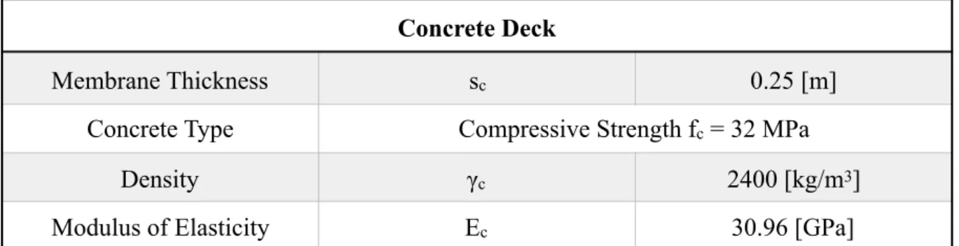
3.1.3. Concrete Deck

A concrete deck will be considered in order to emulate part of the self-weight of the structure. The main characteristics are reported in table 3.1-3 below:

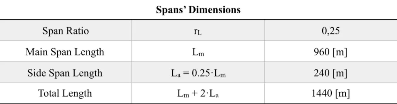
3.2. Defining Span Proportions and Lengths

First of all the total length of the suspension bridge has to be determined. The total length will be given by the length of the main span (Lm) and the two side-spans (2·La).

As far as the main span is regarded, a length of 960[m] is chosen for the ongoing analysis, a value that fits with practical experience. For the determination of the side spans’ length, reference can be made to “Cables Supported Bridges” (Gimsing 1997). Three-span suspension bridges are generally classified as:

• Suspension bridges with short side spans

!

• Suspension bridges with long side spans

!

An initial length ratio of 0.25 is therefore chosen, thus leading to the dimensions reported in Table 3.2 below:

Table 3.1-2

Cables and Hangers’ Properties

Modulus of Elasticity E 200 [GPa]

Design Stress fcbd 800 [MPa]

Density γcb 7850 [kg/m3_]

Table 3.1-3 Concrete Deck

Membrane Thickness sc 0.25 [m]

Concrete Type Compressive Strength fc = 32 MPa

Density γc 2400 [kg/m3_]

Modulus of Elasticity Ec 30.96 [GPa]

L_a≤ 0.3⋅ L_m

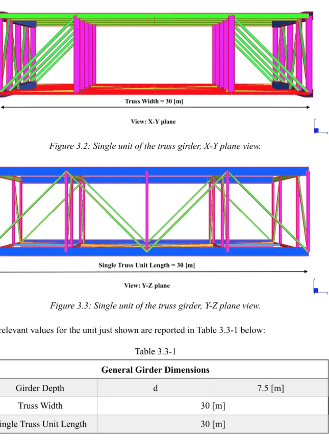
3.3. Truss Girder

The truss girder model is based on the Golden Gate Bridge’s girder, designed with the help of the available images and a similar model kindly provided by Professor Peter Ansourian of The University of Sydney. As the main focus of this work is to compare theoretical and software-based results, the elements composing the truss girder were not designed in detail but in order to obtain a reasonable model to be adopted in further analysis. A series of images are shown below depicting the structure of a single unit of the truss girder (Figures 3.1 - 3.2 - 3.3). This unit is thirty (30) meters wide , thirty (30) meters long and seven and a half (7.5) meters in depth. This unit will be copied along the z-axis in order to form the 1440 [m] long girder:

!

Figure 3.1: Single unit of the truss girder. Table 3.2

Spans’ Dimensions

Span Ratio rL 0,25

Main Span Length Lm 960 [m]

Side Span Length La = 0.25·Lm 240 [m]

!

Figure 3.2: Single unit of the truss girder, X-Y plane view.

!

Figure 3.3: Single unit of the truss girder, Y-Z plane view.

The relevant values for the unit just shown are reported in Table 3.3-1 below:

The following chart (Table 3.3-2) contains a list and relevant details of the elements adopted for the truss girder model. The Strand7 notation for structural elements’ dimensions is also reported in the right bottom side of the chart:

Table 3.3-1

General Girder Dimensions

Girder Depth d 7.5 [m]

Truss Width 30 [m]

The Uniformly Distributed Load (UDL) due to the girder and concrete deck’s self weight to be adopted in future calculations are reported in Table 3.3-3 below:

Table 3.3-2

Truss Girder’s Elements

Beam Property 1

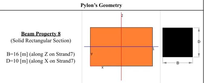
(Square Hollow Section) B=D=0.8 [m] T1=T2=0.02 [m] — A=0.0624 [m2_] I11=0.00633152 [m4] Beam Property 2 (RHS 250x150x9) B=0.15 [m] D=0.25 [m] T1=T2=0.009 [m] Beam Property 3 (IPE 500) B1=B2=0.20 [m] D=0.50 [m] T1=T2=0.016 [m] T3=0.0102 [m] Beam Property 4 (RHS 250x150x9) B=0.15 [m] D=0.25 [m] T1=T2=0.009 [m] Beam Property 5 (RHS 250x150x9) B=0.15 [m] D=0.25 [m] T1=T2=0.009 [m] A=0.0066 [m2_] I11=0.00005370 [m4] Beam Property 6 (IPE 600) B1=B2=0.22 [m] D=0.60 [m] T1=T2=0.019 [m] T3=0.012 [m] Beam Property 7 (RHS 250x150x9) B=0.15 [m] D=0.25 [m] T1=T2=0.009 [m] ! ! ! Table 3.3-3

Dead Load Determination - Self Weight Only

Continuous Structural Elements Over the Entire Length of the Bridge

Element Name UDL [kN/m] % of Total Load

Beam Property 1 19,22 1,36

Beam Property 4 1,44 0,10

Beam Property 5 1,02 0,07

Note: in the calculation listed in the following paragraphs, half of the UDL has to be considered because there are two planes of cables supporting the bridge. Reference will thus be made to (gtot/2):

!

3.4. Hangers

A. Central Hanger’s Length

The central hanger’s length is usually in the range of 3-10[m] (Gimsing 1997). For the purpose of the ongoing investigation a value of 3[m] has been selected.

Once the main cable’s sag will be known, the top pylon’s coordinate will be given by the summation of the central hanger’s length and the sag itself. All the other hangers will be ultimately connected once the cables and the truss girder are modelled. The design value is reported in Table 3.4-1:

Non Continuous Structural Elements

Element Name UDL [kN/m] % of Total Load

Beam Property 2 208 14,72

Beam Property 3 367 25,91

Beam Property 6 493 34,84

Beam Property 7 147 10,41

Concrete Deck

Element Name UDL [kN/m] % of Total Load

Plate Property 1 176,58 12,48

Resulting Total Dead Load (g) gtot = 1415 kN/m

g_tot

2 = 707.5 kN/m

Table 3.4-1

Central Hangers’ Length

B. Hangers’ Spacing

In order to properly model the connection between the girder and the suspension cables, the hanger spacing (λ) needs to be predetermined. Once again a value of 15[m] (reported in Table 3.4-2) is chosen following practical examples (the Golden Gate Bridge has the same spacing).

C. Hangers’ Diameter

The hangers’ diameter is determined by following the preliminary design guidelines given in “Cables Supported Bridges” (Gimsing 1997). There are two assumption on which this calculation is based:

i. The hangers will carry the distributed load acting on a length of the stiffening girder equal to the hanger spacing (λ).

ii. Concentrated forces (P) are represented by a uniformly distributed load acting on a length equal to thirty times the depth of the girder (30·d).

Given these assumptions and the relative scheme shown in Figure 3.4 below, the maximum hanger force is determined as:

!

!

Figure 3.4: Loading case for maximum hanger force (Gimsing 1997). Table 3.4-2

Hangers’ Spacing

λ 15 [m]

T_h= g + p

(

)

Considering that:

!

Note that the traffic and concentrated loads are neglected at this stage because their contribution is negligible compared to that of self weight. Moreover, concentrated forces are assumed to be redistributed along a length equal to thirty times the depth of the girder:

!

The cross-sectional area can now be determined as:

!

Hence the diameter for all the hangers will be (as reported in Table 3.4-3):

!

As shown in Figure 3.5 below, the hangers will be connected to the girder with a spacing of λ=15 [m]:

!

Figure 3.5: Hangers’ connection to the truss girder. g= gtot 2 = 707.5 kN/m p= 0 kN/m P= 0 kN d= 7.5 m λ = 15 m ⎧ ⎨ ⎪ ⎪ ⎪ ⎪ ⎩ ⎪ ⎪ ⎪ ⎪ ⇒ T_h= 10612 kN P λ 30⋅ d = P 15 30⋅7.5= 1 15P A_h= Th f_cbd = 10612⋅103 800 = 0.013 m 2 D_h= 4⋅ Ah π ! 0.130 m Table 3.4-3 Hangers’ Diameter Dh 0.150 [m]

3.5. Cables’ Profile Definition and Preliminary Design

In order to model the suspension cables on Strand7 it is necessary to first determine the shape to be adopted (catenary or parabola). Strand7 permits the user to model a “cable” element but this would not be composed of the nodes required to connect the suspension cables to the stiffening girder by means hangers. It is therefore required to create the nodes of the suspension cable as points of a parabolic or catenary curve. An investigation of the accuracy of the two shapes is carried out in the following paragraph.

3.5.1. Catenary VS Parabola

In order to decide if the shape to be adopted is the one of the catenary or the parabola, a brief example will be shown below. As already discussed in the literature review, the catenary curve and the parabolic curve diverge at a sag ratio of 0.15 (Walter Podolny 1976). In order to verify the accuracy of this result, two cables having different sag ratios have been modelled using both the catenary and the parabolic equations. The design parameters and relevant dimensions are reported in Table 3.5-1 below.

• Step 1 - Modelling the cable on Strand7

The horizontal component of tension in the cable T0 is due to the cable’s self weight only. The two cables just analysed have no internal nodes to be connected to hangers. The following step is therefore necessary to create these nodes.

• Step 2 - Creating the Catenary and Parabolic Curved Cable

Once the horizontal component of the tension (T0) in the cable is known, its value can be used and substituted in the equation for the catenary provided in paragraph 2.1.1. The sag value

Table 3.5-1

Relevant Design Parameters Cable_1 Cable_2

Diameter (D) 0.934 [m] 0.934 [m]

Horizontal Chord’s Length (L) 1260 [m] 1260 [m]

Cable’s Free Length (l) 1550 [m] 1307 [m]

Sag (d) 399,0987 152.0939 [m]

Sag Ratio (d/L) 0,32 0,12

Horizontal Component of Tension (T0) 29,188,471.69 [N] 70,099,084.39 [N] 52,762.08 [N/m] 52,762.08 [N/m] Weight of cable/unit length (! )µ

obtained from the catenary equation is then used in the determination of the parabolic shape of the cable (following the formulas in paragraph 2.1.2). This way, given the same sag “d” for the two shapes, an evaluation of the most accurate shape can be carried out:

!

!

The sag value “dc”, obtained from the catenary equation, and the horizontal component of tension in the cable “H” for the two analysed cables are reported in Table 3.5-2 below:

The obtained sets of coordinates are reported in Tables A3.1 and A3.2 in the Appendix and can be copied and pasted on Strand7 in order to create the connection nodes for the sagging cables. These nodes will then be connected with “cutoff bar” elements in order to model the suspension cables for the bridge’s model.

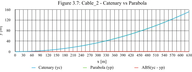
• Step 3 - Verifying the Accuracy of Results

The obtained profiles are plotted in Figures 3.6 and 3.7 below:

! Catenary: y= c⋅cosh x c ⎛ ⎝⎜ ⎞ ⎠⎟ = T₀ µ ⋅ cosh xµ T₀ ⎛ ⎝⎜ ⎞ ⎠⎟−1 ⎡ ⎣ ⎢ ⎢ ⎤ ⎦ ⎥ ⎥ Parabola: y=1 2 µ H⋅ x 2 H= µL2 8d_c ⎧ ⎨ ⎪ ⎪ ⎩ ⎪ ⎪ Table 3.5-2

Obtained Results Cable_1 Cable_2

dc 399.2092 [m] 152.1890 [m]

H 26,228,442.28 [N] 68,800,17.06 [N]

Figure 3.6: Cable_1 - Catenary vs Parabola

y [m ] 0 100 200 300 400 x [m] 0 30 60 90 120 150 180 210 240 270 300 330 360 390 420 450 480 510 540 570 600 630

!

As it can be noticed from the plots shown above the discrepancy between the catenary and the parabolic curve for Cable_1 (having sag ratio equal to 0.32) is greater than the one for Cable_2 (having a sag ratio of 0.12). This agrees with our expectation as the sag ratio for Cable_1 is larger than 0.15. In particular, the maximum discrepancy on the y-axis for the two cables are reported in Table 3.5-3 below:

Moreover, there is a small discrepancy between the sag given by Strand7 and the catenary equation. This is probably due to the accuracy of the horizontal component of tension in the cable obtained on Strand7 and to be used as an input for the catenary equation. However, this does not represent a problem as the 0.03% - 0.06% error observed does not affect any design factor. These discrepancies are reported in Table 3.5-4 below:

Conclusions:

The parabolic curve represents the shape adopted by the freely hanging cable with a satisfying accuracy for sag ratios smaller than 0.15. For this reason, both the catenary and the parabolic shapes can be adopted for the model of the suspension bridge as its sag ratios are usually in

Figure 3.7: Cable_2 - Catenary vs Parabola

y [m ] 0 40 80 120 160 x [m] 0 30 60 90 120 150 180 210 240 270 300 330 360 390 420 450 480 510 540 570 600 630

Catenary (yc) Parabola (yp) ABS(yc - yp)

Table 3.5-3

Maximum discrepancy Cable_1 Cable_2

max (yc - yp) 10.34 [m] 0.71 [m]

max (yc - yp)/d 2,6% 0,46%

Table 3.5-4

d (Strand7) dC (Catenary Eq.) Discrepancy

Cable_1 399,0987 399,2092 0,03%

the range 0.08 - 0.12. It is therefore plausible to rely on the simplified equations based on the parabolic shape that can be often encountered in literature.

The procedure adopted for the creation of the nodes on Strand7 will not be shown again in the ongoing analysis as it is the same as the one just presented.

3.5.2. Main Suspension Cable

A. Sag Ratio and Cable Profile Definition

The first parameter to be determined at this stage is the sag ratio of the main cable. As already reported in the literature review, typical sag ratios for the main span are in the range of 0.08-0.12 (Pugsley 1968; Gimsing 1997). The chosen value for the purpose of this project and the resultant sag are therefore reported in Table 3.5-5 below:

The chosen sag ratio represents a good compromise for material and stiffness optimisation: a larger sag would minimise the use of material whilst a smaller sag would improve stiffness (Gimsing 1997).

The adopted value of the diameter is initially assumed as 0.8[m] (as reported in Table 3.5-6), similarly to the one adopted for the Golden Gate Bridge’s suspension cable.

This initial diameter will be probably refined in the following paragraphs and its value may actually change. However, having a pre-defined geometry eases the initial Strand7 phases of modelling in which it might be interesting to test the single cable itself. In fact, when testing the cable alone, the girder’s properties and thus its dead load might not be known.

It can be now modelled the single “cable” element on Strand7 in order to get the value of the horizontal component of tension in the cable (T0) due to self-weight, to be adopted for the

Table 3.5-5

Sag and Sag Ratio - Preliminary Assumption

k*m 96 [m]

s*r,m 0,10

Table 3.5-6

Diameter - Preliminary Assumption

Diameter D1 0.8 [m]

determination of the catenary’s nodes. The procedure has already been explained in the previous paragraph and will not be entirely reported here.

Strand7 will require to insert a “cable free length” value that matches with the designed sag. Instead of guessing this value, reference can be made to formula (10) of paragraph 2.1.2 of the Literature Review in order to have an accurate estimation. In this situation we can notice how parabola-based formulas can be useful. The formula is rewritten here using the Gimsing notation:

!

The resulting sag given in Strand7 will be slightly different from the one initially assumed (96 m) as reported in Table 3.5-7 below:

However, this discrepancy does not represent an issue as the sag ratio has changed by 2% only. The obtained sag value is to be used in all the following calculations.

The horizontal component of the tension in the cable obtained via Strand7 analysis is reported in Table 3.5-8:

Once again it is interesting to compare the Strand7’s result for T0 with the one given in paragraph 2.1.2. (rewritten for Gimsing notation). The horizontal component of tension in the cable given by the parabola-based formula is:

! L_{m, f} = L_m⋅ 1+8 3 k_m* L_m ⎛ ⎝ ⎜ ⎜ ⎞ ⎠ ⎟ ⎟ 2 ⎡ ⎣ ⎢ ⎢ ⎢ ⎤ ⎦ ⎥ ⎥ ⎥ = 985.60 m Table 3.5-7

Design Sag and Sag ratio - Strand7 Model

km 97.83 [m]

sr,m 0,102

Table 3.5-8

Horizontal Component of Tension in the Cable

T0 46200.41 [kN]

T_{0, parabolic shape}= µm⋅ L2m

The 1.4% discrepancy is acceptable and once again underlines how useful the simplified parabolic-based analysis can be.

It is now possible to evaluate the pylon top coordinate (reported in Table 3.5-9 below). As the (y)-reference plane is located at the top layer of the truss girder (it coincides with the top elements’ axis), this will be situated at:

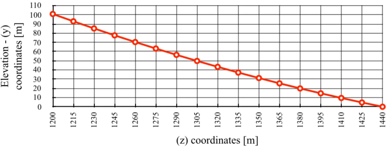
This coordinate is also used to evaluate the side span cable shape in the relevant paragraph. By substituting the proper values in the catenary equation already presented we get the nodes of the sagging cable. The step (∆z) to be adopted has to be equal to the hanger spacing (λ) in order to connect the truss girder to the suspension cable with vertical elements (hangers):

!

The plot showing the nodes and the cable shape (the right half of it) is schematically shown in Figure 3.8 below (not in scale):

!

Figure 3.8: Catenary shape for the Strand7 model.

The obtained coordinates are also reported in Table A3.3 in the Appendix.

Note that the bottom left node represented in the plot corresponds to the cable’s node at midspan, having the following coordinates:

Table 3.5-9

Pylon Top (y) coordinate

Hpt km + jm 100.83 [m] y= T0 µ_m⋅ cosh zµ_m T₀ ⎛ ⎝⎜ ⎞ ⎠⎟−1 ⎡ ⎣ ⎢ ⎢ ⎤ ⎦ ⎥ ⎥ E le va ti on - (y) coordi na te s [m ] 0 10 20 30 40 50 60 70 80 90 100 110 (z) coordinates [m] 720 735 750 765 780 795 810 825 840 855 870 885 900 915 930 945 960 975 990 _{1005 1020 1035 1050 1065 1080 1095 11}10 _{1125 1140 1155 1170 1185 1200}

!

Whilst the top right node corresponds to the cable’s node at the top of the pylon, having the following coordinates:

!

The so obtained cable will be mirrored on Strand7 in order to obtain the entire main cable.

B. Refining the Main Cable’s Diameter

Now that the main elements composing the model are defined, it is possible to refine the diameter of the main cable, reference is made to the book “Cable Supported Bridges” (Gimsing 1997). If the following assumptions are adopted:

i. The hangers’ dead load can be neglected as its contribution is quite small

ii. Traffic load (p) and concentrated forces (P) are neglected at this stage because they are usually negligible compared to the girder’s self weight

Then the area of the cable can be calculated as:

!

Where:

!

Hence the diameter:

!

The adopted refined value is thus reported in Table 3.5-10: y , z

( )

(

)

( )

(

)

(

)