Forecast of high-impact weather over Italy: performance of global and limited-area ensemble prediction systems

(1)

Alma Mater Studiorum

_{· Universit`a di Bologna}

Scuola di Scienze

Corso di Laurea Magistrale in Fisica del Sistema Terra

Forecast of High-Impact Weather over

Italy: performance of global and

limited-area ensemble prediction systems

Relatore:

Prof.ssa Silvana Di Sabatino

Correlatori:

Dott. Andrea Montani

Dott.ssa Tiziana Paccagnella

Presentata da:

Giacomo Pincini

Sessione I

(2)

(3)

Sub lumine Matris

(4)

(5)

Sommario

Nella previsione del tempo l’approccio deterministico non permette di sta-bilire a priori se una previsione sará corretta o meno; d’altra parte, le previ-sioni probabilistiche forniscono un punto di vista piú completo, affidabile e accurato di che cosa potrebbe accadere nel futuro, dando idealmente infor-mazioni sulla relativa frequenza dell’evento. Quindi apportano precisi van-taggi per coloro che devono prendere delle decisioni. Gli utenti delle pre-visioni possono sfruttare queste informazioni per esempio quando vogliono valutare le perdite associate a condizioni meteo avverse, rispetto ai costi delle azioni preventive. Lo scopo di questo lavoro é valutare il valore ag-giunto di una migliore risoluzione orizzontale nella previsione probabilistica dei campi in quota e alla superficie. In particolare, sono state confrontate le performance di tre differenti sistemi di previsione di ensemble: ECMWF-ENS (51 membri, risoluzione orizzontale 18km), COSMO-LEPS (16 mem-bri, risoluzione orizzontale 7km) e COSMO-2I-EPS (10 memmem-bri, risoluzione orizzontale 2.2km). Mentre i primi due sistemi di ensemble sono operativi, COSMO-2I-EPS é ancora in fase di sviluppo. Pertanto, la finestra di com-parazione copre un periodo limitato: dal 20 al 27 giugno 2016. In questo lavoro, sono state analizzate sia le variabili in quota che al suolo. Le vari-abili in quota, considerate a tre differenti livelli di pressione, sono l’altezza di geopotenziale e la temperatura; per la verifica sono stati calcolati l’ensemble spread e la radice dell’errore quadratico medio, utilizzando i dati dei ra-diosondaggi italiani disponibili ogni 12/24 ore. Le variabili al suolo, tem-peratura a 2 metri e precipitazione cumulata su 6 ore, sono state verificate tramite la rete di stazioni non convenzionali fornite dal Dipartimento di Pro-tezione Civile Nazionale. Per la temperatura a 2 metri sono stati calcolati

(6)

l’ensemble spread e la radice dell’errore quadratico medio, mentre per la pre-cipitazione sono stati considerati alcuni score probabilistici (Brier Skill Score, Ranked Probability Score, ROC-Area, Percentuale di Outliers ed altri). Sia per la verifica in quota che per quella alla superficie, gli score migliori sono stati ottenuti principalmente dai sistemi di ensemble del consorzio COSMO. Questi si caratterizzano per avere una risoluzione orizzontale piú alta e una popolazione di membri piú bassa. In particolare, il recentemente implemen-tato COSMO-2I-EPS raggiunge spesso le performance piú soddisfacenti. A causa della limitata disponibilitá di dati, i risultati di questo studio pilota si basano su un periodo relativamente breve, pertanto sono necessarie ul-teriori analisi. Ciononostante, nei sistemi di ensemble alla mesoscala, il valore aggiunto dell’alta risoluzione sembra giocare un ruolo cruciale nella previsione probabilistica dei campi atmosferici a tutti i livelli. In partico-lare, negli ensemble di COSMO, la descrizione piú dettagliata dei processi connessi all’orografia fornisce un valore aggiunto per la previsione di eventi meteorologici localizzati ad elevato impatto.

(7)

(8)

Abstract

The deterministic approach to weather prediction does not allow to estab-lish a-priori whether a forecast would be skilful or unskillful; on the other hand, probabilistic forecasts provide a more complete, reliable and accurate view of what could happen in the future, ideally providing information on the relative frequency of the event. Therefore, they bring definite benefits for decision-makers. Forecast users can exploit such information for exam-ple when they want to weight the losses associated with adverse weather events against the costs of taking precautionary actions. The aim of this work is to assess the added value of the enhanced horizontal resolution in the probabilistic prediction of upper-level and surface fields. In particular, the performances of three different ensemble prediction systems were compared: ECMWF-ENS (51 members, 18 km horizontal resolution), COSMO-LEPS (16 members, 7 km horizontal resolution) and COSMO-2I-EPS (10 mem-bers, 2.2 km horizontal resolution). While the first 2 ensemble systems are operational, COSMO-2I-EPS is still in a development phase. Therefore, the intercomparison window covers a limited period, which ranges from 20 to 27 June 2016. In this work, both upper-level and surface variables are analyzed. As for upper-level, both temperature and the geopotential height at three different pressure levels are considered; the ensemble spread and the root mean square error are computed using the available Italian radiosounding data every 12/24 hours for verification. As for the surface, 2-metre tem-perature and precipitation cumulated over six hours are verified against the non-conventional station network provided by the National Civil Protection Department. The ensemble spread and the root mean square error of 2-metre temperature are computed, while a number of probabilistic scores (Brier Skill

(9)

Score, Ranked Probability Score, Roc-Area, Outliers Percentage and others) are considered for precipitation.

For both upper-level and surface verification, it turns out that the best scores are mainly obtained by the COSMO-based ensemble systems with higher horizontal resolution and lower ensemble size; in particular, the newly implemented COSMO-2I-EPS often achieves the most satisfactory perfor-mances.

Although the results of this pilot study are based over a relative short pe-riod due to limited data availability and further investigations is needed, the added value of high resolution in mesoscale ensemble systems seems to play a crucial role in the probabilistic prediction of atmospheric fields at all levels. In particular, the more detailed description of mesoscale and orographic-related processes in COSMO-ensembles provides an added value for the prediction of localised High-Impact Weather events.

(10)

(11)

List of Figures

1.1 Maps of total precipitation cumulated over 24 hours for the 27th June 2016: on the top observations from rain gauges of DPCN, in the bottom left as was predicted by the run of 26th June 00 UTC from member 1 of ECMWF ENS, on the bottom right the same but for COSMO-LEPS. . . 3 2.1 Grid points over Europe of ECMWF model (souce: ECMWF). 7 2.2 Vertical levels of the ECMWF model in previous versions

(source: ECMWF). . . 8 2.3 Type of observations used to estimate the atmosphere initial

conditions in a typical day (source: ECMWF). . . 9 2.4 Map of radiosonde locations (source: ECMWF). . . 9 2.5 Schematic diagram of the different physical processes

repre-sented in the ECMWF model (source: ECMWF). . . 10 2.6 The predictability problem may be explained in terms of the

time evolution of an appropriate probability density function (PDF). Ensemble prediction based on finite number of deter-ministic integration seems to be a feasible method to predict the PDF beyond the range of linear growth (source: ECMWF). 12

(14)

2.7 Schematic of a probabilistic weather forecast using initial con-dition uncertainties. The blu lines show the trajectories of the individual forecasts that diverge from each other owing to un-certainties in the initial conditions and in the representation of sub-grib scale processes in the model. The main goal is to explore all the possible future states of the atmosphere. The dashed, lighter blue envelope represents the range of possible states that the real atmosphere could encompass and the solid, dark blue envelope represents the range of states sampled by the model predictions. A good forecast is the one which anal-ysis lies inside the ensemble spread (source: ECMWF). . . 14 2.8 Lorenz attractor with superimposed finite-time ensemble

inte-gration (source: ECMWF). . . 16 2.9 ECMWF forecasts for air temperature in London started from

(a) 26 June 1995 and (b) 26 June 1994 (source: ECMWF). . . 18 3.1 The ECMWF total convective rainfall forecast from 28

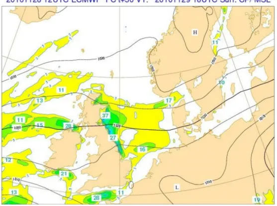
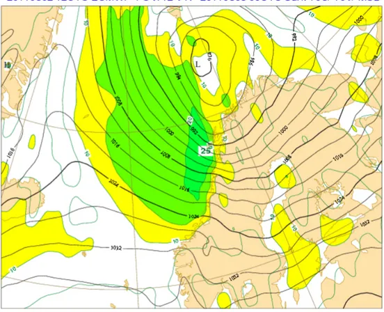
Novem-ber 2010 12 UTC +30h. The convection scheme has difficulty in advecting wintery showers inland over Scotland and north-ern England from the relatively warm North Sea. The con-vection scheme is diagnostic and works on a model column, so cannot produce large amounts of precipitation over the rela-tively dry and cold (stable) wintery land areas. In nature these showers succeed in penetrating inland through a convectively induced upper-level warm anomaly leading to large-scale lift-ing and saturation (source: ECMWF). . . 26 3.2 MSLP and 10 m wind forecast from 2 March 2011 12 UTC

+12h. The 10 m winds are unrealistically weak over the rugged Norwegian mountains. Value of 10 m/s might be realistic in sheltered valleys, but not on exposed mountain ranges (source: ECMWF). . . 27

(15)

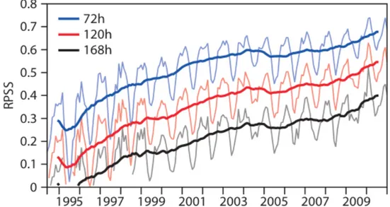
3.3 A skill measure for forecasts of the 850 hPa temperature over the northern hemisphere (20o-90oN) at days 3, 5 and 7. Com-paring the skill measure at the three lead times demonstrates that on average the performance has improved by two days per decade. The level of skill reached by a 3-day forecast around 1998/99 (skill measure = 0.5) is reached in 2008/09 by a 5-day forecast. In other words, today a 5-day forecast is as good as a 3-day forecast 10 years ago. The skill measure used here is the Ranked Probability Skill Score (RPSS), which is 1 for a perfect forecast and 0 for a forecast no better than climatology (from ECMWF User Guide). . . 29

3.4 A grid box volume ∆V = ∆ζ∆λ∆φ showing the

Arakawa-C/Lorenz (Arakawa et al. 1977) staggering of the dependent model variables. ζ, λ and φ refer to the coordinate system. . . 32 3.5 COSMO-2I-EPS integration domain. . . 37 3.6 Representation of the orography (in metre) over part of

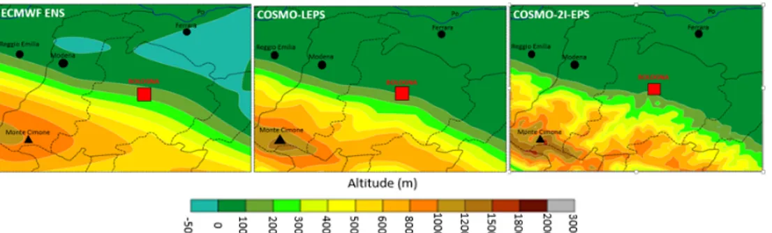
Emilia-Romagna according to ECMWF ENS (left panel), COSMO-LEPS (middle panel) and COSMO-2I-EPS (right panel). . . . 38

4.1 Reanalysis from ERA-Interim (ECMWF) valid at 00 UTC

of 20th June: colours discriminate different value of 500 hPa height (in dam); solid white line link point with same MSLP (interpolated by Meteociel (www.meteociel.fr)). . . 41 4.2 Reanalysis from ERA-Interim (ECMWF) valid at 00 UTC of

20th_{June: colours discriminate different velocity of jet stream}

at 300 hPa height (in km/h), arrows show wind direction. . . . 42 4.3 Reanalysis from ERA-Interim (ECMWF) valid at 00 UTC of

20th _{June: colours discriminate different air temperature at}

850 hPa height (in o_{C). . . .} ₄₃

4.4 Synoptic chart valid at 00 UTC of 20th June 2016, by UK Met Office. . . 44

(16)

4.5 Satellite image of 20th June 2016 00 UTC from EUMETSAT (European Meteorological Satellites) in the infrared channel (MET10 RGB-Airmass). . . 45 4.6 (a) Reanalysis from ERA-Interim (ECMWF) valid at 00 UTC

of 23th _{June: colours discriminate different value of 500 hPa}

height (in dam); solid white line link point with same MSLP (interpolated by Meteociel (www.meteociel.fr)). (b) Synoptic charts valid at 00 UTC of 23th _{June 2016, by UK Met Office.}

(c) Satellite image of 23th _{June 2016 00 UTC from}

EUMET-SAT in the infrared channel (MET10 RGB-Airmas). . . 46 4.7 (a) Reanalysis from ERA-Interim (ECMWF) valid at 00 UTC

of 26th June: colours discriminate different value of 500 hPa height (in dam); solid white line link point with same MSLP (interpolated by Meteociel (www.meteociel.fr)). (b) Synoptic charts valid at 00 UTC of 26th _{June 2016, by UK Met Office.}

(c) Satellite image of 26th _{June 2016 18 UTC from}

EUMET-SAT in the infrared channel (MET10 RGB-Airmas). . . 47 4.8 (a) Reanalysis from ERA-Interim (ECMWF) valid at 00 UTC

of 27th June: colours discriminate different value of 500 hPa height (in dam); solid white line link point with same MSLP (interpolated by Meteociel (www.meteociel.fr)). (b) Synoptic charts valid at 00 UTC of 27th June 2016, by UK Met Of-fice. (c) Satellite image of 27th _{June 2016 00 UTC from}

EU-METSAT in the infrared channel (MET10 RGB-Airmas). (d) Satellite image of 27th _{June 2016 18 UTC from EUMETSAT}

in the infrared channel (MET10 RGB-Airmas). . . 48 4.9 Total precipitation (mm) collected from rain gauges of DPCN

(Dipartimento di Protezione Civile Nazionale) network, from 20th June 2016 at 00 UTC to 29th June 2016 at 00 UTC. The lack of some stations (e.g in Trentino Alto Adige) is due to the partial unavailability of data during the investigation period. . 50

(17)

4.10 The interpolation uses the four corner points closest to the selected location and takes a weighted average to arrive at the interpolated value where u and v are non-dimensional weight-ing factors that vary between 0 and 1 across the blue grid (from ECMWF Forecast User Guide). . . 51 5.1 The domain, centered over Italy, considered for the verification

of the three ensemble systems. . . 61 5.2 The position of radiosoundings within the domain. . . 63 5.3 The position of the stations of the Northern-Italy non-GTS

network within the domain. . . 64 5.4 The position of DPCN stations within the domain. . . 65 5.5 (a) The position of DPCN stations within the domain; (b)

the position of DPCN plain stations within the domain; (c) the position of DPCN hill stations within the domain; (d) the position of DPCN mountain stations within the domain. . . . 66 5.6 The figure shows the spreads (continuous lines) and the RMSE

(dotted lines) values for three pressure levels indicated in the captions. The results are obtained for the 48 hours of the fore-cast range every 12 hours. The ECMWF EPS scores appear in red, COSMO-LEPS in blue and COSMO-2I-EPS in green. The forecast range (in hours) is shown in the abscissa whereas in the ordinate the value of spread and RMSE (in m) is shown. All details are indicated in the legend at the top left of each figure. . . 68 5.7 The table shows the spread and RMSE values for the

geopo-tential height averaged over the entire forecast range. The results are sorted by ensemble system (in rows) and by pres-sure levels, hence spreads and RMSE (in columns). For each class of values (spread or RMSE), it is pointed out in bold which of the three values (one for every ensemble) is the best. 69

(18)

5.8 The figure shows the spreads (continuous lines) and the RMSE (dotted lines) values for three pressure levels indicated in the captions. The results are obtained for the 48 hours of the forecast range every 12 hours. The ECMWF EPS scores ap-pear in red, COSMO-LEPS in blue and COSMO-2I-EPS in green. The forecast range (in hours) is shown in the abscissa whereas in the ordinate the value of spread and RMSE (ino_C)

is shown. All details are indicated in the legend at the top left of each figure. . . 71 5.9 The table shows the spread and RMSE values for the

temper-ature averaged over the entire forecast range. The results are sorted by ensemble system (in rows) and by pressure levels, hence spreads and RMSE (in columns). For each class of val-ues (spread or RMSE), it is pointed out in bold which of the three values (one for every ensemble) is the best. . . 72 5.10 The figure shows the spreads (continuous lines) and the RMSE

(dotted lines) values obtained for the 48 hours of the forecast range every 6 hours. The ECMWF EPS scores appear in red, COSMO-LEPS in blue and COSMO-2I-EPS in green. The foreacst range (in hours) is shown in the abscissa, in the or-dinate the value of spread and RMSE (in oC). All details are indicated in the legend at the top left. . . 74 5.11 The figure shows the BSS for the three ensemble systems

(ECMWF ENS in red, COSMO-LEPS in blue, COSMO-2I-EPS in green) and for the threshold of 1 mm (continuous line) and 10 mm (dotted line). The forecast range of 48 hours, in 6-hour steps, is shown in the abscissa. The dimensionless val-ues of the BSS are marked in ordinate. In particular, a black line was placed for BSS=0. Negative values of BSS indicate a forecast skill lower than climatology. . . 76

(19)

5.12 The figure shows the RPS for the three ensemble systems (ECMWF ENS in red, COSMO-LEPS in blue, COSMO-2I-EPS in green). The forecast range of 48 hours, in 6-hour steps, is shown in the abscissa; the dimensionless values of the RPS are marked in the ordinate. . . 78 5.13 The figure shows the RPS for four different observational dataset,

indicated in the caption under each image. The ensemble systems are ECMWF ENS in red, COSMO-LEPS in blue, COSMO-2I-EPS in green. The forecast range of 48 hours, in 6-hour steps, is shown in the abscissa; the dimensionless values of the RPS are marked in the ordinate. . . 79 5.14 The figure shows the RP SSD for the three ensemble systems

(ECMWF ENS in red, COSMO-LEPS in blue, COSMO-2I-EPS in green). The forecast range of 48 hours, in 6-hour steps, is shown in the abscissa. The dimensionless values of the BSS are marked in the ordinate. In particular, a black line was placed for RP SSD = 0. Negative values of RP SSD

indicate a forecast skill lower than climatology. . . 81 5.15 The figure shows the RP SSD for four different observational

dataset, indicated in the caption under each image. The en-semble systems are ECMWF ENS in red, COSMO-LEPS in blue, COSMO-2I-EPS in green. The forecast range of 48 hours, in 6-hour steps, is shown in the abscissa; the dimen-sionless values of the RP SSD are marked in the ordinate. In

particular, a black line was placed for RP SSD = 0. Negative

values of RP SSD indicate a forecast skill lower than climatology. 83

5.16 The figure shows the ROC Area for the three ensemble systems (ECMWF ENS in red, COSMO-LEPS in blue, COSMO-2I-EPS in green) and for the threshold of 1 mm (continuous line) and 10 mm (dotted line). The forecast range of 48 hours, in 6-hour steps, is shown in the abscissa. The dimensionless values of the ROC Area are marked in the ordinate. . . 84

(20)

5.17 The figure shows the percentage of outliers for the three en-semble systems (ECMWF ENS in red, COSMO-LEPS in blue, COSMO-2I-EPS in green). The forecast range of 48 hours, in 6-hour steps, is shown in the abscissa. The percentage of out-liers is marked in the ordinate. . . 85 5.18 The figure shows the percentage of outliers for four different

observational dataset, indicated in the caption under each im-age. The ensemble systems are ECMWF ENS in red, COSMO-LEPS in blue, COSMO-2I-EPS in green. The forecast range of 48 hours, in 6-hour steps, is shown in the abscissa; the per-centage of outliers is marked in the ordinate. . . 87 5.19 In the table for each step of the forecast range, the values

for RP S, RP SSD and percentage of outliers, for both

verifi-cation methods(nearest grid point and bilinear interpolation) are written. In order to help the reader in the comparison, the digits that change from one method to another have been underlined. . . 88 5.20 Boxplots for the total precipitation cumulated over 24-hours

on 27th June 2016: in yellow the observations from the rain gauges of the DPCN, in red as expected by the member 1 of ECMWF ENS with the forecast range +24-48h, in blu and in green the same but for COSMO-LEPS and COSMO-2I-EPS respectively. . . 90 5.21 Boxplots for the total precipitation cumulated over 6-hours

on 27th _{June 2016: in yellow the observations from the rain}

gauges of the DPCN, in red as expected by the member 1 of ECMWF ENS with the forecast range +24-48h, in blu and in green the same but for COSMO-LEPS and COSMO-2I-EPS respectively. Time slots are indicated in the titles of the figures. 92

(21)

5.22 Boxplots for the total precipitation cumulated over 24-hours on 27th June 2016: in yellow the observations from the rain gauges of the DPCN, in red as expected by the member 1 of ECMWF ENS with the forecast range +24-48h, in blu and in green the same but for COSMO-LEPS and COSMO-2I-EPS respectively. The intensity categories are indicated in the titles of the figures. . . 93 6.1 Maps of total precipitation cumulated over 24 hours for the

27th June 2016: at the top left observations from rain gauges of DPCN, at the top right as was foreseen by the run of 26th June 00 UTC from the member 1 of COSMO-2I-EPS, at the bottom left and bottom right the same but for ECMWF ENS and COSMO-LEPS respectively. . . 98

(22)

List of Tables

4.1 The contingency table . . . 57 5.1 geopotential height and temperature verification features . . . 65 5.2 2-metre temperature verification features . . . 73 5.3 6-hourly total precipitation verification features . . . 75

(23)

List of Acronyms

1. AISAM Associazione Italiana di Scienze dell’Atmosfera e del Clima 2. ARPA-SIMC Agenzia Regionale Prevenzione Ambientale - Servizio Idro

Meteo Clima 3. BS Brier Score 4. BSS Brier Skill Score

5. CAPE Convective Available Potential Energy 6. CFL Courant-Friedrichs-Lewy

7. COSMO COnsortium for Small-scale MOdeling 8. DPCN Dipartimento di Protezione Civile Nazionale 9. DWD Deutscher Wetterdienst

10. ECMWF European Centre for Medium-Range Weather Forecast 11. EDA Ensemble of Data Assimilation

12. EMS European Meteorological Society

13. ENIAC Electronic Numerical Integrator And Computer 14. ENS ENSemble

15. EPS Ensemble Prediction System 16. ERA European Reanalysis

(24)

17. EUMETSAT EUropean METeorological SATellites 18. GPS Global Positioning System

19. GTS Global Telecommunications Systems 20. HE-VI Horizontally Explicit, Vertically Implicit 21. HIW High-Impact Weather

22. HNMS Hellenic National Meteorological Service 23. HRES High-RESolution

24. H-TESSEL Hydrology-Tiled ECMWF Scheme for Surface Exchange over Land

25. ICs Initial Conditions

26. IFS Integrated Forecasting System 27. LAI Leaf Area Index

28. LEPS Limited area Ensemble Prediction System 29. LM Lokal Modell

30. ME Mean Error

31. MPI Message Passing Interface 32. MPP Massively Parallel Processing 33. MSE Mean Square Error

34. MSLP Mean Sea Level Pressure

35. NCEP National Centre for Environmental Prediction 36. NWP Numerical Weather Prediction

(25)

38. OUTL OUTLiers

39. PDF Probability Density Function 40. RASS Radio Acoustic Sounding System 41. RM Representative Member

42. RMSE Root Mean Square Error

43. ROC Relative Operating Characteristic Curve 44. RPS Ranked Probability Score

45. RPSS Ranked Probability Skill Score

46. RPSSD debiased Ranked Probability Skill Score

47. SPPT Stochastic Perturbations of Physical Tendencies 48. SPRD ensemble SPReaD

49. SST Sea Surface Temperature 50. SV Singular Vector

51. TVD Total Variation Diminishing 52. UTC Universal Time Coordinated 53. VAD Velocity Azimuth Display

(26)

Chapter 1 Introduction

The prediction of weather events related to strong winds, heavy rain and snowfall is still nowadays a serious challenge, especially when high spatio-temporal details are required. Despite Numerical Weather Prediction (NWP) modelling has made great progress in recent decades, thanks to the increases in model resolution, better understanding of atmospheric dynamical pro-cesses and advances in data assimilation techniques, the above-mentioned atmospheric events, usually referred to as “High-Impact Weather” (HIW), can have horizontal dimension too small to be explicitly resolved. HIWs pro-vide the most dramatic examples of how the atmosphere affects people daily lives, since they may cause both human and economic costs. Therefore, there is a need of better ways to predict this type of phenomena, also accounting for their inherent degree of non-predictability.

This paves the way to the introduction of a probabilistic approach via the ensemble forecasting, which was introduced at the beginning of the nineties, in order to provide a representation of model uncertainty, due to the imper-fect knowledge of atmospheric initial conditions and the approximate model formulation. This approach has now become commonplace in operational weather forecasting by the major meteorological institutes. Instead of run-ning just one forecast with an unknown error, an ensemble of slightly different forecasts are run, in order to integrate the deterministic forecast with an es-timate of the ”forecast of forecast skill” (Tennekes et al., 1986). Probabilistic forecasts provide a more complete, reliable and accurate view of what might

(27)

happen in the future, ideally providing information on the relative frequency of an event occuring. Therefore, they bring definite benefits for decision-makers. Forecast users can exploit such information for cost-loss analysis. The estimation of uncertainty is even more crucial when local effects come into play and a high spatio-temporal detail is required as in the case of pre-cipitation, where NWP limitations become more evident.

To understand the difficulty by medium–to–low horizontal resolution mod-els in forecasting this type of phenomena, it is presented the case of 27th _June

2016. On this day, two storm lines have crossed at different times some Ital-ian regions: those of the northeast during the first hours of the day, Umbria and Marches in the afternoon. In Fig. 1.1, it is possible to see both observed and forecast precipitation for the 27thJune 2016. The top left panel provides observed precipitation according to the rain gauges collected by the National Civil Protection Department (DPCN). On the other hand, the bottom left and right panels show 24-hour total precipitation as predicted by the model runs starting at 00 UTC of 26th _{June, respectively by the member 1 of global}

ensemble system ECMWF ENS and of the COSMO-based limited-area en-semble prediction system COSMO-LEPS.

Looking at the figure, it will be evident that both forecasts show some critical issues: there are marked inaccuracies both in the spatial localization and in the intensity of precipitation. In particular, the problems relate to the excessive extension of precipitation over northern Italy, the absence or inaccurate location of heavier rainfall and the lack or different pattern of precipitation that hit the central Italy. Thus there is room for improvement. This improvement can be sought using an ensemble system with a higher horizontal resolution. The new national ensemble system satisfies this re-quest. It is in a pre-operational phase, for this reason it is useful to study its performance against ensemble systems with a lower resolution.

Therefore the main purpose of this thesis is to assess the performance of the newly developed high-resolution ensemble prediction system for a number of HIW events similar to that reported in Fig. 1.1. It is planned to compare its performance against the above mentioned state-of-the-art ensemble pre-diction systems, both running on an operational basis. More precisely, the

(28)

Figure 1.1: Maps of total precipitation cumulated over 24 hours for the 27th _{June 2016: on the top observations from rain gauges of DPCN, in the}

bottom left as was predicted by the run of 26th June 00 UTC from member 1 of ECMWF ENS, on the bottom right the same but for COSMO-LEPS.

main issues to be addressed in this work can be summarised as follows: 1. How do the different ensemble systems behave in terms of prediction

skill for both upper-level and surface variables?

2. What is the added value of high resolution? In which type of verification does it emerge more significantly?

3. Does the use of different verification methodologies provide an insight in the forecast skill of the ensemble systems based on COSMO model?

(29)

In order to address these issues, different experiments will be performed in this study. After an introduction to weather prediction and ensemble sys-tems in Chapter 2, a presentation of the different ensemble prediction syssys-tems follows in Chapter 3. Chapter 4 contains a synoptic description of the events and the methodology of evaluation of the ensemble systems, divided into deterministic and probabilistic scores. A detailed presentation of the main results is included in Chapter 5. These results are divided into four distinct sections: the upper-level variables (geopotential and temperature), the sur-face ones (2-metre temperature and 6-h total precipitation), the sensitivity of the scores to the verification methodology and a deterministic evaluation of the ensemble systems. Finally, conclusions are drawn in Chapter 6.

(30)

Chapter 2 Chaos and predictability

2.1 Numerical Weather Prediction

A dynamical system shows a chaotic behavior if most orbits exhibit sensitive dependence (Lorenz 1993). An orbit is characterized by sensitive dependence if most other orbis that pass close to it at some point do not remain close to it ad time advances. The atmosphere shows this behavior. The atmosphere is an intricate dynamical system with many degrees of freedom. The state of the atmosphere is described by the spatial distribution of wind, temperature and other weather variables (e.g. specific humidity and surface pressure). The mathematical differential equations describing the system time evolu-tion include Newton’s laws of moevolu-tion used in the form ”acceleraevolu-tion equals force divided by mass” and the laws of thermodynamics which describe the behavior of temperature and the other weather variables. Thus, generally speaking, there is a set of differential equations that describes the weather evolution, at least, in an approximate form.

Richardson(1922) can be considered the first one to have demonstrated that weather can be predicted numerically. In his work, he approximated the differential equations governing the atmospheric motions with a set of algebraic difference equations for the tendencies of various field variables at a finite number of grid points in space. By extrapolating the computed tendencies ahead in time, he could predict the field variables in the future. Unfortunately, his results were very poor, both because of deficient initial

(31)

data, and because of the serious problems his approach implied.

After World War II the interest in numerical weather prediction revived, partly because of an expansion of the meteorological observation network, but also because of the development of digital computers. Charney (1947, 1948) developed a model applying an essential filtering approximation of Richardson’s equations, based on the so-called geostrophic and hydrostatic equations. In 1950, an electronic computer (ENIAC) was installed at Prince-ton University and Charney, Fjørtoft and Von Neumann & Ritchmeyer (1950) made the first numerical prediction using the equivalent barotropic version of Charney’s model. Charney’s results led to the developments of more com-plex models of the atmospheric circulation, the so-called global circulation models.

With the introduction of powerful computers in meteorology, the meteo-rological community invested more time and efforts to develop more complex Numerical Weather Prediction (NWP) models of the atmosphere. Numeri-cal Weather Prediction (NWP) is realised by integrating primitive-equation models. The equations are solved by replacing time-derivatives by finite dif-ferences and spatially either by finite difference schemes or spectral methods. The state of the atmosphere is described at a series of grid-points (Fig. 2.1) and vertical levels (Fig. 2.2) by a set of state variables such as temperature, velocity, humidity and pressure.

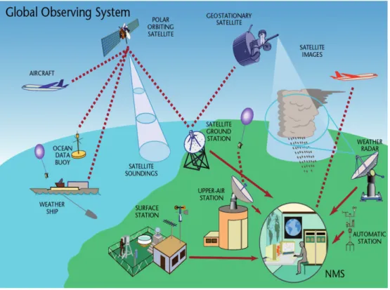
Meteorological observations made all over the world (Fig. 2.3) are used to compute the best estimate of the system initial conditions. Some of these observations, such as the ones from weather ballons or radiosondes, are taken at specific times at fixed locations (Fig. 2.4). Other data, such as the ones from aircrafts, ships or satellite, are not fixed in space. Thus the observa-tions used for the analysis of the atmosphere can be divided roughly into conventional, in-situ observations and non-conventional, remote-sensing ob-servations. The conventional observations consist of direct observations from surface weather stations, ships, buoys, radiosonde stations and aircraft, both at synoptic and, increasingly, at asynoptic hours. All surface and mean sea-level-pressure observations are used, with the exception of cloud cover, 2 m temperature and wind speed (over land). 2 m temperature and dew point

(32)

Figure 2.1: Grid points over Europe of ECMWF model (souce: ECMWF).

observations are used in the analysis of soil moisture. Observed winds are used from ships and buoys but not from land stations, not even from is-lands or coastal stations. The non-conventional observations are achieved in two different ways: passive technologies sense natural radiation emitted by the earth and atmosphere or solar radiation reflected by the earth and atmosphere; active technologies transmit radiation and then sense how much is reflected or scattered back. In this way surface-wind vector information is, for example, derived from the influence of the ocean capillary waves on the back-scattered radar signal of scatterometer instruments (Hersbach and Janssen 2007). Generally speaking, there is a great variability in the den-sity of the observation network. Data over oceanic regions, in particular, are characterised by very coarse resolution.

(33)

Figure 2.2: Vertical levels of the ECMWF model in previous versions (source: ECMWF).

be modified in a dynamical consistent way to obtain a suitable data set. This process is usually referred to as data assimilation.

In the ECMWF model, for example, dynamical quantities as pressure and velocity gradients are evaluated in spectral space, while computations involving processes such as radiation, moisture conversion, turbolence are calculated in grid-point space. This combination preserves the local nature of physical processes and retains the superior accuracy of the spectral method

(34)

Figure 2.3: Type of observations used to estimate the atmosphere initial conditions in a typical day (source: ECMWF).

Figure 2.4: Map of radiosonde locations (source: ECMWF).

for dynamical computation.

(35)

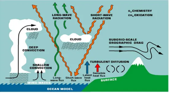
mix-ing, moist processes are active at smaller scales than the horizontal grid size. The approximation of unresolved processes in terms of model-resolved vari-ables is referred to as parameterisation (Fig. 2.5). The parameterisation of physical processes is probably one of the most difficult and controversial area of weather modelling (Holton 1992).

Figure 2.5: Schematic diagram of the different physical processes represented in the ECMWF model (source: ECMWF).

Nowadays, one of the most complex models used routinely for opera-tional weather prediction is the one implemented at the European Centre for Medium-Range Weather Forecasts (ECMWF). The starting point, in mathe-matical terms known as the initial conditions, of any numerical integrations is given by very complex assimilation procedures that estimate the state of the atmosphere by considering all available observations. The fact that a limited number of observations are available (limited compared to the degrees of free-dom of the system) and that part of the globe is characterized by a very poor coverage introduces uncertainties in the initial conditions. The initial condi-tions of a numerical weather prediction model can be estimated only within a certain accuracy. During a forecast some of these initial errors can amplify and result in significant forecast errors. Morover, the representation of the dynamics and physics of the atmosphere by numerical algorithms introduces

(36)

further uncertainties associated for instance with truncation errors, with un-certainty of parameters describing sub-grib scale processes such as cumulus convection in a global model. We will refer to these two kind of errors as ini-tial condition errors and model errors, respectively. For the prediction of the real atmosphere, these two kinds of errors are not really separable because the estimation of the initial conditions involves a forecast model and thus initial condition errors are affected by model errors. A requirement for ski-full predictions is for numerical models to be able to accurately simulate the dominant atmospheric phenomena. Computer resources contribute to limit the complexity and the resolution of numerical models and assimilation, as long as, in order to be useful, numerical predictions need to be produced within a resonable time limit.

These two sources of forecast errors generate weather forecast deteriora-tion with forecast time.

Initial conditions will always be known approximately, since each item of data is characterized by an error that depends on the instrumental accu-racy. In other words, small uncertainties related to the characteristics of the atmospheric observing system will always characterize the initial conditions. As a consequence, even if the system equations were well known, two initial states only slightly differing would depart one from the other very rapidly as time progresses (Lorenz 1965). Observational errors, usually in the smaller scales, amplify and through nonlinear interactions spread to longer scales, eventually affecting the skill of these later ones (Somerville 1979).

The error growth of the 10-day forecast of the ECMWF model was an-alyzed in great detail by Simmons et al. (1995). It was concluded that 15 years of research had improved substantially the accuracy over the first half of the forecast range (say up to forecast day 5), but that there had been little error reduction in the late forecast range. While this applied on average, it has also been pointed out that there had been improvements in the skill of the good forecast. In other words, good forecast had higher skill now, than before. The problem was that it was difficult to assess a-priori whether a forecast would be skillful or unskillful using only a deterministic approach to weather prediction.

(37)

Figure 2.6: The predictability problem may be explained in terms of the time evolution of an appropriate probability density function (PDF). Ensemble prediction based on finite number of deterministic integration seems to be a feasible method to predict the PDF beyond the range of linear growth (source: ECMWF).

Generally speaking, a complete description of the weather prediction problem can be stated in terms of the time evolution of an appropriate probability density function (PDF) in the atmosphere’s phase space (Fig. 2.6). Although this problem can be formulated exactly through the continu-ity equation for probabilcontinu-ity, ensemble prediction based on a finite number of deterministic integrations appears to be the only feasible method to predict the PDF beyond the range of linear error growth. Ensemble prediction pro-vided a way to overcome one of the problems highlighted by Simmons et al. (1995), since it can be used to estimate the forecast skill of a deterministic forecast, or, in other words, to forecast the forecast skill.

Since December 1992, both the US National Centre for Environmental Predictions (NCEP) and ECMWF have complemented their deterministic high-resolution prediction with medium-range ensemble prediction (Tracton & Kalnay 1993, Palmer et al. 1993). These developments followed the the-oretical and experimental work of, among others, Epstein (1969), Gleeson (1970), Fleming (1971a-b) and Leith (1974).

Both centres followed the same strategy of providing an ensemble of fore-casts computed with the same model, one started with unperturbed initial

(38)

conditions referred to as the ”control” forecast and the others with initial conditions defined adding small perturbations to the control initial condition (Fig. 2.7). Generally speaking, the two ensemble systems differ in the en-semble size, specifically in the fact that at NCEP a combination of lagged forecasts is used, and in the definition of the perturbed initial. The reader is referred to Toth & Kalnay (1993) for the description of the ’breeding’ method applied at NCEP and to Buizza & Palmer (1995) for a thorough discussion of the singular vector approach followed at ECMWF.

If forecast starting from perturbed analysis agrees more or less with the forecast from the non-perturbed analysis (the ensemble control forecast), then the atmosphere can be considered to be in a predictable state and any unknown analysis errors would not have a significant impact. In such a case, it would be possible to issue a categorical forecast with great certainty. On the other hand, if the perturbed forecasts (the ENSemble (ENS)) deviates significantly from the control forecast and from each other, it can be con-cluded that the atmosphere is in a rather unpredictable state. In this case, it would not be possible to issue a categorical forecast with great certainty. However, the way in which the perturbed forecast differs from each other may provide valuable indications of which weather patterns are likely to develop or, often equally importantly, not develop.

The ENS provides the ensemble mean (EM) forecast (or the ensemble median) where the less predictable atmospheric scales tend to be averaged out. In a well-costructed ensemble systems, the accuracy of the EM can be estimated a priori by the spread of the ensemble: the larger the spread, the larger the expected EM error, on average (Buizza, 2001). More importantly, the ENS provides information from which the probability of alternative de-velopments is calculated, in particular those related to high-impact weather.

The characteristics of a good ensemble are:

• The ensemble forecasts should display no mean errors (bias), otherwise the probabilities will be biased as well;

• The forecasts should have the ability to span the full climatological range, otherwise the probabilities will either over-or under-forecast the

(39)

Figure 2.7: Schematic of a probabilistic weather forecast using initial con-dition uncertainties. The blu lines show the trajectories of the individual forecasts that diverge from each other owing to uncertainties in the initial conditions and in the representation of sub-grib scale processes in the model. The main goal is to explore all the possible future states of the atmosphere. The dashed, lighter blue envelope represents the range of possible states that the real atmosphere could encompass and the solid, dark blue envelope repre-sents the range of states sampled by the model predictions. A good forecast is the one which analysis lies inside the ensemble spread (source: ECMWF).

risks of anomalous or extreme weather events.

Therefore, numerical weather prediction is, by its very nature, a disci-pline that has to deal with uncertainties. Over the past 15 years, ensemble forecasting became established in numerical weather prediction centres as a response to the limitations imposed by the inherent uncertainties in the prediction process. The ultimate goal of ensemble forecasting is to predict qualitatively the probability density of the state of the atmosphere at a fu-ture time. This is a nontrivial task because the actual uncertainty depends on the flow itself and thus varies from day to day.

(40)

2.2 The Lorenz system

Chaos Theory is a mathematical theory that can be used to explain com-plex systems such as weather. Although many comcom-plex systems appear to behave in a random manner, chaos theory shows that, in reality, there is an underlying order that is difficult to see. Many complex systems can be better understood through the lens of Chaos Theory. Henri Poincar´e laid the groundwork for Chaos Theory. He was the first to point out that many deterministic systems display a sensitive dependence on initial conditions. Later, in the 1900s, Edward Lorenz (1963, 1965) studied Chaos Theory in the context of weather systems. When making weather predictions, he no-ticed that his calculations were significantly impacted by the extent to which he rounded his numbers. The end result of the calculation was significantly different when he used a number rounded to three digits as compared to a number rounded to six digits. His observations on Chaos Theory in weather systems led to his famous talk, which he entitled, ”Predictability: does the flap of a butterfly’s wings in Brazil set off a tornado in Texas?”. Lorenz chaos model equations are:

     ˙ X =_{−σX + σY} ˙ Y =_{−XY + rX − Y} ˙ Z = XY _{− bZ}

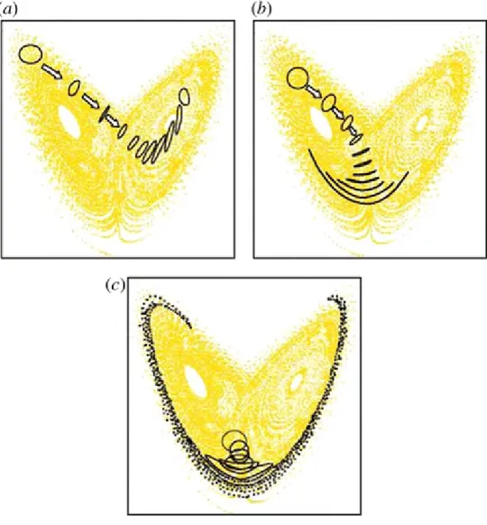
where σ is called the Prandtl number and r is called the Rayleigh number. All σ, r, b > 0, but usually σ = 10, b=8/3 and r is varied. The parameters σ, r, b are kept constant within an integration, but they can be changed to create a family of solutions of dynamical system defined by the differential equations. The particular parameter values chosen by Lorenz (1963) were: σ = 10, b=8/3 and r=28 -which result in chaotic solutions (sensitivity dependence on the initial conditions). Results from 3-dimensional Lorenz system illustrate the dispersion of finite time integrations from an ensemble of initial conditions (Fig. 2.8). The different initial points can be considered as estimates of the ”true” state of the system (which can be thought of as any point inside the ellipsoid) and the time evolution of each of them as possible forecasts. Subject to the initial ”true” state of the system, points close together at

(41)

initial time diverge in time at different rates. Thus, depending on the point chosen to describe the system time evolution, different forecasts are obtained.

Figure 2.8: Lorenz attractor with superimposed finite-time ensemble integra-tion (source: ECMWF).

The two wings of the Lorenz attractor can be considered as identifying two different weather regimes, for example one warm and wet and the other cold and sunny. Suppose that the main purpose of the forecast is to predict whether the system is going through a regime transition. When the system is in a predictable initial state (Fig. 2.8(a)), the rate of forecast divergence is small and all the points stay close together untill the final time. Whatever

(42)

the point chosen to represent the initial state of the system, the forecast is characterised by a small error and a correct indication of a regime transition is given. The ensemble of points can be used to generate probabilistic forecast of regime transitions. In this case, since all points end in the other wing of the attractor, there is a 100% probability of regime transition. By contrast, when the system is in a less predictable state (Fig. 2.8(b)), the points stay close together only for a short time period and then start diverging. While it is still possible to predict with a good degree of accuracy the future forecast state of the system for a short time period, it is difficult to predict whether the system will go through a regime transition in the long forecast range. Fig. 2.8(c) shows an even worse scenario, with points diverging even after a short time period and ending in very distant part of the system attractor. In probabilistic terms, one could have only predicted that there is 50% chance of the system undergoing a regime transition. Morover, the ensemble of points indicates that there is a greater uncertainty in predicting the region of the system attractor where the system will be at final time in the third case (Fig. 2.8(c)).

The comparison of the points’ divergence during the three cases indicates how ensemble prediction systems can be used to ”forecast the forecast skill” (Tennekes et al., 1986). In the case of the Lorenz system, a small divergence is associated to a predictable case and confidence can be attrached to any of the single deterministic forecasts given by the single points. By contrast, a large diverge indicates low predictability.

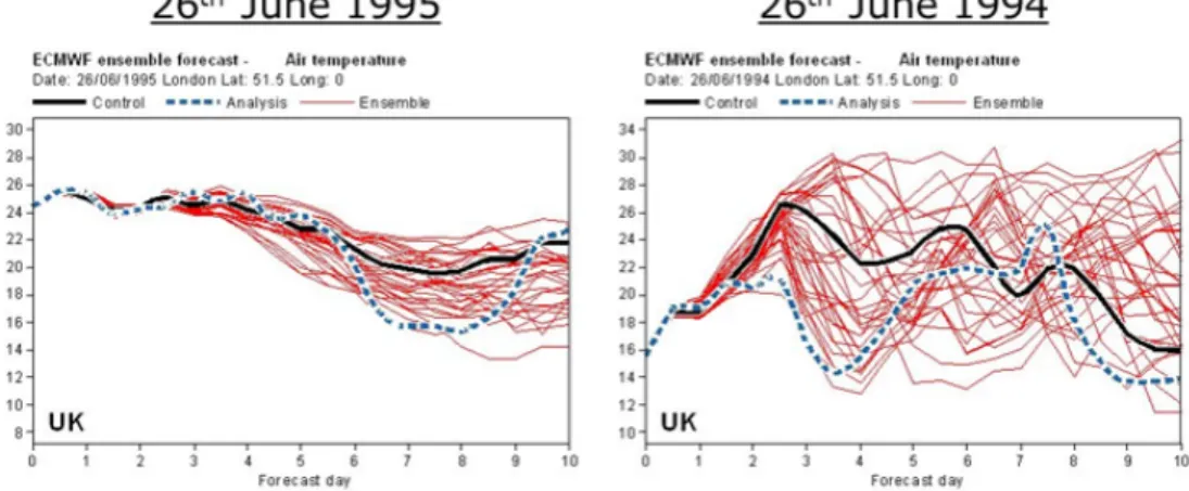
Similar sensivity to the initial state is shown in weather prediction. Fig. 2.9 shows the forecasts for air temperature in London given by 33 different forecasts started from very similar initial conditions for two different dates, the 26th _{of June of 1995 and the 26}th_{of June of 1994; in practice the image is}

about forecasts in the same place, one year apart. There is a clear difference degree of divergence during the two cases. All forecasts stay close together up to forecast day 10 for the first case (Fig. 2.9(a)), while they all diverge already at forecast day 3 in the second case (Fig. 2.9(b)). The level of spread among the different forecast can be used as a measure of the predictability of the two atmospheric states.

(43)

Figure 2.9: ECMWF forecasts for air temperature in London started from (a) 26 June 1995 and (b) 26 June 1994 (source: ECMWF).

2.3 Representation of model error

It has been already mentioned that uncertainties in the initial conditions and in the model are both sources of forecast error. Results from Harrison et al. (1999) indicate that the impact of model uncertainties on forecast error cannot be neglected. These results suggest that an ensemble system should try to describe not only the presence of uncertainties in the initial conditions, but also of model uncertainties. There is significant source of random error associated with the parameterized physical processes.

The laws of evolution which govern weather and climate, at least their physical aspects, are well known and are accurately represented by sets of partial differential equations. These equations nonlinearly couple circulta-tions with different scales and are thus difficult to solve analytically. To solve the governing equations numerically, we project them onto some cho-sen orthonormal basis, thus determining a set of (up to 108_{) coupled}

ordi-nary differential equations. Within these equations, the nonlinear effect of unresolved scales of motion are traditionally represented by simplified de-terministic formulae, known as parameterisations (Leutbecher and Palmer, 2007). These parameterisations represent the bulk effect of subgrid processes within a grid box and are justified in much the same way diffusive formulae are justified in statistical mechanics. Hence, for example, parameterisation

(44)

of deep convection assumes the existence of an ensemble of deep convective plumes, in quasi-equilibrium with the larger scale environment. The asso-ciated parameterised convective tendency represents the bulk effect of these plumes in redistributing heat, momentum and water in the vertical column of a given grid box. Similarly, parameterisation of orographic gravity-wave drag assumes the existence of an ensemble of incoherent gravity waves which collectively are associated with a flux of momentum from the surface to some level of wave breaking.

Parameterisations are by their nature approximations. Hence the pa-rameterised convective or orographic tendencies, which represent the mean effect of these processes over many realisations, are usually different from the tendencies associated with the actual convective or orographic subgrid flow. Since the latter is not known, the parameterisation process is nec-essarily a source of uncertainty in numerical forecasts and must therefore be represented explicitly in any ensemble forecast system. Without such a source of uncertainty either the ensemble will be underdispersive, or other sources of error, e.g. associated with observational uncertainty, will have to be inflated to prevent underdispersion. In this context, we note again that since the forecast model is used to assimilate observations in generating the initial conditions for a forecast, initial error includes a component due to model error. That is to say, when one speaks of forecast uncertainty as in-cluding initial error and model error, these two classes of errors are strictly interconnected.

There are several approaches to represent model errors: among them the most noticeable are the multi-model ensemble, the perturbed parameter ensemble and stochastic-dynamic parameterisation.

(45)

Chapter 3 Global and limited-area

ensemble prediction systems

This chapter describes three ensemble systems with different characteristics that will be subjected to a careful verification work in this thesis. These are ECMWF ENS, COSMO-LEPS and COSMO-2I-EPS, whose performance will be evaluated in chapter 5, on the basis of a week of observed data.

3.1 The ECMWF global atmospheric model

The ECMWF Integrated Forecasting System (IFS) consists of several com-ponents: an atmospheric general circulation model, an ocean wave model, a land surface model, an ocean general circulation model and perturbation models for Data Assimilation (EDA) and forecast (ENS) ENSemble, produc-ing forecasts from days to weeks and months ahead (ECMWF Forecast User Guide). The atmospheric general circulation model describes the dynamical evolution on the resolved scale and is augmented by the physical parameter-isation, describing the mean effect of subgrid processes and the land-surface model. Coupled to this is an ocean wave model (Bechtold et al. 2008).

3.1.1 The IFS equations

The model formulation is based on a set of basic equations, of which some are diagnostic, describing the static relationship beetween pressure, density,

(46)

temperature and height, and some are prognostic, describing the time evolu-tion of the horizontal wind components, surface pressure, temperature and the water vapour contents of an air parcel. Additional equations describe changes in the hydrometeors (rain, snow, liquid water, cloud ice content etc). There are options for passive tracers such as ozone. The processes of radiation, gravity wave drag, vertical turbolence, convection, clouds and surface interaction are, due to their relatively small scales (unresolved by the model’s resolution), described in a statistical way as parameterization pro-cesses (arranged in entirely vertical columns). Following Ritchie (1988, 1991), the first step in developing a semi-Lagrangian version of the ECMWF spec-tral model was to convert the existing Eulerian ζ _{− D (vorticity-divergence)} model to a U _{− V formulation, where U and V are the wind images defined} by U = u cos θ, V = v cos θ (u and v are components of the horizontal wind in spherical coordinates, and θ is latitude). We describe the Eulerian U _{− V} model. First we set out the continuous equations in (λ, θ, η) coordinates, where λ is longitude and η is the hybrid vertical coordinate introduced by Simmons and Burridge (1981). Therefore η(p, ps) is a monotonic function of

the pressure p and also depends on the surface pressure psin such a way that

η(0, ps) = 0 and η(ps, ps) = 1

The momentum equations are ∂U ∂t + 1 a cos2_θU ∂U ∂λ + V cos θ ∂U ∂θ + ˙η ∂U ∂η −fV + 1_a∂φ_∂λ + RdryTV ∂ ∂λ(ln p) = PU + KU (3.1) ∂V ∂t + 1 a cos2_θU ∂V ∂λ + V cos θ ∂V ∂θ + sin θ(U 2_{+ V}2_{) + ˙}_η∂V ∂η +f U + cos θ a ∂φ ∂θ + RdryTV ∂ ∂θ(ln p) = PV + KV (3.2)

where a is the radius of the earth, ˙η is the η-coordinate vertical velocity ( ˙η = ∂η_∂t), φ is geopotential, Rdry is the gas constant for dry air and TV is the

virtual temperature defined by

(47)

where T is temperature, q is specific humidity and Rvapis the gas constant for

water vapour. PU and PV represent the contributions of the parameterized

physical processes, while KU and KV are the horizontal diffusion terms. The

thermodynamic equation is ∂T ∂t + 1 a cos2_θU ∂T ∂λ + V cos θ ∂T ∂θ + ˙η ∂T ∂η − kTVω (1 + (δ_{− 1)q)p} = PT + KT (3.3) where k = Rdry

c_pdry (with cpdry the specific heat of dry air at constant pressure),

ω is the pressure-coordinate vertical velocity (ω = ∂p_∂t) and δ = c_cpvap

pdry (with

cpvap the specific heat of water vapour at constant pressure). The moisture

equation is ∂q ∂t + 1 a cos2_θU ∂q ∂λ + V cos θ ∂q ∂θ + ˙η ∂q ∂η = Pq+ Kq (3.4)

In the momentum equations, there is no vertical velocity, which therefore is not a prognostic variable of the model, but is diagnostic. In (3.2) and (3.3), PT and Pqrepresent the contributions of the parametrized physical processes,

while KT and Kq are the horizontal diffusion terms. The continuity equation

is ∂ ∂t( ∂p ∂η) +∇ · (vH ∂p ∂η) + ∂ ∂η( ˙η ∂p ∂η) = 0 (3.5)

where _{∇ is the horizontal gradient operator in spherical coordinates and} VH = (u, v) is the horizontal wind. The geopotential φ, which appears in

(3.1) and (3.2), is defined by the hydrostatic equation ∂φ ∂η =− RdryTV p ∂p ∂η (3.6)

while the vertical velocity ω in (3.3) is given by

ω = ₋ Z η 0 ∇ · (vH ∂p ∂η) dη +vH · ∇p (3.7)

This equation for verical velocity is diagnostic: ω is obtained from the diver-gence of the horizontal wind. In this ensemble system the vertical equation is approximated with the hydrostatic equation, therefore it is possible define

(48)

this model as hydrostatic. Expression for the rate of change of surface pres-sure and for the vertical velocity ˙η, are obtained by integrating (3.5), using the boundary conditions ˙η at η = 0 and at η = 1

∂pS ∂t =− Z 1 0 ∇ · (vH ∂p ∂η) dη (3.8) ˙ η∂p ∂η =− ∂p ∂t − Z η 0 ∇ · (vH ∂p ∂η) dη (3.9)

Since we use ln(ps) rather than ps as the surface pressure variable, it is

convenient to rewrite (3.8) as ∂ ∂t(ln ps) = − 1 ps Z 1 0 ∇ · (v H ∂p ∂η) dη (3.10)

3.1.2 The numerical formulation

The model equations are discretized in space and time and solved numerically by a semi-Lagragian advection scheme. This ensures stability and accuracy, using a time-step as large as possible to progress the computation of the forecast within an acceptable time. For the horizontal representation a dual representation of spectral components and grid points is used. All fields are described in grid point space. Due to the convergence of meridians, com-putational time can be saved by applying a ”reduced Gaussian grid”. This keeps the east-west separation between points almost constant by gradually decreasing the number of grid points towards the poles at every latitude in the extra-tropics. This also prevents the development of large gradient at high latitudes. For the computation of horizontal derivatives, a spectral rep-resentation, based on a series expansion of spherical harmonics, is used for a subset of the prognostic variables. The vertical resolution is the finest in ge-ometric height in the planetary boundary layer and the coarsest close to the model top. The ”σ-levels” follow the earth’s surface in the lower-most tropo-sphere, where the Earth’s orography displays large variations. In the upper stratosphere and lower mesosphere there are surfaces of constant pressure with a smooth transition in between (ECMWF Forecast User Guide).

(49)

3.1.3 Topographical and climatological fields

The model orography is derived from a data set with a resolution of about 1 km which contains values of the mean elevation above the mean sea level, the fraction of land and the fractionale cover of different vegetation types. These detailed data are aggregated (”upscaled”) to the coarser model resolu-tion. The resulting mean orography contains the values of the mean elevation above the mean sea level. In montainous areas it is supplemented by sub-grib orographic fields, to enable the parametrization of the effects of gravity waves and to provide flow-dependent blocking of air flow. For example, cold air drainage in valleys makes the cold air effectively ”lift” the orography. The land-sea mask is a geographical field that contains the percentage of land and water between 0 (100% sea) and 1 (100% land) for every grid point. A grid point is defined as a land point if its value indicates that more than 50% of the area within the grid-box is covered by land. The albedo is deter-mined by a combination of background monthly climate fields and forecast surface fields (e.g. from snow depth). Continental, maritime, urban and desert aerosols are provided as monthly means from data bases derived from transport models covering both the troposphere and the stratosphere. Soil temperatures and moisture in the ground are prognostic variables. There is a lack of observational data, so observed 2m temperature and relative humidity act as very efficient proxy data for the analysis. The snow coverage depth is analysed every six hours from snow-depth observations, satellite snow extent and a snow-depth background field. The snow temperature is also analysed from satellite estimates. They are forecast variables. Sea Surface Tempera-ture (SST) and ice concentration are based on analyses received daily from the Met Office (OSTIA, 5km). It is updated during the model integration, according to the tendency obtained from climatology. The temperature at the ice surface is variable and calculated according to a simple energy bal-ance/heat budget scheme, where the SST of the underlying ocean is assumed to be -1.7o_{C. The sea-ice cover, which is kept constant in the 10-day forecast}

integration, is relaxed towards climatology between days 10 and 30, with a linear regression. Beyond day 30 the sea-ice concentration is based on

(50)

cli-matological values only (from the ERA 1979-2001 data) (ECMWF Forecast User Guide).

3.1.4 The formulation of physical processes

Many physical processes occur at horizontal scales which are not resolved in the model. Their ”bulk effect” is expressed in terms of resolved model variables by parametrisation schemes. This involves both statistical methods and simplified mathematical-physical models such as adjustment processes. For example, the air closest to the earth’s surface exchanges heat with the surface through turbolent diffusion or convection, which adjusts unstable air towards neutral stability (Jung et al. 2010). The convection scheme does not predict individual convective clouds, only their overall physical effect on the surrounding atmosphere, in terms of latent heat release, precipitation and the associated transport of moisture and momentum. The scheme differentiates between deep, shallow and mid-level convection. Only one type of convection can occur at any given grid point at one time (see Fig. 3.1).

As for clouds, both convective and non-convective clouds are handled by explicit equations for cloud water, ice and cloud cover. Liquid and frozen precipitation are strongly coupled to other parameterized processes, in par-ticular the convective scheme and the radiation. The scheme also takes into account important clouds processes, such as the clouds that form in the low-est model level. The radiation spectrum is divided into a long-wave part (thermal) and a short-wave part (solar radiation). Since it has to take the cloud-radiation interaction into account in considerable detail, it makes use of a cloud-overlap algorithm which calculates the relative placement of clouds across levels. For the sake of computational efficiency, the radiation scheme is called less frequently than the model time step on a reduced grid. Nev-ertheless, it accounts for a considerable fraction of the total computational time. For the precipitation and hydrological cycles both convective and strat-iform precipitation are included in the ECMWF model (ECMWF Forecast User Guide). Evaporation of the precipitation, before it reaches the ground, is assumed not to take place within the cloud, only in the cloud-free,

(51)

non-Figure 3.1: The ECMWF total convective rainfall forecast from 28 November 2010 12 UTC +30h. The convection scheme has difficulty in advecting win-tery showers inland over Scotland and northern England from the relatively warm North Sea. The convection scheme is diagnostic and works on a model column, so cannot produce large amounts of precipitation over the relatively dry and cold (stable) wintery land areas. In nature these showers succeed in penetrating inland through a convectively induced upper-level warm anomaly leading to large-scale lifting and saturation (source: ECMWF).

saturated air beside or below the model clouds. The melting of falling snow occurs in a thin layer of a few hungred metres below the freezing level. It is assumed that snow can melt in each layer, whenever the temperature exceeds 0o_{C. The cloud-overlap algorithm is also important for the ”life}

his-tory” of falling precipitation: from level-with-cloud to level-with-clear-sky and vice versa. The near-surface wind forecast displays severe weaknesses in some mountain areas, due to the difficulty in parameterizing the inter-action between the air flow and the highly varying sub-grid orography (see Fig. 3.2). As with many other sub-grid-scale physical processes that need to

(52)

be treated in simplified ways, this problem will ultimately be reduced when the air-surface interaction can be described explicitly, thanks to a higher and appropriate resolution. The system also produces wind-gust forecasts as part of post-processing (Balsamo et al. 2011).

Figure 3.2: MSLP and 10 m wind forecast from 2 March 2011 12 UTC +12h. The 10 m winds are unrealistically weak over the rugged Norwegian mountains. Value of 10 m/s might be realistic in sheltered valleys, but not on exposed mountain ranges (source: ECMWF).

3.1.5 Overview of the ECMWF Ensemble Prediction

System

The ECMWF ENS Prediction System (hereafter ENS) contains 51 members, an unperturbed control forecast and 25 pairs of twin forecast with positive and negative initial perturbations. This yields a total of 50 global

(53)

perturba-tions for 50 alternative analyses and forecasts. Therefore, consecutive mem-bers have pair-wise anti-symmetric perturbations. The anti symmetry may, depending on the synoptic situation and the distribution of the perturba-tions, disappear after one day or so, but they can occasionally be noticed 3-4 days into the perturbed forecasts. The horizontal resolution of the ENS is about 18 km, but it increases to 32 km after the 15th _{day of the}

fore-cast range; the vertical resolution is 137 levels, which divide the atmosphere into many layers up to the isobaric hight of 0.01 hPa. The ENS configura-tion can be considered as an attempt to simulate random model errors due to parametrized physical processes. It is based on the notion that random errors due to parameterized physical processes are coherent between the dif-ferent parameterization modules and have a certain coherence on the space and time scales represented by the model. The scheme assumes that the larger the parameterized tendencies, the larger the random error component. In the ENS, each ensemble member ej can be seen as the time integration

ej(t) =

Z t t=0

[A(ej, t) + Pj0(ej, t)] dt

of the perturbed model equations

∂ej/∂t = A(ej, t) + Pj0(ej, t)

starting from the perturbed initial conditions

ej(t = 0) = e0(t = 0) + δej(t = 0)

where A and P0 identify the contribution to the full equation tendency of the non-parameterized and parameterized physical processes. For each grid point x = (λ, φ, σ) (identified by its latitude, longitude and vertical hybrid coordinate), the perturbed parameterized tendency (of each state vector com-ponent) is defined as

P_j0(ej, t) = [1+ < rj(λ, φ, σ) >D,T]P (ej, t)

where P is the unperturbed diabatic tendency and < _{· · · >}D,T indicates

(54)

DxD degree box and over T time steps. The notion of space-time coherence assumes that the organized systems have some intrinsic space and time-scales that may span more than one model time step and more than one model grid point. Making the stochastic uncertainty proportional to the tendency is based on the concept that the stronger organization (away from the notion of a quasi-equilibrium ensemble of sub-grid processes) is likely to be, the stronger is the parameterized contribution. A certain space-time correlation is introduced in order to have tendency perturbations with the same spatial and time scales as observed organization. The performance of the EPS has improved steadily since it became operational in the mid 1990s, as shown in Fig.3.3.

Figure 3.3: A skill measure for forecasts of the 850 hPa temperature over the northern hemisphere (20o-90oN) at days 3, 5 and 7. Comparing the skill measure at the three lead times demonstrates that on average the perfor-mance has improved by two days per decade. The level of skill reached by a 3-day forecast around 1998/99 (skill measure = 0.5) is reached in 2008/09 by a 5-day forecast. In other words, today a 5-day forecast is as good as a 3-day forecast 10 years ago. The skill measure used here is the Ranked Probability Skill Score (RPSS), which is 1 for a perfect forecast and 0 for a forecast no better than climatology (from ECMWF User Guide).