Facoltà di Ingegneria Industriale
Dipartimento di Scienze e Tecnologie Aerospaziali
M.S. in Aeronautical Engineering
A SOFTWARE MODEL FOR ROTORCRAFT FLIGHT
CONTROL SYSTEM ANALYSIS AND SIMULATION
Advisor: Prof. Giorgio Guglieri Advisor: Prof. Pierangelo Masarati
Student: Matteo Brighenti 764252
I would like to thank Prof. Giorgio Guglieri and Prof. Pierangelo Masarati for their support and brilliant insights. In addition, all friends and colleagues I have met here in Milan and all my friends in Brenzone. In conclusion, I would like to thank my Family for the support through my entire academic experience, which turned me into man and engineer; and especially thank to you, Zeno.
The flight control system (FCS) is the most important avionic component of a rotorcraft. It is deeply integrated with the other systems on board and has a huge impact on performances, flying qualities and especially safety. The design of this system is not easy and needs frequent design reviews. The case of this study is a fly-by-wire flight control system. The pilot’s control inputs are processed and electric signals are sent to the flight control surface actuators without any mechanical linkage.
The focus is on a mathematical model of the helicopter Sikorsky UH-60A Black Hawk [1] that is presented in the form of a block diagram. This model uses a modular architecture. Each module represents a single component of the FCS and has been studied and modified for this project. The software has been implemented and tested using for the campaign a state space model of the helicopter MBB Bo-105 and the parameters that configure the flight control system have been identified. The validation compares the data from the simulations with flight test data of the Bo-105 using doublet inputs on the three main axes controls during steady state horizontal flight.
The aim of this work is to develop a software model of a FCS for rotorcrafts that can be easily modified tuning few parameters and be used to investigate the flight behaviour of a rotorcraft due to this important component.
The use of a PID controller in place of the original system control blocks allows a quick tuning, while the modular architecture permits selective interventions that influence the motion around the single axes of the rotorcraft. Different sets of use of this component can be identified with the corresponding parameters of influence, to compose a library of the working points of the FCS.
Il flight control system (FCS) è il più importante componente avionico di un elicottero. E’ molto integrato con gli altri sistemi di bordo ed ha un forte impatto sulle prestazioni, le caratteristiche di volo e specialmente la sicurezza. Il progetto di questo sistema non è semplice e richiede frequenti revisioni. Il caso di studio qui presentato è un fly-by-wire flight control system: gli input di controllo del pilota sono processati e segnali elettrici sono inviati agli attuatori delle superfici di controllo del volo senza alcun collegamento meccanico.
L’attenzione è concentrata su un modello matematico del flight control system dell’elicottero Sikorsky UH-60A Black Hawk [1], presentato nella forma di schema a blocchi. Questo modello presenta una struttura modulare, in cui ogni modulo rappresentante i singoli componenti dell’FCS è stato studiato e modificato per questo progetto. Il software è stato quindi implementato e testato usando per questa campagna un modello agli stati dell’elicottero MBB Bo-105 ed i parametri importanti per configurare il flight control system sono stati identificati. La validazione è stata quindi portata avanti comparando i dati della simulazione con i dati derivanti da alcuni test in volo del Bo-105 usando come ingressi delle doppiette sui comandi dei tre assi principali partendo da una condizione di volo orizzontale uniforme.
Lo scopo di questo lavoro è quello di sviluppare un modello software di un FCS per elicotteri che può essere modificato con facilità tarando alcuni parametri e utilizzato per investigare il comportamento in volo di un elicottero in funzione di questo importante componente. L’utilizzo di un regolatore PID al posto dei blocchi di controllo del sistema originale permette una regolazione veloce del sistema, mentre la sua modularità consente interventi e modifiche puntuali che influenzano il moto sui singoli assi dell’elicottero. Possono quindi essere individuate diverse modalità di utilizzo con i corrispondenti parametri che le influenzano, andando a definire una libreria dei punti di lavoro dell’FCS.
List of Figures ... VII List of Tables ... IX List of Acronyms ... X 1 INTRODUCTION ... 1 -1.1 FCS OVERVIEW ... - 1 - 1.2 BLACK HAWK FCS ... - 3 - 2 MATHEMATICAL MODEL ... 4 -2.1 SENSORS ... - 7 -
2.2 STABILITY AUGMENTATION SYSTEM ... - 7 -
2.2.1 PITCH SAS CHANNEL ... - 9 -
2.2.2 ROLL SAS CHANNEL ...- 10 -
2.2.3 YAW SAS CHANNEL ...- 11 -
2.2.4 SAS NETWORK ...- 13 -
2.3 FLIGHT PATH STABILIZATION ...- 14 -
2.3.1 FPS PITCH CHANNEL ...- 15 -
2.3.2 FPS ROLL CHANNEL ...- 16 -
2.3.3 FPS YAW CHANNEL ...- 17 -
2.4 PITCH BIAS ACTUATOR ...- 18 -
2.5 MECHANICAL CONTROL SYSTEM ...- 19 -
2.6 STATE SPACE MODEL ...- 24 -
3 SIMULATIONS AND RESULTS ... 26
-3.1 PITCH CONTROL ...- 30 -
3.2 ROLL CONTROL ...- 35 -
3.3 YAW CONTROL ...- 40 -
4 CONCLUSIONS AND FUTURE DEVELOPMENTS ... 45
APPENDICES ... 46
-SIKORSKY UH-60A BLACK HAWK ...- 46 -
List of Figures
Figure 1 Complete FCS model ... 6
Figure 2 Pitch SAS channel ... 9
Figure 3 Roll SAS channel ... 10
Figure 4 Yaw SAS channel ... 12
Figure 5 SAS network ... 13
Figure 6 Pitch FPS channel ... 15
Figure 7 Roll FPS channel ... 16
Figure 8 Yaw FPS channel ... 17
Figure 9 PBA ... 18
Figure 10 Collective control ... 20
Figure 11 Lateral cyclic control ... 21
Figure 12 Longitudinal cyclic control ... 22
Figure 13 Tail rotor collective control ... 23
Figure 14 State space model ... 25
Figure 15 Longitudinal input without scale factor ... 27
Figure 16 Longitudinal input with scale factor ... 28
Figure 17 Pitch control: inputs ... 30
Figure 18 Pitch control: longitudinal input ... 31
Figure 19 Pitch control: pitch rate... 32
Figure 20 Pitch control: Euler angle theta ... 32
Figure 21 Pitch control: roll rate ... 33
Figure 22 Pitch control: Euler angle phi ... 33
Figure 23 Pitch control: yaw rate ... 34
Figure 24 Pitch control: Euler angle psi ... 34
Figure 25 Roll control: inputs ... 36
Figure 26 Roll control: lateral input ... 36
Figure 27 Roll control: roll rate ... 37
Figure 28 Roll control: Euler angle phi ... 37
Figure 29 Roll control: pitch rate... 38
Figure 30 Roll control: Euler angle theta ... 38
Figure 31 Roll control: yaw rate ... 39
Figure 32 Roll control: Euler angle psi ... 39
Figure 34 Yaw control: pedal input ... 41
Figure 35 Yaw control: yaw rate ... 42
Figure 36 Yaw control: Euler angle psi ... 42
Figure 37 Yaw control: roll rate ... 43
Figure 38 Yaw control: Euler angle phi... 43
Figure 39 Yaw control: pitch rate ... 44
Figure 40 Yaw control: Euler angle theta ... 44
Figure 41 Sikorsky UH60A Black Hawk ... 47
Figure 42 MBB Bo105 ... 49
Figure 43 Original pitch SAS channel... 50
Figure 44 Original roll SAS channel ... 51
Figure 45 Original yaw SAS channel ... 52
Figure 46 Original pitch FPS channel ... 53
Figure 47 Original roll FPS channel ... 54
Figure 48 Original yaw FPS channel ... 55
Figure 49 Original PBA ... 56
Figure 50 Original collective control ... 57
Figure 51 Original lateral cyclic control ... 58
Figure 52 Original longitudinal cyclic control ... 59
Figure 53 Original tail rotor collective control ... 60
Figure 54 Pitch control: velocity u ... 61
Figure 55 Pitch control: velocity v ... 62
Figure 56 Pitch control: velocity w ... 62
Figure 57 Roll control: velocity u ... 63
Figure 58 Roll control: velocity v ... 64
Figure 59 Roll control: velocity w ... 64
Figure 60 Yaw control: velocity u ... 65
Figure 61 Yaw control: velocity v ... 66
-List of Tables
Table 1 SAS pitch PID parameters ... 9 Table 2 SAS roll PID parameters ... 10 Table 3 SAS yaw PID parameters... 11
-List of Acronyms
FCS Flight Control System
SAS Stability Augmentation System
SCAS Stability Control Augmentation System ASE Automatic Stabilization Equipment FPS Flight Path Stabilization
PBA Pitch Bias Actuator FC Flight Computer
FCC Flight Control Computer
PID Proportional–Integral–Derivative MBB Messerschmitt-Bölkow-Blohm
1 INTRODUCTION
1.1 FCS OVERVIEW
The pilot must use three major controls in a helicopter during flight. They are the collective pitch control, the cyclic pitch control, and the tail rotor collective control [6]. In addition, the pilot must also use the throttle control, which is usually mounted directly to the collective pitch control. The system that controls the flight is the FCS [5] [4] and provides the pilot with a means to control the flight safely and effectively throughout its flight envelope.
When studying mechanics of flight and flight control it is common practise to assume that the aircraft can be represented as a rigid body, defined by a set of body-axis coordinates. The rigid-body dynamics have six degrees of freedom, given by three translations along, and three rotations about, the axes. All forces and moments acting on the vehicle can be modelled within this framework. If we can control these forces and moments, then we have control on the translational and rotational accelerations, and hence its velocities, attitude and position. The FCS aims to achieve this control via the control surfaces and its primary functions are pitch, roll and yaw control.
Every flight vehicle contains sensors, which provide measures of changes in motion variables, which occur as the vehicle responds to the pilot’s command or as it encounters some disturbance. The signals from these sensors can be used to provide the pilot with a visual display, or they can be used as feedback signals for the FCS. Thus, the general structure of a FCS can be represented as a block system. The purpose of the controller is to compare the commanded motion with the measured motion and, if any discrepancy exist, to generate, in accordance with the required control law, the command signals to the actuator to produce the control surface deflections which will result in the correct control force or moment being applied. This, in turn, causes the aircraft or the helicopter to respond appropriately so that the measured motion and commanded motion are finally in correspondence.
In helicopters, the basis instability is such that the FCS has to provide both restoring and damping moments. However, only limited control authority can ever been allowed, since control is through the rotor which provides the helicopter sustaining lift and forward propulsion.
Part of the FCS is the stability augmentation system (SAS) [3], which augments the stability of the aircraft. It mostly does it by using the control surfaces to make the aircraft more stable. The SAS is always on when the aircraft is flying. Without it, the aircraft is less stable or possibly even unstable. It supplies short-term attitude and attitude rate stabilization for use in hands-on flying. It is referred to as an SAS because it stabilizes the helicopter against outside disturbances, and augments or helps pilot cyclic control input. The SAS is designed so that pilot controlled motions are enhanced while helicopter motions caused by outside disturbances are counteracted. This mode of operation improves basic helicopter handling qualities. The principal SAS functions are pitch rate SAS, yaw damper, roll rate damper and relaxed static stability SAS.
The stability control augmentation system (SCAS) [2] is a tool for the pilot to control the aircraft. The purpose of this system is to provide control of the helicopter. If this system is not present, the SAS would sense any disturbance in the helicopter from a control input, i.e. pilot or autopilot command, and damp it. Instead, the SCAS ‘feeds the signal forward’ which results in a delay of the damping. Without the SCAS the damping would take place immediately and the responsiveness of the helicopter would be slow at best.
Another common FCS subsystem is the automatic stabilization equipment (ASE) [2]. It is an attitude control system and allow the rotorcraft to be placed, and maintained, in any required, specified orientation in space. The input from the trim system centres the gyro for any given flight condition. A signal from the stick system is used to ‘break off’ the gyro signal produced. When the stick is trimmed to some new datum position, this signal establishes a new datum for the gyro. An ASE can hold attitude indefinitely.
Another level of control consists of the autopilot [2]. This autopilot works to maintain airspeed, altitude, and sideslip. While the helicopter is traveling forward there is some inherent sideslip, which means the helicopter, is not traveling in a straight line but at a slight diagonal. This system will maintain the height and sideslip according to the levels set by the autopilot.
In the early days of flying, the FCS was mechanical. By means of cables and pulleys, the control surfaces of the first aircrafts were given the necessary deflections to control the aircraft. The maximum levels of pilot’s stick and pedal forces required to manoeuvre a flight vehicle are limited by the physical capabilities of the pilot, which have not changed since the times of the Wright brothers. When aeroplanes evolved in size and speed, the forces to move the control surfaces against the aerodynamic forces grew to a point where they exceeded the capabilities of any pilot. This made additional power sources necessary: hydraulic boosters were first installed at the end of World War II. The next step was the introduction of fully power-operated controls with the removal of the direct connection between the pilot’s feel and control-surface forces. Later on, the role of the mechanical linkages between pilot’s cockpit controls and the hydraulic actuators was reduced to one of signalling, and no longer to transmit power. In the 70’s the fly-by-wire architecture was developed, starting as an analogue technique and later on, in most cases, transformed into digital. It was first developed for military aviation, where it is now a common solution. The supersonic Concorde can be considered a first and isolated civil aircraft equipped with a (analogue) fly-by-wire system, but in the 80’s the digital technique was imported from military into civil aviation by Airbus, first with the A320, then followed by A319, A321, A330, A340, Boeing 777 and A380.
In the fly-by-wire system electrical signals are sent to the control surfaces. The signals are sent by the flight (control) computer (FC/FCC). In this way, the aircraft is controlled. But what is the advantage of automatic flight control? There are several reasons for this. First, a computer has a much higher reaction velocity than a pilot and it is not subject to workload. Finally, a computer can more accurately know the state the aircraft is in.
The desire for further reduction of accident rates, new aircraft programmes, development of new technologies and improvements of the design process will drive the future FCS evolution. Fly-by-wire technology offers new opportunities to increase the overall level of safety. New technologies promises further improvements.
The integration of new functions or especially new air-traffic-control functions, which become possible with data links, will have an influence in future FCSs. A supersonic transport aircraft, which may be developed as a Concorde successor, presents new challenges for the FCS.
1.2 BLACK HAWK FCS
The Black Hawk’s FCS is an electro-hydro mechanical servo system employed to introduce improved control and stability characteristics and reduce pilot workload.
The flight control system defined in the simulation model is comprised of the following elements:
a) Sensors
b) Stability Augmentation System (SAS) c) Pitch Bias Actuator (PBA)
d) Flight Path Stabilization (FPS) e) Mechanical Controls
The sensors are the motion transducers, which provide feedback input to the FCS. The FCS main components are the SAS and the FPS.
The SAS system uses rate damping to improve dynamic stability and will be discussed in more detail in a later section. The FPS acts as the helicopter’s autopilot.
The FPS serves as the long-term memory and operates with 100% authority over the flight controls, at a limited rate, to maintain the pilot’s selected flight, such as heading hold and altitude hold.
The function of the PBA is to increase the static longitudinal stability.
The mechanical controls represent the collective control, the lateral cyclic control, the longitudinal cyclic control and the tail rotor collective control.
All the subsystems models were developed using SIMULINK®; but for the purposes of keeping the simulation less complicated, FPS and PBA were not implemented in the software. In particular PBA was not considered because it is an obsolete technology nowadays, considering that the UH-60 simulation program was delivered in 1981, and the FPS was not strictly necessary for this simulation given the pseudo attitude features of the SAS.
2 MATHEMATICAL MODEL
This thesis project is to initiate and take the first steps in the development of a flight simulation Black box tool. The simulation has been constructed using SIMULINK® and has been developed by modifying existing helicopter simulation block diagrams indicating the transfer function between signals of a Sikorsky engineering simulation program [1]. The operation of this tool will be initiated by inputting data into the SIMULINK® simulation via a MATLAB® set up file encoded with the helicopter specifications and possible engineering changes.
This thesis starts from the need to have an appropriate software library to study the behaviour of an FCS, its coupling with another rotorcraft and its impact over the entire system characteristics.
The system is composed of two main blocks that are independent and shares input and output data. The first block is the flight control system (FCS) block of the Sikorsky UH-60A Black Hawk that is composed of other blocks as well and the second one is a state space model of the MBB Bo-105. As required by specific problems the resulting intrinsic modularity of this software allows to easily incorporate improved features.
The FCS presented in this model covers the primary mechanical flight control system and the automatic flight control system. The control functions collectively enhance the stability and control characteristics of the helicopter. The analytical definition of the control system incorporates sensors, shaping networks, logic switching, authority limits and actuators. Every component of the system has been designed as a black box with inputs and outputs that connect the subsystems with each other and with the state space model. The design is entirely based on the Black Hawk Engineering Simulation Program [1] [7]. The original blocks of this program (that are shown in the appendices) were first studied extensively and all the single blocks functions and properties were determined and validated through simulations that are presented in the next chapter.
The SAS was modelled in accordance to the document without any modification. The analog and the digital pitch SAS channels present similar structures and are the same as the original ones. On the other hand, the analog and the digital roll SAS channels have different structures and different inputs. We wanted the system to have the same output from the two channels and a first study of this component via step response has demonstrated that they have slightly different outputs, while pitch SAS and yaw SAS output are virtually identical. However, the range between the two outputs is not significant enough to require a modification of the blocks. The yaw SAS channels uses switches piloted by velocity that were modelled although we consider a constant velocity throughout the simulations.
The FPS was modelled with some modifications. Once the trim position has been stored, the output of the synchronizer instantaneously goes to zero, which acts to normalize set points in the autopilot. The synchronizers than provide a signal indicative of the difference between the trim position and the current input value. In this project, the synchronizers (SYNC in the original document) were not modelled and the input is modified in order to be the difference
between the set point and the current state. Since we considered the helicopter in a steady flight condition we put the turn switch in the off mode and did not modelled it.
The state space model is considered in the usual form 𝑥̇ = 𝐴𝑥 + 𝐵𝑢, and the outputs are converted in the FCS units of measures, before being processed by the FCS.
The figure that follows in the next page shows the entire FCS system (not the state space model) with all its components and all the links between them, showing inputs and outputs. In the next pages the single subsystems are described.
2.1 SENSORS
These are the helicopter motion transducers, which provide feedback input to the FCS. They are represented in the simulation by high frequency second order transfer functions. Signal conditioning (6-7 Hz first order filter) is applied to all sensor outputs.
The sensors has not been modelled as subsystems, but they are inside the blocks, as transfer functions.
Rate gyros transfer function 0.00014𝑆[𝑑𝑒𝑔/𝑠𝑒𝑐]2+0.016𝑆+1
Lateral acceleration transfer function 0.0254𝑆[𝑓𝑡/𝑠𝑒𝑐2+0.233𝑆+12]
2.2 STABILITY AUGMENTATION SYSTEM
The SAS is a dual system comprised of an analog and a digital channel for each axis. The simulation definitions for pitch, roll and yaw SAS channels are shown on the figures below. Each figure incorporates the representation of the digital and analog SAS channels. In general, the helicopter motion sensed by the gyroscopes is passed through signal conditioning filters before being shaped by the SAS networks. The signal is then processed through a washout filter, if required, that makes transitions caused by changes in the input more smooth. Then there is a 2:1 gain change switch. The switch definition is ON/ON, both channels working at gain 1.0, 0N/OFF, only the digital channel works at gain 2.0; OFF/ON, only the analog channel works at gain 2.0. Finally, the signal is restricted in amplitude by a 5% authority limit. In the case of the digital channel, the signal is passed through zero order hold to account for update delays. It describes the signals as a discrete-time signal by holding a constant sample value for one sample interval. A switch in the yaw channel is a turn coordination aid, that is not studied in our simulation.
This system provides three rate damping and pseudo attitude retention channels:
Pitch SAS Channel
Roll SAS Channel
Yaw SAS Channel
It enhances the basic helicopter stability about the three main axes using rate feedback. During normal operation with both SAS engaged (digital and analog), each provides one half of system nominal gain and one half of total system control authority. The control authority of each is electrically limited to ±5 percent of total control travel in pitch, roll, and yaw. SAS inputs to the SAS servo valves are additive to provide a total authority of 10 percent. The sum is limited to ±10 percent authority by mechanical limits of SAS actuator travel. These two
channels can be selected separately on the Automatic Flight Control Panel. If one channel is selected off because of a failure, gain in the 'ON' channel is doubled but the authority remains at ±5 percent.
The modules were developed from the original document and then adapted for the Bo-105 state space model. Two important elements were introduced in the system:
PID controller in place of the original regulation blocks.
Scale factor K that considers the different inertial properties between the two helicopters considered.
In the following figures modifications are shown. In particular, the green boxes are the components sensitive to regulation that have been replaced with a PID (proportional– integral–derivative) controller. The light turquoise gains (that we will call factor K, shown afterwards) are the mathematical relationships of the square roots of the moments of inertia on each axis of the two helicopters taken in consideration. The Bo-105 has different characteristics from the UH-60A and this ratio is proportional to the ratio of the natural frequencies of the planes. Using this parameter the FCS is adapted to the mass and geometrical features of the Bo-105. The signal is scaled, preventing oscillation of the response. The tuning of the controller was then based upon flight test data of the MBB Bo-105 as we will see further in the next chapters.
The PID is in the form 𝑃𝐼𝐷 = 𝑃 + 𝐼1𝑆+ 𝐷 𝑁
1+𝑁 𝑆 𝐾 = √𝐽𝐵𝑜−105 𝐽𝑈𝐻−60𝐴 𝜔𝐵𝑜−105 𝜔𝑈𝐻−60𝐴
The control variables are given in %:
Longitudinal stick: -100% pushed, +100% pulled
Lateral stick: -100% left, +100% right
Pedal: -100% pushed left, +100% pushed right
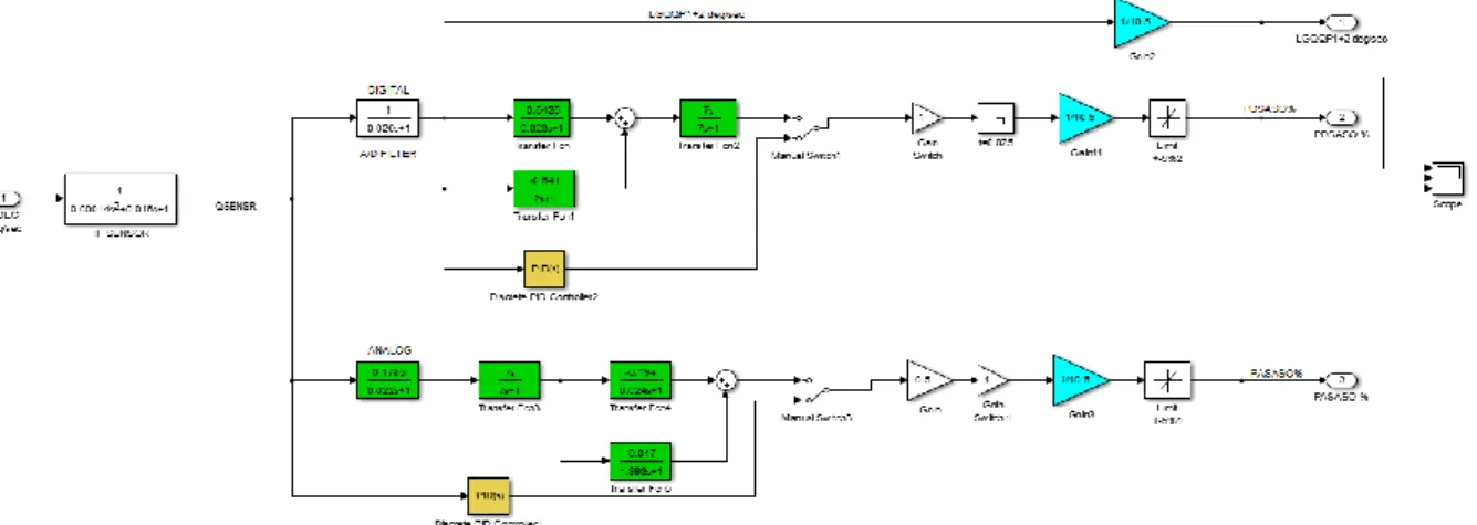
2.2.1 PITCH SAS CHANNEL
The input of the subsystem is the pitch rate QDEG (deg/sec) and the outputs are LGQQP1+2 (deg/sec), PDSASO and PASASO. PDSASO and PASASO (% of command) are the percentage of the command that is sent to the longitudinal cyclic control by the digital and the analog channel, LGQQP1+2 is a coupled parameter sent to the FPS pitch and to the PBA that work on the same axis.
PID DIGITAL P=-1.1 I=-0.194 D=0 PID ANALOG P=-2.128 I=-0.554 D=0 K=1/10.5
Table 1 SAS pitch: PID parameters
2.2.2 ROLL SAS CHANNEL
The inputs of the subsystem are the roll rate PDEG (deg/sec) and the bank angle PHIB (deg) for the digital channel, only the bank angle PHIB (deg) for the analog channel. The outputs RDSASO (%) and RASASO (%) are the signals sent to the lateral cyclic control by the digital and the analog channels. The output LGPPR1+2 is sent to the FPS roll, the FPS yaw and the SAS yaw subsystems, the output LGPHR2+2 (deg/sec) is sent to the SAS yaw. These are coupled parameters that influence yaw and roll; in fact, these two degrees of freedom outside the symmetry plane of the helicopter affect each other’s dynamics.
PID DIGITAL P=-0.381 I=-0.091 D=0 PID ANALOG P=-3.599 I=-1.795 D=0 K=1/4.41
Table 2 SAS roll PID parameters
2.2.3 YAW SAS CHANNEL
This SAS subsystem is different from the other two and has a more complex logic and more inputs. There are the yaw rate RDEG (deg/sec) and the lateral acceleration AYPS1 (ft/sec^2), the coupling terms LGPHR2+2 (deg/sec) and LGPPR1+2 (deg/sec) from the SAS roll channel and the velocity V (kts), that commands 4 switches (coloured grey in the block diagram that follows).
These switches define two regulation modes modifying the blocks connections in the same way in the digital and in the analog channels (if not clear in the next figure, it can be seen in the original diagram present in the appendices). If the velocity is below 60 kts the switches close downward. In this case, the control due to the rate input is augmented, and the contribution from the coupling terms and the lateral acceleration is cut off from the circuit. On the other hand, if the velocity is above 60 kts the switches close upwards. The coupling between the dynamics of the yaw and the roll angle become critical and is taken into consideration for the regulation in the circuit as much as the lateral acceleration, while the control due to the yaw rate reduces its impact. Since a steady flight at 80 kts is considered as initial condition for the simulations presented in here we will refer to the second case. The output signals YDASASO (%) and YASASO (%), respectively from the digital and the analog channel, are sent to the tail rotor collective control.
Furthermore, a coefficient in the determiner of the magenta block (see the block diagram) was changed from the original system. 0.0001s was replaced with 0.001s, because the frequency of this first order filter was too high for the computational capacity available for this work. This modification prevented the crash of the simulation and its impact on the results was considered negligible.This channel has been the most difficult to tune for the PID between the SAS ones, and it is the only one that present derivative action.
PID DIGITAL P=-0.78 I=-0.00048 D=-19.387 N=0.072 PID ANALOG P=-1.650 I=-0.001 D=-35.933 N=0.071 K=1/12.17
2.2.4 SAS NETWORK
The SAS subsystems are here presented for a visual recap of inputs, outputs and coupling terms inside the SAS (light blue and yellow), described in the previous paragraphs.
2.3 FLIGHT PATH STABILIZATION
This system provides three attitude retention channels:
Pitch FPS Channel
Roll FPS Channel
Yaw FPS Channel
The FFS shaping networks are relatively straightforward; however, a degree of complication is introduced by the automatic turn coordination capability. On the helicopter, several channels of complex logic enable the turn switch. Since the FPS is computed in the digital computer, the final output is passed through a zero order hold.
The FPS system provides the BLACK HAWK with outer loop stabilization through the pedals and the longitudinal and lateral stick actuators. The FPS can drive the cockpit control to any position to which the pilot can trim the controls, resulting in a 100 percent FPS parallel control authority, while the rate is limited at 10%/sec. The FCS limits the rate of FPS within the maximum override force limits. The attitude hold function of the FPS is designed to maintain pitch and roll attitude, plus a desired heading. The FPS presented in the Flight Control module identifies the FPS switch, and the turn switch. The FPS is activated by the pilot through a switch on the FCS panel.
The subsystem has been reconstructed, but not tuned, and is suitable for future developments. The outputs are scaled by the same factors used for the SAS considering the different features of the helicopters considered.
2.3.1 FPS PITCH CHANNEL
The input of the subsystem are LGQQP1+2 (deg/sec) from the SAS pitch channel, the pitch angle THETAB (deg) for the desired attitude and the velocity V (kts). The velocity takes part of the regulation above 30 kts. The signal is passed through a trim actuator closed loop which output is the percentage on the control. The percentage of control is then converted into inches of command XBOLS to the longitudinal cyclic control.
2.3.2 FPS ROLL CHANNEL
The input of the subsystem are LGPPR1+2 (deg/sec) from the SAS roll channel and the roll angle PHIB (deg) for the desired attitude. The signal is then processed as the FPS pitch channel with a trim actuator loop and a conversion of the signal. The output XAOLS (ins) goes to the later cyclic control.
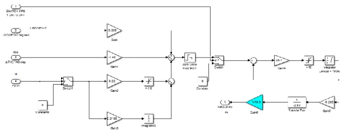
2.3.3 FPS YAW CHANNEL
This SAS subsystem is different from the other two and has a more complex logic and more inputs. The input of the subsystem are LGPPR1+2 (deg/sec) from the SAS roll channel, the desired heading PSIB (deg) for the desired attitude, the lateral acceleration AYPS1 (ft/sec^2), the velocity V (kts) and the collective stick position XCTOT (%). Beside the inputs, there is still a trim actuator loop and a conversion of the signal as in the other FPS channels. The output XPOLS (ins) goes to the tail rotor collective control.
2.4 PITCH BIAS ACTUATOR
The PBA representation is presented in the figure below. The input signals are derived as indicated: pitch angle THETAB (deg), airspeed V (kts), LGQQP1+2 (deg/sec) from the SAS pitch channel. Output is XBBAS (ins) to longitudinal cyclic control. The three input signals are limited, passed through a gain and summed to obtain the signal output to the PBA actuator. The actuator travel is restricted by a ±3%/sec rate limit and a 15% authority limit. Because the digital computer computes the PBA algorithm, the simulation includes a zero order hold. The PBA is an integral part of the BLACK HAWK control system. The pilot has no control switch for this system in the cockpit. The purpose of the PBA is to improve the apparent static longitudinal stability for the aircraft through attitude and airspeed feedback. The PBA is, in effect, a variable length controlled rod, which changes the relationship between longitudinal cyclic control and swashplate tilt, as a function of flight parameters. The attitude feedback covers the entire speed envelope. The airspeed feedback is only active between 80 and 180 knots. In addition to the attitude and airspeed feedback, pitch rate feedback is also present. Hence, there is also position feedback to the longitudinal stick proportional to pitch rate.
2.5 MECHANICAL CONTROL SYSTEM
In addition to its function as a mixing unit for control coupling, this part of the simulation is used to bring together the various elements of the control system computed upstream. The primary controls presented here are:
Collective control
Lateral cyclic control
Longitudinal cyclic control
Tail rotor collective control
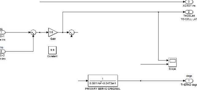
The longitudinal cyclic command is here used for purposes of discussion, while the other controls are slightly different. The outputs from the digital and analog SAS channels are summed and processed through the SAS actuator dynamics, resulting in actuator travel in inches (XBILS) This is summed with the PBA (XBBAS), the FPS (XBOLS) and the pilot control stick input (XB+2). The resultant linkage motion is converted into equivalent degrees of longitudinal cyclic before being summed with coupled motion from other controls in the mixing unit. The output from the mixing unit BISMIX is modified by the primary servo dynamics giving the final longitudinal cyclic impressed on the main rotor. The mechanical control system is designed to reduce pilot workload by coupling the controls to account for natural single rotor helicopter coupling responses to given control inputs.
2.6 STATE SPACE MODEL
The differential equations of motion of the MBB Bo-105, describing perturbed motion around the working point of the general trim condition, can be written as:
𝑥̇ = 𝐴𝑥 + 𝐵𝑢
Where x is the state vector:
𝑥𝑇 = (𝑢 𝑣 𝑤 𝑝 𝑞 𝑟 𝜑 𝜃 ψ 𝑝̇ 𝑞̇ 𝑟̇ )
Moreover, u is the control vector:
𝑢𝑇 = (𝑑𝑥 𝑑𝑦 𝑑0 𝑑𝑝 )
The state vector has 12 components:
• 𝑢 𝑣 𝑤 are the translational velocities along the three orthogonal directions of the body fixed axes system
• 𝑝 𝑞 𝑟 are the angular velocities around the x-, y- and z-axis
• 𝜑 𝜃 ψ are the Euler angles, defining the orientation of the body axes relative to the earth • 𝑝̇ 𝑞̇ 𝑟̇ are the angular accelerations around the x-, y- and z-axis
The positive orientations of the axes of the body fixed system are: • x pointing forward
• y pointing to the right • z pointing downward
The control vector with the pilot controls has four components, is given in percentage and is the output of the FCS:
• dx is the longitudinal pilot control: -100% pushed +100% pulled • dy is the lateral pilot control: -100% left +100% right
• d0 is the collective pilot control: 0% pushed down +100% pulled up • dp is the pedal pilot control: -100% pushed left +100% pushed right
The angles are expressed in radiant, the lengths in m and the velocities in m/sec^2. This data was transformed to be used in the FCS system that works with degrees, feet and kts. Using a derivation block in the simulation the lateral acceleration used in the FCS was found.
3 SIMULATIONS AND RESULTS
The simulations that have been performed concern the validation of the FCS and state space model integrated system and the tuning of the three axes SAS channels PID based on flight test data of the Bo-105.
After the reconstruction of all the FCS subsystems, that was difficult because of the poor quality of the documents and the lack of some information in the papers, the behaviour of the single subsystems was studied to verify the validity of some hypothesis we made. The first simulations dealt with the step response of the single SAS original subsystems on each axis separately, where the presence of the pseudo attitude retention features of the system were discovered, since the asymptotical response of the angular velocities was zero. At first, we studied separately the analog, the digital channels and then we tasted them together. Eventually we repeated the procedure using a sinusoidal and an impulse input.
After the system was considered stable, the next step was to engage the SAS with the mechanical control system, which works as a mixing unit, and the state space model. The control signals from the FPS, the SAS and the PBA are summed here with the pilot inputs, the trimmed conditions, and the coupling terms between the mechanical controls subsystems, to define the final command output to the state space model. All this signals are expressed in terms of inches of travel on the commands while the output angles refer to the aerodynamic angles of the UH-60A that are not the object of the simulations. The data is then converted from inches to percentage of command and the perturbation from the stable flight conditions are defined as inputs to the state space model that provides the perturbed motion around the working point of the general trim condition.
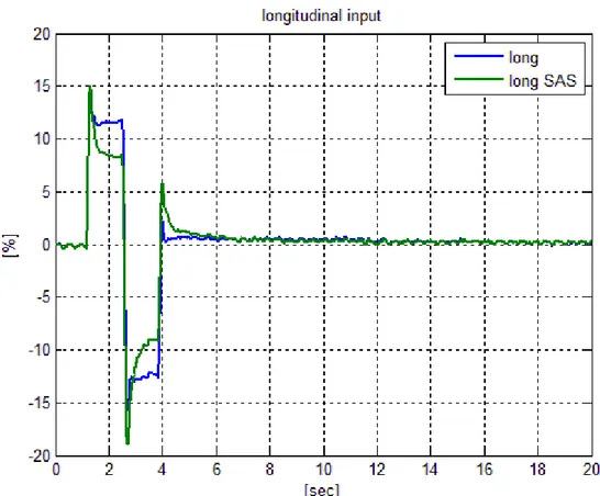
At this point, we studied the complete system. The task was to adapt the flight control system to a helicopter different from the one that it was designed for. We investigated the model response using doublets inputs on the longitudinal and later cyclic control, and on the tail rotor collective control. We used the same inputs of the flight tests of the Bo-105 and we compared the results. As we did before we implemented one SAS channel at the time. We started with the pitch SAS channel and with a doublet input on the longitudinal control. The response was oscillatory and the SAS system needed some modification. We introduced a scale factor K (previously discussed in paragraph 2.2) on the outputs of the SAS channel that adapted the system to the dynamics of the Bo-105 scaling the signals through the natural frequencies of the two rotorcraft. The scaling impact is shown in the following figures where we can see the different contribution of the SAS channel to the command (expressed in percentage of control) with and without the factor K. The blue graph represents the pilot input and the green graph the pilot input to the state space model through the mixing unit with the contribution of the SAS system, where:
long = longitudinal cyclic control input
long SAS = longitudinal cyclic control input with SAS engaged (in this case only the pitch SAS channel)
Figure 16 Longitudinal input with scale factor
We performed the same operation on the other two SAS channels, which showed the same behaviour, with the same results.
The aim of this simulation campaign was to have an output from the model similar to the flight test data. Once we gained the stability of the SAS, we compared the flight test data with the response of the state space model alone and the state space model with the SAS engaged (always using one SAS channel at the time). We could see the impact of the SAS on the state space model and obviously the perturbations were better dumped with the SAS and the response was closer to the flight test model. As indices of performance of the model we considered mostly the angular velocity respect to the command considered, and secondly the other components of the state. Eventually the three SAS channels were used together resulting in a further better response of the system overall; in particular the behaviour of the linear velocities was improved.
To improve further the system we introduced PID controllers in the SAS channels with appropriate tuning. We first located the regulation blocks of the original system and then we replaced them with the new controllers. We used the same procedure we performed in the other simulations. We tuned the regulators one by one, considering one channel at the time, investigating separately the digital and the analog channel. Then, we tested the analog and the digital channel together. Finally, we tested the complete SAS system with all the PID regulators and proceeded with the final tuning. The model output states complied with the flight test data and we noted the improvement of the linear velocities response using all the SAS channels together. The flight test of the Bo-105 were performed using doublet inputs on
the longitudinal and lateral cyclic and on the pedal control. We used the same inputs for the model and we will discuss next the results.
In each paragraph the first figure represents the relative variation of the input commands of the flight test data from the steady state conditions, where:
long = longitudinal cyclic control input
lat = lateral cyclic control input
coll = collective control input
pedal = tail rotor collective control
In the second figure, we can see the relative variation of the command on the axis that the doublet input is applied to, where:
long SAS = longitudinal cyclic control input with SAS engaged
lat SAS = lateral cyclic control input with SAS engaged
pedal SAS = tail rotor collective control with SAS engaged
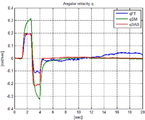
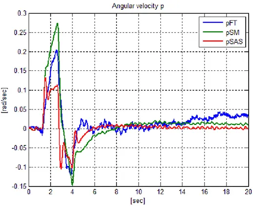
The other ones represent the rotational velocities around the three axes and the Euler angles. In blue we have the data of the flight tests, in green the response of the state space model alone, and in red the response of the state space model with the SAS engaged, where:
pFT pSM pSAS = pitch rate relative to flight tests, state space model and state space model + SAS
qFT qSM qSAS = roll rate relative to flight tests, state space model and state space model + SAS
rFT rSM rSAS = yaw rate relative to flight tests, state space model and state space model + SAS
phiFT phiSM phiSAS = Euler angle relative to flight tests, state space model and state space model + SAS
thetaFT thetaSM thetaSAS = Euler angle relative to flight tests, state space model and state space model + SAS
psiFT psiSM psiSAS = Euler angle relative to flight tests, state space model and state space model + SAS
The units of measure are:
Command inputs [% of command] as in the state space model chapter
Angular velocity [rad/sec]
Angle [rad]
3.1 PITCH CONTROL
In the first figure, we can see that there is some noise in the lateral cyclic control probably due to a little pilot error that is not considered significant. The doublet input on the longitudinal control starts after 1.2 seconds, and at 3.9 seconds the control is set back at the original position. The positive and the negative variations of the command are almost equal; they present two peaks at ±15% and stabilize around +11.6% and -12.5%.
The pitch rate response of the model (qSAS) is symmetric respect to the initial conditions, as the input, and is closed to the flight test results except for the negative peak of the angular velocity (-0.2 rad/sec). The reason is that the state space model response is symmetric to positive and negative variations, while the real model is not. This is clear because with the SAS engaged (qSAS) or not (qSM) we have the same symmetry. The SAS makes transitions smoother, cuts off the peaks of the pitch rate respect to the state space model (qSM), and gives a constant response to the input. Finally, the angular velocity of our model stabilizes at the null value quicker than in the flight test.
The angle theta (thetaSAS) reaches a peak and then stabilizes quickly damping the oscillation present in the flight data. On the roll and yaw axes the behaviour is similar. We have an improvement of the stability and the asymptotical response with the reduction of the amplitude of the angular velocities and the angles, while the model data differs from the flight test data damping unnecessary motions, considering the inputs used.
Figure 19 Pitch control: pitch rate
Figure 21 Pitch control: roll rate
Figure 23 Pitch control: yaw rate
3.2 ROLL CONTROL
In the first figures we can see the pilot inputs. The doublet input on the lateral cyclic control starts at 1.2 seconds. The pilot impresses a negative variation that reaches a peak at -14.5% and stabilize around -12.5% with a little oscillation. Then, the pilot moves the stick to the other side and reaches a peak at +20.4% without getting a good stabilization of the positive command. The lateral control is set back at the original position at 4.1 seconds. The positive and negative variations present different amplitudes and the pilot was not able to stabilize the control around the positive value.
The amplitude of the roll rate (pSAS) respects the difference we have in the positive and the negative variations of the doublet input. The SAS (pSAS) improves the response of the state space model (pSM). The model response is similar to the flight test data (pFT), but presents two peaks that could not be cut off. After the control stick returns to the original position, the roll rate stabilizes at the null position without any relevant oscillation, which is present for the state space model and in the flight data.
The Euler angle phi (phiSAS) reaches the same negative peak of the flight data (phiFT) while we have a little overshoot about the positive peak. After the command is back at the equilibrium position, we can see an immediate stabilization of its value, while the state space model response (phiSM) diverges a little and the flight data approaches our model response. On the pitch axis the SAS improves the angular velocity behaviour (qSAS) compared to the state space model (qFT). It is still present a little overshoot about the peak values, and after the command returns to the original position we can see that the stability is improved. On the yaw axis, the angular velocity (rSAS) of our model is closed to the flight data (rFT) at the start of the simulation and after the command is back at the original position, the stability is quickly reached while the flight data and the space model response (rSM) present a poorly damped oscillation. The Euler angles theta (thetaSAS) and psi (psiSAS) are similar to the flight test data at the start of the simulation. Then, they diverge because in our model the angular velocities are well damped while in the flight test and in the state space model they reaches stability later. We can see in the yaw rate that our model (rSAS) stabilizes quickly while the flight data (rFT) approaches the same value, but after a badly damped oscillation.
Figure 25 Roll control: inputs
Figure 27 Roll control: roll rate
Figure 29 Roll control: pitch rate
Figure 31 Roll control: yaw rate
3.3 YAW CONTROL
This was the most difficult regulation that had to be implemented, being sensible to small variations of the PID coefficients, while the inputs of the pilot present a lot of noise due to the difficulty to perform a clean maneuver and maintain the overall stability of the helicopter. In the first figures we can see the pilot inputs. At the beginning of the simulation the tail rotor command presents some initial noise and the doublet input on the tail rotor control starts at 1.2 seconds. The pilot impresses a positive variation that reaches a peak at +11%. The pedals position is not stabilized and the command decreases to +8.5% within 1.2 seconds. Then, the pilot pushes the pedals backward and reaches a peak at -8.8%. The stick position is again not stabilized, and the command increases to -6.9% within 1 second. At this point, instead of returning to the original command position, the pilot impresses an impulse like positive variation and reaches a peak at +11.4%, probably to maintain the helicopter stable. Finally, the pedal input decreases at stabilizes around +1.2%.
The yaw rate of our model (rSAS) presents three peaks because of the presence of the doublet and the impulse like inputs of the pilots. The SAS (rSAS) improves the state space model (rSM) decreasing the amplitude of the yaw rate response, that is similar to the flight test data (rFT) in the first part of the simulation. The effect of the impulse input is heavily damped and, in this case, our model response differs from the test data at the third peak. Finally, the value of the angular velocity stabilizes quickly without any relevant oscillation, which is present for the state space model response and in the flight data.
The behaviour of the pitch (pSAS) and the roll rate (qSAS) is the same. The Euler angle psi time history (psiSAS) is similar to the flight data (psiFT), but with better damping of the oscillations and reaches faster the stability. The behaviour of the Euler angle phi (phiSAS) and the Euler angle theta (thetaSAS) is the same.
Figure 33 Yaw control: inputs
Figure 35 Yaw control: yaw rate
Figure 37 Yaw control: roll rate
Figure 39 Yaw control: pitch rate
4 CONCLUSIONS AND FUTURE DEVELOPMENTS
This software model is an attempt to develop a modular FCS easy to be modified and implemented with different helicopters. It sets the start for the building of a library database that we can use to adapt the control to the different points of the flight envelope in which a helicopter can operate.
The first part of the project dealt with the reconstruction of the mathematical model of a Sikorsky UH-60A FCS, represented in the form of block diagrams. Then, we studied its response to typical control theory inputs like step and impulse. After learning the characteristics, we simplified the system architecture.
The FCS was engaged with the state space model of the helicopter MBB Bo-105. We used inputs from flight tests data and we compared them with the outputs of our model. The task here was to adapt the FCS to a different rotorcraft and tune the system in order to have the output similar to the flight data when the pilot’s input commands are the same. We performed a campaign of simulations using the SAS and the state space model. We integrated the two systems introducing a scale factor that accounted for the different dynamics of the two helicopters and we performed a final tuning using PID controllers.
We studied different simulations and after the tuning, we had results coherent with the flight data. The model was validated with doublet inputs on the three main controls from a steady flight condition, and showed a better stability than the state model alone and the flight tests. We covered a little part of the Bo-105 flight envelope that should be investigated to fill the library database and improve the knowledge of the system. For some high angles maneuvers it should be necessary the use of a more accurate nonlinear state model for good results. A future development would be the modification and the tuning of the FPS, which would give the FCS its full capacity. A future improvement of the system would be the detection of the parameters that influence the cross coupling between the three axes, which is different from a helicopter to another. Manipulating these parameters the FCS could be adapted to a particular rotorcraft, and the results of the simulations would be more accurate.
APPENDICES
SIKORSKY UH-60A BLACK HAWK
The Sikorsky UH-60 Black Hawk [8] is a four-bladed, twin-engine, medium-lift utility helicopter manufactured by Sikorsky Aircraft. Sikorsky submitted the Sikorsky S-70 design for the United States Army's Utility Tactical Transport Aircraft System competition in 1972. The Army selected the Black Hawk as the winner of the program in 1976, after a fly-off competition with the Boeing Vertol YUH-61.
The UH-60A is the original U.S. Army version entered service with the U.S. Army in 1979, to replace the Bell UH-1 Iroquois as the Army tactical transport helicopter. This was followed by the fielding of electronic warfare and special operations variants of the Black Hawk. Improved UH-60L and UH-60M utility variants have also been manufactured. Modified versions have been developed for the U.S. Navy, Air Force, and Coast Guard. In addition to U.S. Army use, the UH-60 family has been exported to several nations. Black Hawks have served in combat during conflicts in Grenada, Panama, Iraq, Somalia, the Balkans, Afghanistan, and other areas in the Middle East.
Length: 15.26 m Width: 16.36 m Height: 3.76 m Weight (empty): 5224 kg Weight (MTOW): 11113 kg Maximum speed: 294 km/h
MBB BO-105
The Messerschmitt-Bölkow-Blohm (MBB) Bo-105 [9] is a light, twin-engine, multipurpose helicopter developed by Bölkow of Ottobrunn, Germany. It featured a revolutionary hingeless rotor system, at that time a pioneering innovation in helicopters when it was introduced into service in 1970. MBB became a part of Eurocopter in 1991, who continued production until 2001, when the Bo 105 was formally replaced in the product line by the Eurocopter EC 135.
The Bo 105 has a reputation for having high levels of maneuverability; certain variants have been designed for aerobatic maneuvers and used for promotional purposes by operators. During the 1970s, the Bo 105 was known for having a great useful load capacity and higher cruise speed than the majority of its competitors. While not being considered a visually attractive helicopter by some pilots; the Bo 105 was known for possessing steady, responsive controls and a good flight attitude. Most models could perform steep dives, rolls, loops, turnovers, and various aerobatic maneuvers, according to MBB the B0 105 is cleared for up to 3.5 positive G force and one negative. One benefit of the Bo 105's handling and control style is superior take-off performance, including significant resistance to catastrophic dynamic rollover; a combination of weight and the twin-engined configuration enables a rapid ascent in a performance take-off.
The rigid rotor blade design adopted on the Bo 105 has been partially attributed as responsible for the type's agility and responsiveness, it remained an uncommon feature on competing helicopters throughout the Bo 105's production life.
Military operators would commonly operate at a very low altitude to minimise visibility to enemies, the Bo 105 being well matched to such operations as the helicopter's flight qualities effectively removed or greatly minimised several of the hazards such a flight profile could pose
to pilots. Length: 11.86 m Width: 9.84 m Height: 3.00 m Weight (empty): 1276 kg Weight (MTOW): 2500 kg Maximum speed: 242 km/h
ORIGINAL SIKORSKY BLOCK DIAGRAMS
FURTHER RESULTS
These are the velocities on three body axes u, v, w: The first three are from the pitch simulation, the second three from the roll simulation and the last three from the yaw simulation.
Figure 55 Pitch control: velocity v
Figure 58 Roll control: velocity v
Figure 61 Yaw control: velocity v
Bibliography
[1] J.J. Howlett. UH-60A Black Hawk Engineering Simulation Program: Volume I – Mathematical model. Nasa Contractor Report, Sikorsky Aircraft, 1981.
[2] Ashish Tewari. Automatic Control of Atmospheric and Space Flight Vehicles: Design and Analysis with MATLAB® and Simulink®. Springer science, 2011.
[3] Mark B. Tischler. Advances In Aircraft Flight Control. Taylor & Francis, 1996.
[4] Roger W. Pratt. Flight Control Systems: practical issues in design and implementation. The Institution of Engineering and Technology, London, 2008.
[5] Donald McLean. Automatic Flight Control System. Prentice Hall International, 1990. [6] Paul J. Magno. Understanding helicopter automatic flight control system. Article,
Helicopter Maintenance, june 2014.
[7] J.J. Howlett. UH-60A Black Hawk Engineering Simulation Program: Volume II – Backgound report. Nasa Contractor Report, Sikorsky Aircraft, 1981.
[8] Leoni, Ray D. Black Hawk, The Story of a World Class Helicopter, American Institute of Aeronautics and Astronautics, 2007.
[9] Taylor, John W R (editor) (1988). Jane's All the World's Aircraft 1988-89. Coulsdon, Surrey, UK: Jane's Information Group