A study on Bagging-Voronoi algorithm for tampering localization

POLITECNICO DI MILANO

School of Industrial and Information Engineering Master of Science Degree in Mathematical Engineering

Applied Statistics

A STUDY ON

BAGGING-VORONOI

ALGORITHM FOR TAMPERING

LOCALIZATION

Supervisor: Prof. Paolo BESTAGINI

Co-supervisor: Prof. Marco COMPAGNONI

Co-supervisor: Ing. Luca BONDI

Master thesis of:

Corinne Elena CEREGHETTI

matricola 864050

A coloro che credono in quello che fanno e lottano per raggiungere i propri obiettivi.

Abstract

In the last decades, it’s always become easier to modify an image. For this reason the forensic community has dedicated significant attention to the de-velopment of image authenticity verification algorithms.

The aim of this thesis is to propose a new technique to solve the tampering localization problem, using the Bagging-Voronoi algorithm. This algorithm was originally developed by Secchi, Vantini, and Vitelli [1] for spatial depen-dents data. We will focus on the investigation of the optimal parameters under which the algorithm gives us the best results in a real-case tampering localization scenario.

We will see that looking at a single image it’s very difficult to find a priori, the optimal parameters, since any image has different characteristics, as the dimension of the whole image and the dimension of the tampered area. Then we will propose some improvements, trying to exploit all the possible information we have about the input data.

We will notice that knowing the geometry of our data, and using this infor-mation in the Bagging-Voronoi algorithm, we will obtain much better results, while there are some images for which it’s difficult to obtain the expected good results.

The algorithm and all the analysis are done using R.

Sommario

Negli ultimi anni `e diventato sempre pi`u facile modificare il contenuto di un’immagine. Per questo motivo `e stato necessario, da parte della comunit`a forense, sviluppare delle tecniche in grado di determinare l’autenticit`a delle immagini.

Lo scopo di questa tesi `e quella di proporre una nuova tecnica per la risoluzione del problema di ricerca di modifiche in immagini, ovvero l’algoritmo Bagging-Voronoi, tecnica originariamente sviluppata da Secchi, Vantini, and Vitelli [1] per dati spazialmente dipendenti.

Ci concentreremo sulla ricerca di condizioni di ottimalit`a in corrispondenza delle quali la sua accuratezza di classificazione `e massima. Quello che ot-terremo `e che prese le singole immagini `e assai difficile trovare a priori i parametri ottimali poich´e ogni immagine presenta caratteristiche differenti, come la dimensione dell’immagine o dell’area modificata.

Proporremo poi qualche miglioramento, cercando di sfruttare al meglio tutte le informazioni possibili che abbiamo sui dati in ingresso.

Scopriremo che conoscendo la geometria dei dati (ovvero in che modo sono stati costruiti i dati) e utilizzando questa informazione nell’algoritmo Bagging-Voronoi, otterremo risultati decisamente migliori, sebbene rimangono alcune immagini per le quali non si ottengono i risultati sperati.

L’algoritmo e tutte le analisi sono state svolte con l’utilizzo di R.

Contents

2.1.3 Partitioning Around Medoids . . . 5

2.2 Image Forensic . . . 6

2.2.1 Photo-Response Non-Uniformity (PRNU) . . . 8

2.2.2 Camera Model Identification . . . 9

2.2.3 Double JPEG compression . . . 9

3 Problem Formulation 11 3.1 Motivation and problem statement . . . 11

3.1.1 The dataset . . . 11

3.2 State of the Art . . . 12

3.2.1 Image tampering detection and localization . . . 13

3.2.2 CNN for Camera Model Identification . . . 14

3.2.3 Splicebuster . . . 16

4 Proposed solutions 19 4.1 Geometry-aware clustering algorithm . . . 19

4.2 Details on the Bagging-Voronoi algorithm . . . 22

4.2.1 Step 1: Voronoi tessellation . . . 22

4.2.2 Step 2: local representatives . . . 23

4.2.3 Step 3: Clustering and aggregation . . . 24

4.3 Algorithm knowing the geometry of the data . . . 25

4.4 Improvements . . . 26 IX

5 Experimental results 29

5.1 Simulation using Bagging-Voronoi algorithm . . . 29

5.1.1 Optimal length of the tessellation . . . 30

5.1.2 Optimal length of the tessellation with respect to the dimension of the image . . . 33

5.1.3 Gaussian variance choice . . . 35

5.1.4 Final consideration . . . 36

5.2 Simulation knowing the geometry of the data . . . 36

5.2.1 Optimal length of the tessellation . . . 37

5.2.2 Gaussian variance choice . . . 39

5.2.3 Final consideration . . . 40

5.3 Simulation considering euclidean distance before clustering . . 40

5.3.1 Optimal length of the tessellation . . . 40

5.3.2 Study changing the weight between the geometric dis-tance and the cosine similarity . . . 44

5.4 False positives and false negatives rate . . . 47

5.4.1 Receiver Operating Characteristic curve . . . 48

5.5 Choice of the number of clusters K . . . 50

5.6 Analysis on a single image . . . 52

6 Conclusions and future work 57 6.1 Conclusions . . . 57

6.2 Future research . . . 58

Bibliografia 59

List of Figures

2.1 Possible approaches for the assessment of the history and cred-ibility of a digital image. . . 7 3.1 Real image and suddivision of the two groups: in blue the

original image and in red the modified area . . . 12 5.1 MCC value with respect to the average length in a block,

con-sidering B=31, K=2 and Gaussian variance equal to 1 . . . 31 5.2 MCC value with respect to the average length in a block,

con-sidering B=31, K=2 and Gaussian variance equal to 1 . . . 32 5.3 l optimal vs dimension N of the image, considering B=31, K=2

and Gaussian variance equal to 1 . . . 33 5.4 l optimal vs dimension N of the image, considering B=31, K=2

and Gaussian variance equal to 1, with the regression line . . . 34 5.5 MCC value with respect to the average length in a block,

con-sidering the cosine similarity distance and B=31, K=2 and a Gaussian variance equal to 1 . . . 37 5.6 ANE value with respect to the average length in a block,

con-sidering the cosine similarity distance and B=31, K=2 and. . . 38 5.7 MCC with respect to the average length of the tessellation,

with B=31, K=2 and a Gaussian variance equal to 1, using the Bagging-Voronoi algorithm weighing the cosine similarity distance and the geometric distance . . . 41 5.8 ANE with respect to the average length of the tessellation,

with B=31, K=2 and a Gaussian variance equal to 1, using the Bagging-Voronoi algorithm weighing the cosine similarity distance and the geometric distance . . . 41

considering the distance between patches and cosine similarity distance before clustering, with B=31, K=2 and a Gaussian variance equal to 1 . . . 42 5.10 MCC varying the weight of the geometric distance and

dis-similarities between features, considering B=31, K=2 and a Gaussian variance equal to 1 . . . 45 5.11 ANE varying the weight of the geometric distance and

dis-similarities between features, considering B=31, K=2 and a Gaussian variance equal to 1 . . . 45 5.12 MCC and ANE with respect to alfa, for images that in alfa=1

gives an MCC lower than 0.7. The black lines represent the mean value and the colored ones represent the value for the single images . . . 46 5.13 ROC curve . . . 49 5.14 MCC values for all the images, for K=2 or K=3, B=31, l=5,

Gaussian variance equal to 1 . . . 50 5.15 value of ANE and MCC for the 7 worse images in the cosine

similarity case, with B=31, l=5 and a Gaussian variance equal to 1 . . . 51 5.16 At the top we have the original image (left) and the related

mask (right) for image c53d947607a4db8e320dd488de2a7be9; bottom we have on the left the classification obtained using 2 clusters, and on the right the classification obtained using 3 clusters . . . 52 5.17 Classification of the image c53d947607a4db8e320dd488de2a7be9

with the entropy criterion with a threshold of 0.3 . . . 53 5.18 Curve of the MCC and the ANE in the cosine similarity case,

for image c53d947607a4db8e320dd488de2a7be9, with B=31, K=2, l=5 and Gaussian variance equal to 1 . . . 54 5.19 Final classification for all the values of l, in the cosine similarity

List of Tables

3.1 Number of images and dimension . . . 12 5.1 Definitions of the elementary metrics used to formulate the

evaluation metrics . . . 30 5.2 Value of MCC and ANE when the variance of the Gaussian

varies . . . 36 5.3 Value of MCC and ANE when the variance of the Gaussian

varies . . . 39 5.4 Mean value of the ANE and the MCC for the simple

Bagging-Voronoi (base), the algorithm when we know the geometry of the data (CS) and the algorithm using the geometry of the data and the geometric distance (d). The best result for each column is highlighted . . . 43 5.5 Number of false negative and false positive that occur, and

the percentage value of all the images with this dimension. . . 47 5.6 Confusion matrix considering all the 93 images, that contain

a total of 130702 patches . . . 48

List of Algorithms

1 Pseudo-code of the Bagging-Voronoi classifiers algorithm . . . . 20

Chapter 1

Introduction

In the last decades, due to the imaging software availability, we can easily modify the content of an image. As a consequence, the diffusion of tampered content has become a widespread phenomenon, and for this reason we need to discern between original or tampered content.

Fortunately, when an image is edited through non-reversible operations, it is possible to reconstruct information about its past history for authenticity detection.

The goal of this thesis is to develop a mathematical algorithm able to perform tampering localization. The proposed one is the Bagging-Voronoi algorithm, that was originally developed by Secchi, Vantini, and Vitelli [1] for the ex-ploration of georeferenced functional data. Suppose to observe a set of data on a spatial grid, for which the characteristics of each observation is influ-enced by the neighboring data. In other words, there is a correlation between neighboring data. We are working with images, that can be represented as a bi-dimensional grid. We divide our image in patches of dimension 64 × 64 pixel, and the union of all this patches give us the grid. We have spatial dependency between data, since we expected that all the patches belonging to the edited area are one close to the other, and for this reason it is useful to use an algorithm that takes into account the spatial dependency between data.

We focus our analysis on the search to the optimal choice of some influential parameters motivating these choices.

For the experimental analysis and the implementation of the Bagging-Voronoi algorithm we use R, that is a programming language for developing statisti-cal software and data analysis.

The thesis is structured as follow.

In Chapter 2 we provide a background on clustering techniques that we used and on image forensic, describing some of the principal techniques de-veloped by the forensic community.

In Chapter 3 we formalize the problem that we want to solve, with a brief motivation on the importance to solve this type of problem. We also provide a brief description of the dataset that we have. Then, we report the current state-of-the-art.

In Chapter 4 we describe the proposed solution to solve the problem; in particular, we focus on the Bagging-Voronoi algorithm, following what is done by Secchi, Vantini, and Vitelli [1]. Then we propose some improvement to be applied.

In Chapter 5 we report all the performed experiments, applying all the solution proposed in Chapter 4.

In Chapter 6 we draw our conclusions on the performed work and we outline the future possible directions of work.

Chapter 2

Background

This Chapter contains some basic notions necessary to fully understand the main contributions of this work. Section 2.1 describes what is clustering and how the proposed algorithms works. Section 2.2 presents an overview on image forensic.

2.1

Clustering Techniques

The aim of this Section is to give an overview on clustering techniques, and how they work.

Clustering techniques search for a structure of “natural” grouping, and group-ing is important because can provide an informal tool to evaluate the dimen-sion, identifying outliers and suggesting hypotheses concerning relationships. In cluster analysis there is no need to make assumptions on the number of groups or on the group structure, and grouping is done using similarities or dissimilarities.

For the section related to K-means we will follow the structure given in Ey-nard [2], and for the description of PAM we will follow Struyf, Hubert, and Rousseeuw [3].

2.1.1

Basic notions

To create a simple group structure from complex dataset a measure of “close-ness” or “similarity” is required. Recall first the notation of a distance mea-sure and the definition of Euclidean distance between p-dimensional obser-vations x0 = [x1, x2, . . . , xp] and y0 = [y1, y2, . . . , yp]

Definition 2.1. A distance measure d on a set X is a function

d : X × X → [0, ∞), such that ∀x, y, z ∈ X, the following conditions are satisfied: 1. d(x, y) ≥ 0 2. d(x, y) = 0 ⇔ x = y 3. d(x, y) = d(y, x) 4. d(x, z) ≤ d(x, y) + d(y, z) (non-negativity) (identity) (symmetry) (triangle inequality)

Definition 2.2. The Euclidean distance between p-dimensional observations x0 = [x1, x2, . . . , xp] and y0 = [y1, y2, . . . , yp] is given by d(x, y) = q (x1− y1)2+ (x2− y2)2+ · · · + (xp − yp)2 = p (x − y)0_{(x − y)}

We use distances to measure the similarity and the dissimilarity between two data objects, that tell us how much two object are (or not) similar. An example of similarity is the cosine similarity distance, defined, for two vectors A and B as:

similarity = cos(θ) = A · B

||A||||B||. (2.1)

Higher is the value of similarity and more two objects are similar. This similarity take values in [−1, 1], and we can obtain the dissimilarity distance in the following way:

dissimilarity = 1 − 1 + similarity

2 . (2.2)

In case of the dissimilarity, an higher value means that the two objects are not similar.

2.1.2

K-means algorithm

The K-means algorithm is a non hierarchical clustering technique designed to group elements, rather than variables, into K clusters.

The algorithm works in the following way:

1. Considering the space represented by the objects that are being clus-tered, select K random points, that represent initial group centroids;

2.1. Clustering Techniques 5

2. Assign each element to the group whose centroid is nearest, with respect to a specific distance (not necessarily the Euclidean distance);

3. When all the elements have been assigned, compute again the positions of the K centroids;

4. Repeat steps 2 and 3 until the centroids no longer change.

Advantages in using K-means algorithm are that it is a simple algorithm and that often terminates at a local optimum. The disadvantages are that we need to specify the number of clusters K in advance, that is an algorithm sensible to outliers (the presence of an outlier might produce at least one group with very disperse elements) and that the results depend both on the metric used to measure distances and on the value of K.

2.1.3

Partitioning Around Medoids

This algorithm is very similar to K-means, because both the algorithms di-vide the dataset into groups and try to minimize a cost function based on a specific distance. The difference between the two is that PAM works with medoids, that are entity of the dataset that represent the groups in which they are inserted, and K-means works with centroids, which are artificially created points that represent its clusters.

The algorithm works with a dissimilarity matrix, whose goal is to mini-mize the overall dissimilarity between the representatives of each cluster and its members, i.e. the goal is to find a subset of medoids {m1, . . . , mk} ⊂

{1, . . . , n} which minimizes the objective function

n

X

i=1

min

t=1,...,k d(i, mt). (2.3)

As input this algorithm can take both a dissimilarity matrix or a data matrix. The algorithm works in the following way:

1. Calculate the dissimilarity matrix, if not given as input; 2. Compute K medoids as follow:

• m2 decreases the objective in Eq. (2.3) as much as possible;

.. .

• mK decreases the objective in Eq. (2.3) as much as possible.

3. Assign every object to its closest medoid, with respect to a specific distance (not necessarily the Euclidean distance);

4. When all the elements have been assigned, recalculate the positions of the K medoids, selecting the ones that minimize the objective function in Eq. (2.3);

5. Repeat steps 3 and 4 until the medoids no longer change.

We introduce PAM algorithm because, choosing the initial points among those present, allows us to better respect the description of our data.

2.2

Image Forensic

In this section we want to give an overview on image forensics, following what is done by Piva [4].

These techniques have been designed to identify the source of a digital image or to understand if the content has been modified or not, without having any prior information on the image. Throughout history we have always trusted the authenticity of the images, for example an image printed in a newspaper is synonymous of the truthfulness of the news. With the rapid technological growth, nowadays is very easy to use software tools for image editing, and to alter the content of the images. During its lifetime, a visual digital object might go from acquisition to its fruition, through several processing stages, with the aim of improving the quality, putting together several images or tampering with the content. This situation creates the need for methods that allow the reconstruction of the history of a digital image in order to verify its truthfulness and test its quality.

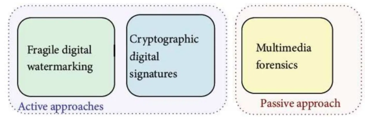
Knowing the original image, it’s easy to understand if the image is acquired with the device that is detected and if the image shows the original captured scene. In practical case, we have not a priori information about the original image, so investigators need to authenticate the image history in a blind way. There are several approaches that can be classified into active and passive

2.2. Image Forensic 7

Figure 2.1: Possible approaches for the assessment of the history and credibility of a digital image.

technologies as shown in Figure 2.1, where for “active” we indicate that for the evaluation of reliability, some information that has been calculated at the source (i.e. in the camera) during the acquisition step, are exploited, while with the “passive” term we indicate that the reliability evaluation is made having only the digital content available.

A major problem of active solutions is that digital cameras are specially equipped with a watermarking chip or a digital signature chip that, exploit-ing a private key hard-wired in the camera itself, authenticates every image the camera takes before storing it on its memory card. To overcome this problem, a new set of methods for authenticating the contents of digital im-ages without using any prior information, defined as passive, have evolved quickly. This technology is defined as multimedia forensic, and the idea is that each phase of the image history (the acquisition process, its storing in a compressed format and any post processing operation), leaves a distinctive trace on the data, like a digital fingerprint. Is therefore possible to identify the source of the digital image or determine if it is authentic or not, looking if the features intrinsically tied to the digital content are present, absent or in-congruous. Multimedia forensics descends from the classical forensic science, which studies the use of scientific method to obtain significant data from physical or digital evidences. The goal of multimedia forensic is to expose the traces left in the multimedia content in each step of its life, exploiting ex-isting knowledge on digital image and in multimedia security research. Here we give some examples on how multimedia forensics works:

2.2.1

Photo-Response Non-Uniformity (PRNU)

Photo-response non-uniformity is an intrinsic property of all digital imaging sensors, due to slight variation among individual pixels in their ability to convert photons to electrons. Pixel are made of silicon and capture light by converting photons into electrons, using the photoelectric effect. We use a matrix K, that has the same dimensions as the sensor, to capture the differences among pixel. By illuminating the imaging sensor with ideally uniform light intensity Y, without noise sources, the sensor would register a noise-like signal Y + YK. The term Y K is usually referred to as the pixel-to-pixel non-uniformity or PRNU. The matrix K is responsible for the major part of what we call the camera fingerprint, that can be estimated experimentally by taking many images of a uniformly illuminated surface, and averaging the images to isolate the systematic component of all the images. YK is the PRNU term, and it’s only weakly present in dark areas, where Y ≈ 0 or in completely saturated areas of an image, that produce a constant signal and do not carry any traces of PRNU.

The factor K is very useful, and its responsible for a unique sensor fingerprint; has the properties of dimensionality (the fingerprint is stochastic in nature and has a large information content, which makes it unique to each sensor), universality (all imaging sensors exhibit PRNU), generality (the fingerprint is present in every picture, with the exception of completely dark images), stability (is stable in time and under wide range of environmental conditions, like temperature or humidity) and robustness (it survives lossy compression, filtering, and many other typical processing).

The fingerprint can be used for many forensic tasks; for example, by testing the presence of a specific fingerprint in the image we can prove that a certain camera took a given image, or prove that two images comes from the same camera. We can also see if the image is natural or modified: by testing the absence of the fingerprint in individual image regions, we can find areas of the image that has been replaced. By detecting the strength or form of the fingerprint, we can reconstruct some of the processing history. We can use the spectral and spatial characteristics of the fingerprint to identify the camera model or distinguish between a scan and a digital camera image. For more details, refer to Fridrich [5]

2.2. Image Forensic 9

2.2.2

Camera Model Identification

A problem that we aim to solve is to detect the camera model (and the brand of this camera) used to shoot a picture to solve some forensic problems, like copyright infringement to ownership attribution. The forensic community has developed a set of camera model identification algorithms that exploit characteristic traces left on acquired images, by the processing pipelines spe-cific of each camera model.

The idea is that each camera model implements a series of characteristic complex operations at acquisition time, from focusing light rays through lenses, to interpolation of color channels by proprietary demosaicing filters, to brightness adjustment and others. These are non-invertible operations, and for this reason they introduce some unique artifacts on the final image, that are footprints that help to detect the used camera model. The problem of camera model identification consists in detecting the model L (within a set of known camera models) used to shoot the image I. A possible solution for this problem is to use a convolutional neural networks (CNN). We will give an overview on CNN in Section 3.2.2.

For further details look at Bondi et al. [6].

2.2.3

Double JPEG compression

When we save an image, usually it is saved in JPEG format. For this reason, when we manipulate the content, a JPEG re-compression happen. Often, manipulation takes place on small parts of the image, and therefore, being able to detect DJPEG on small image patches is important for localization of manipulated regions in image forgery detection problems.

JPEG is an image transform coding technique based on block-wise Discrete Cosine Transform (DCT). An image is split into 8×8 non-overlapping blocks, then each block is DCT transformed and quantized, and at the end the en-tropy is coded and packed into the bitstream. Quantization cause the loss of informations, and is driven by pre-defined quantization tables scaled by a quality factor (QF). If QF is low, a strong quantization occurs, and the final decompressed image has lower quality. We have a double compression when an image compressed with a quality factor QF1 is first decompressed, and then compressed again with quality factor QF2. If between the two compres-sion no operations are made, we speak of A-DJPEG comprescompres-sion, since 8 × 8 JPEG blocks of the first and second compressions are perfectly aligned. If

the second compression 8 × 8 grid is shifted with respect to the previous one, we have a NA-DJPEG compression (e.g. cropping or cut and paste operation between the two compressions). We want to build a detector which is able to classify between single and double compressed images: if H0 correspond

to the hypothesis of single compressed image, and H1 to the hypothesis of

double compressed image, given a B × B pixel image I, we want to detect if H0 or H1 is verified. We consider the following case: only A-DJPEG, only

NA-DJPEG or both A-DJPEG and NA-DJPEG. We need to use different approaches because aligned and non-aligned DJPEG compression leave dif-ferent footprints and then cannot be detected in the same way.

Chapter 3

Problem Formulation

In this Chapter we define the goal of our work and the characteristics of the studied problem, providing a general idea on how we can find the solution. Then, we describe the dataset on which our analysis are made, and at the end we introduce the main background concepts and state-of-the art algorithms.

3.1

Motivation and problem statement

It’s always easier to modify the content of an image, thanks to the many im-age processing software, both for personal computer and smartphones, and for this reason the forensic community has developed a series of techniques to asses image authenticity. Another important problem to be solve from the forensic community is the copyright infringement to ownership attribution. We can detect if an image has been edited because all non-invertible opera-tions applied to a picture leave peculiar footprints, which can be detected to expose forgeries.

Given an image, we want to be able to detect if there are any modified areas, and where they are located.

3.1.1

The dataset

The dataset that we have is composed of a total of 93 images with different dimensions. Each image is divided into N patches, that are made by 64 × 64 pixel. In Table 3.1 we have the number of images that have a certain number of patches, where N is the total number of patches present in the image and the second row tell us how many images have dimension N . We can see that

N 408 850 1230 1380 1764 1850 2301 2745 2852 3690

images 17 21 14 13 3 4 5 7 7 2

Table 3.1: Number of images and dimension

Figure 3.1: Real image and suddivision of the two groups: in blue the original image and in red the modified area

we have a majority of images with small dimension.

A single patch is characterized by the coordinates (y, x), a variable gt that is equal to 0 if the patch belong to the original image, and is equal to 1 if the patch belong to the modified area, and a vector of 419 elements of features f, that represent the characteristics of the patches. The feature vector is extracted from each patch through a slightly modified version of the Convolutional Neural Network presented in [6]. In Fig. 3.1 we have an example of an image, and the true classification. The blue part is the original image, and the red part is the tampered area. In this case we can see that there are two areas that are modified, one is the sky and the other is the crocodile.

3.2

State of the Art

In this section an overview of the literature methods on image tampering detection and localization, and on Convolutional Neural Networks for camera model identification is given.

3.2. State of the Art 13

3.2.1

Image tampering detection and localization

ADQ1 Aligned Double Quantization detection, developed by Lin et al. [8] aims to discover the absence of double JPEG compression traces in tampered 8 × 8 image blocks. Generate for each block the posterior probabili-ties to being possibly tampered, through voting among discrete cosine transform (DCT) coefficients histograms collected for all blocks in the image.

BLK Due to its nature, JPEG compression introduces 8 × 8 periodic arti-facts on images that can be highlighted thanks to Block Artifact Grids (BAG) technique from Li, Yuan, and Yu [9]. We can find traces of image cropping (grid misalignment), painted regions and copy-move positions by detecting disturbances in the BAG.

CFA1 At aquisition time, color images undergo Color Filter Array (CFA) interpolation due to the nature of aquisition process. Ferrara et al. [10] build a tampering localization system detecting anomalies in the statistics of CFA interpolation patterns. A mixture of Gaussian distri-butions is estimated from all the 2 × 2 blocks of the image, resulting in a fine-grained tamper probability map.

CFA2 Dirik and Memon [11] show, by estimating CFA patterns within four common Bayer patterns, that if none of the candidate patterns fits sufficiently better than the other in a neighborhood, then, it’s like tampering occurred. In fact, weak traces of interpolation left by the de-mosaicking algorithm are hidden by typical splicing operations like re-sizing and rotations.

DCT In Ye, Sun, and Chang [12] are detected inconsistencies in JPEG DCT coefficients histograms by first estimating the quantization matrix from trusted image blocks, then evaluating suspicious areas with a blocking artifact measure (BAM).

ELA Error Level Analysis, developed by Krawetz [13], aims to detect parts of the image that have undergone fewer JPEG compression than the rest of the image. It works by re-saving the image at a known error rate and then computing the difference between the original and the re-compressed image. Local minimums in image difference indicate original regions, and local maximums indicate that a tampering occurs. GHO JPEG Ghosts detection by Farid [14] is an effective technique to identify parts of the image that were previously compressed with smaller quality factors. The method is based on finding local minimum in the sum of squared differences between the image under analysis and its re-compressed version with varying quality factors.

NOI1 It’s a tampering detector build by Mahdian and Saic [15] upon the hy-pothesis that usually Gaussian noise is added to tampered regions, with the goal of deceiving classical image tampering detection algorithms. A segmentation method based on homogeneous noise levels is used to provide an estimate of the tampered regions within an image, modeling the local image noise variance trough wavelet filtering.

NOI4 Fontani et al. [16] presented a statistical framework aimed at fusing several sources of information about image tampering. Information provided by different forensic tools yields to a global judgement about the authenticity of an image. Outcomes from several JPEG-based al-gorithms are modeled and fused using Dempster-Shafer Theory of Evi-dence, being capable of handling uncertain answers and lack of knowl-edge about prior probabilities.

3.2.2

CNN for Camera Model Identification

Convolutional Neural Networks are complex nonlinear interconnection of neurons inspired by biology of human vision system. The use of CNNs in forensics is recent. Inspired by results obtained by Bondi et al. [17], we take the proposed CNN as a feature extractor for each patch of the input image. The structure of a CNN is divided into several blocks, called layers. Each layer Li takes as input either an Hi× Wi× Pi feature map or a feature vector

of size Pi and produces as output either an Hi+1× Wi+1× Pi+1 feature map

or a feature vector of size Pi+1.

3.2. State of the Art 15

• Convolutional layer Performs convolution, with stride Sh and Sw

along the first two axes, between input feature maps and a set of Pi+1

filters with size Kh× Kw× Pi. Output feature maps have size

Hi+1= jH_i − K_h+ 1 Sh k , Wi+1 = jW_i− K_w+ 1 Sw k , and Pi+1.

• Max-pooling layer Perform maximum element extraction, with stride Sh and Sw along first two axes, from a neighborhood of size Kh× Kw

over each 2D slice of input feature map. Output feature maps have size Hi+1= lH_i − K_h+ 1 Sh m , Wi+1 = lW_i− K_w+ 1 Sw m , and Pi+1= Pi.

• Fully-connected layer Performs dot multiplication between input feature vector and weights matrix with Pi+1rows and Pi columns.

Out-put feature vector has Pi+1 elements.

• ReLU layer Performs element-wise non linear activation. Given a sin-gle neuron x, it is transformed in a sinsin-gle neuron y with y = max(0, x). • Softmax layer Turns an input feature vector to a vector with the same number of elements summing to 1. Given an input vector x with Pi neurons, xj ∈ [1, Pi], each input neuron produces a corresponding

output neuron y_j = e

xj

Pk=Pi

k=1 exk

.

The network proposed by Bondi et al. [17] is an 11 layer CNN structured as follows:

• An RGB color input patch of size 64 × 64 is fed as input to the first Convolutional layer with kernel size 4×4×3 producing 32 feature maps as output. Filtering is applide with stride 1.

• The resulting 63 × 63 × 32 feature maps are aggregated with a Max-Pooling layer kernel size 2 × 2 applied with stride 2, producing 32 × 32 × 32 feature maps.

• A second Convolutional layer with 48 filters of size 5 × 5 × 32 applied with stride 1 generates 28 × 28 × 48 feature maps.

• a Max-Pooling layer with kernel size 2×2 appied with stride 2 produces a 14 × 14 × 48 feature maps.

• A third Convolutional layer with 64 filters of size 5 × 5 × 48 applied with stride 1 generates 10 × 10 × 64 feature map.

• A Max-Pooling layer with kernel size 2×2 applied with stride 2 produces a 5 × 5 × 64 feature map.

• A fourth Convolutional layer with 128 filters of size 5 × 5 × 64 applied with stride 1 generates a vector of 128 elements.

• A fully connected layer with 128 output neurons followed by a ReLU layer produces the 128 element feature vector.

• A last fully connected layer with Ncams output neurons followed by a

Softmax layer acts as logistic regression classifier during CNN training phase. Ncams is the number of camera model used at CNN training

stage.

A shown in Bondi et al. [17], the trained CNN is able to extract meaningful information about camera models even from images belonging to cameras never used for training the network. This property enables exposing forgeries operated also with unknown camera models.

3.2.3

Splicebuster

Splicebuster is a feature-based algorithm to detect image splicing, proposed by Cozzolino, Poggi, and Verdoliva [18]. Splicing is the insertion of material taken from a different source, without any prior information on the host camera, on the splicing, or on their processing history.

The problem of methods based on machine learning and feature modeling, is that they need a large training set.

The approach used to localize possible forgeries in the image is based on three major steps:

• defining an expressive feature that captures the traces left locally by in-camera processing;

• based on a suitable training set, compute synthetic feature parameters (mean vector and covariance matrix) for the class of images under test;

3.2. State of the Art 17

• use these statistics to discover where the features computed locally depart from the model, pointing to some possible image manipulation. We have a single image with no prior information, so we must localize the forgery and estimate the parameters of interest at the same time. We con-sider the supervised case, in which the user has to select a tentative training set to learn the model parameters, and the unsupervised case, where simul-taneous parameter estimation and image segmentation are done jointly by means of the expectation-maximization (EM) algorithm.

Co-occurrence based local feature Feature extraction is base on three main steps:

1. computation of residuals through high-pass filtering: we use a linear high-pass filter of the third order, that is defined as rij = xi,j−1 −

3xi,j + 3xi,j+1 − xi,j+2, where x and r are origin and residual images,

and i, j indicate spatial coordinates. This type of filter assure us a good performance for both forgery detection and camera identification. 2. quantization of the residuals: we perform quantization and truncation

as ˆrij = truncT(round(rij/q))1, where q is the quantization step and T

the truncation value.

3. computation of a histogram of co-occurrences, on four pixels in a row, that is: C(k0, k1, k2, k3) = P_i,jI(ˆri,j = k0, ˆri+1,j = k1, ˆri+2,j = k2, ˆri+3,j =

k3), where I(A) is the indicator function of event A, equal to 1 if A

holds and equal to 0 otherwise.

Supervised scenario In this case, the user has an active role in the process, by selecting a bounding box that will be subject to the analysis (including the possible forgery); the rest of the image is used as training set. The N blocks taken from the training area are used to estimate mean and covariance of the feature vector h0, extracted from each block of the test area, as follow: µ = 1 N N X n=1 hn

1_{Remember that truncation is defined in the following way: given a number x ∈R} +

to be truncated and n ∈N0 the number of elements to be kept behind the decimal point,

the truncated value of x is: truncn(x) =

b10n_{· xc}

Σ = 1 N N X n=1 (hn− µ)(hn− µ)T

Then the Mahalanobis distance with respect to the reference feature µ is computed:

D(h0, µ; Σ) = (h0− µ)T_Σ−1

(h0− µ)

The greater the distance, the more the blocks deviate from the model. Then, the user provide an output map, where to each block is given a color associ-ated with the computed distance.

Unsupervised scenario In this case, after the feature extraction phase, we use an automatic algorithm to jointly compute the model parameters and the two-class image segmentation. As input, we need the mixture model of the data (number of classes, their probabilities, and the probability model of each class). Consider two cases for the class models:

1. both the original area (hypothesis H0) and the tampered area

(hypoth-esis H1) are modeled as multivariate Gaussian:

p(h) = π0N(h|µ0, Σ0) + π1N(h|µ1, Σ1);

2. the genuine area of the image is modeled as Gaussian, while the tam-pered area is modeled as Uniform over the feature domain Ω,

p(h) = π0N(h|µ0, Σ) + π1α1I(Ω);

The Gaussian model is a simplification, and is conceived for the case when the edited area is relatively large with respect to the whole image.

However, when the modified region is very small the intra-class variabil-ity may become dominant with respect to inter-class differences, leading to wrong results. Therefore, we consider Gaussian-Uniform model, which can be expected to deal better with these situations, and in fact has been often considered to account for the presence of outliers.

Chapter 4

Proposed solutions

In this Chapter we will describe the Bagging-Voronoi algorithm, showing its structure, the theoretical details and the properties.

In Section 4.1 the Bagging-Voronoi algorithm for clustering spatially depen-dent data is introduced and described. In section 4.2 the algorithm is ex-plained in detail. In Section 4.3 are shown the changes to be applied to the algorithm in presence of data whose geometry is known and finally, in Section 4.4 we propose a set of improvements.

4.1

Geometry-aware clustering algorithm

Let call site x each patch of our image, that are the elements that we want to group using the clustering algorithm, and let be the latent label l ∈ {1, . . . , L} be the group assigned to the site x. We call the whole image S0.

The problem consists in associating to each site x ∈ S0 a latent label

l ∈ {1, ..., L}, such that sites that present similar characteristics are labeled the same. We aim to identify different homogeneous macro-areas. Using the standard clustering techniques, such as K-means, do not properly account for spatial dependence, and so, when we assign a site to a cluster, informa-tion carried by neighboring sites are not considered. For a given number K of clusters, the proposed spatial clustering procedure generates and ana-lyzes bootstrap samples in three basic steps: generation of a spatial random Voronoi tessellation with dimension n, identification of a local representative for each of the n tessellation, considering all the elements contained in the tessellation and clustering of the local representatives.

Lets describe the Bagging-Voronoi algorithm, following the pseudo-code scheme in Algorithm 1.

Algorithm: Bagging-Voronoi classifier.

Data: A matrix that contain, for each patch, the coordinate and the characteristics

input : B,n,θ,K

output: A final classification map Bootstrap:

for b ← 1 to B do

step 1. randomly generate a set of nuclei φb

n= {Z1b, ..., Znb}

among the sites in S0: for i = 1, ..., n, Zib iid

∼ U (S0), where U is

the uniform distribution on the lattice. Obtain a random

Voronoi tessellation of S0, {V (Zib|φbn)}ni=1, by assigning each site

x ∈ S0 to the nearest nucleus Zib, according to the euclidean

distance;

step 2. for i = 1, ..., n, compute the local representative gb i, by

summarizing information carried by the data associated to sites belonging to the i-th element of the tessellation V (Zb

i|φbn);

step 3. perform clustering on the local representatives {gb

1, . . . , gnb} using an unsupervised method;

end

Aggregation

step 1. perform cluster matching: for k = 1, ..., K, and b = 1, ..., B; indicate with C_kb the set of x ∈ S0 whose label is equal to k at the

b-th replicate, and match the cluster labels across bootstrap replicates, to ensure identifiability;

step 2. assign each x to the most frequent label; step 3. compute spatial entropy ηK

x for each site x ∈ S0;

Algorithm 1: Pseudo-code of the Bagging-Voronoi classifiers algo-rithm

Suppose a latent field of labels Λ0 : S0 → {1, ..., L} is defined on the

4.1. Geometry-aware clustering algorithm 21

where S0 is a subset of Rp. In our case S0 is a subset of R2, and represents

the whole image. A single image contains N different patches, that are made by 64 × 64 pixels. So each site x corresponds to a single patch.

For each site x we have some information, given in a vector of features f ∈ [0, 1], that sum up to 1. The algorithm perform first a bootstrap sam-pling phase, that is divided in three steps, and then an aggregation phase, where at each iteration of the algorithm a single weak classifier is found, which exploits a specific structure of spatial dependence. After B different runs of the algorithm, bagging together all single classifiers, we can obtain a more accurate global classifier.

In step 1 of the bootstrap sampling part, we generate a random Voronoi tessellation, to capture potential spatial dependence. In step 2 we identify a local representative for each tessellation, summing up local information from all the elements contained in the block: we expect that neighboring site are drawn from the same distribution. Then the local representatives are grouped in K clusters according to a suitable unsupervised method (we will use K-means clustering and Partitioning Around Medoids), and all the sites x contained in the tessellation are labeled the same. We have to perform cluster matching to ensure coherence of cluster assignments across replicates. After having done all the iterations, each site x is assigned to the most frequent label. The result depends on the choice of some parameters: the number of iterations B (the higher is B less random are the results), the number of tessellation n (the higher is n, the less the spatial dependence is taken into account), the variance of the Gaussian θ (that takes into account the spatial dependence range) and the number of clusters K.

In order to select the most appropriate value of n, the number of cells pro-duced by the Voronoi tessellation, if we don’t have any other information on the correct label of the data, we can try to use the spatial entropy crite-rion, as suggested by Secchi, Vantini, and Vitelli [1]. Consider the frequency distribution of assignment πx = (πx1, . . . , πKx) of each site x ∈ S0 to each of

the K clusters. The entropy associated to the final classification in the site x ∈ S0 is obtained as η_xK = − K X k=1 πk_x· log(πk x) (4.1)

which assumes minimum value 0 when there is an r such that π_xr = 1 while πk_x= 0 ∀k 6= r, with k, r ∈ {1, . . . , K}, and a maximum value of log(K) when πk

following idea: the more the frequency distribution πxis concentrated on one

particular label, the more the classification is precise and stable along repli-cates. A global evaluation index can be computed as the average normalized entropy ηK = P x∈S0η K x log(K) · |S0| (4.2) including the contribution to the final classification quality of all sites in S0.

For comparison over different choices of K, the quantity ηK

x in Eq. (4.2) has

been normalized by the factor log(K). We expect the value of ηK _{to be low}

if n is properly chosen in accordance to the (unknown) spatial dependence in the latent field of labels: for an optimal choice of n, few elements of the Voronoi tessellation will cross the borders among regions associated to different labels in the latent field, and high values of the entropy will be very localized along these borders. The entropy criterion generally leads to a choice for K more parsimonious than necessary.

4.2

Details on the Bagging-Voronoi algorithm

Now we will see each step of the Bagging-Voronoi algorithm.

4.2.1

Step 1: Voronoi tessellation

We need to unequivocally define a random tessellation, so we have to select a set of points in S0, where S0 ⊂ R2, as nuclei for the Voronoi tessellation.

Let Φn = {Z1, · · · , Zn} be a set of n points in S0 sampled from a uniform

distribution U(S); these points will be the nuclei of the Voronoi tessellation. For each Zi ∈ Φn define the polyhedron

V (Zi|Φn) = {x ∈ S0 : d(x, Zi) ≤ d(x, Zj), ∀Zj ∈ Φn, i 6= j} (4.3)

to be the Voronoi cell with nucleus Zi for the Voronoi tessellation induced

by Φn, i.e. the set of x ∈ S0 which distance d(·, ·) from Zi is smaller than

each other nucleus Zj 6= Zi. The collection {V (Zi|Φn)}ni=1 forms a Voronoi

tessellation of S0. The final tessellation will depend on the choice of the

metric; for our analysis we have taken d(·, ·) as the euclidean distance. For more details on the properties of the Voronoi tessellation look at Penrose [19].

4.2. Details on the Bagging-Voronoi algorithm 23

The most interesting property for our purposes is the coverage property. Consider the collection of Lebesgue measurable sets {Al}Ll=1, Al ∈ S0 for

l = 1, . . . , L, and let Vi = V (Zi|Φn); moreover, let

An_l = [

Zi∈Al Vi ,

be an approximation of Al given by the Voronoi cells whose nuclei belong

to Al. The coverage property states that, for l = 1, . . . , L, the set Anl is a

consistent estimator of the unknown set Al in the sense that

µ(An_l∆Al) a.s.

→ 0, n → ∞, (4.4)

where ∆ denotes the symmetric difference between two sets and µ is the Lebesgue measure.

This property represents a strong law of large numbers in the context of Voronoi tessellations. The Eq. (4.4) is essential for the validity of our algo-rithm, since it states that, when the tessellation becomes less and less coarse, subsets of the domain S0 associated to the same label are well approximated

by suitable sets of Voronoi elements. Indeed, we define the collection of sets {Al}Ll=1 by setting, for l = 1, . . . , L,

Al= {x ∈ S0 : Λ(x) = l},

4.2.2

Step 2: local representatives

For each element Vi of the Voronoi tessellation, we sum up the information

contained in the sub-sample {fx}x∈S0, where f is a vector containing some information for x, by calculating a local representative trough a method that exploits spatial dependence of neighboring data.

For i = 1, . . . , n, the local representative gi of the sub sample {fx}x∈Vi is computed as a weighted mean with a Gaussian kernel:

gi(t) = P x∈Viw i xfx(t) P x∈Viw i x , (4.5) where wi

x is a Gaussian weight centered in Zi and decreasing with respect

to d(x, Zi). Intuitively, we assume that spatial dependence between two

sites decreases when the distance between them increases. We take as kernel covariance the matrix σ2_{Θ, where Θ is a bi-dimensional matrix that has value}

Θij = 0, if i 6= j and Θij = θ if i = j, and where σ = dmax/dmin, with dmax

and dmin the maximum and minimum distance between two nuclei of the

Voronoi tessellation, respectively.

The choice of n, that is the number of tessellation to be generated, has an influence on the algorithm behavior. The optimal choice of n is the one that finds a good compromise between variance and bias:

• as n decreases, noise is reduced in the computation of the local rep-resentatives in Eq. (4.5), since the sub-samples are, in average, larger (minimal variance). However, at the same time the associated Voronoi tessellation follows less accurately the boundaries in the true latent field of labels, thus including different mixture components in the com-putation of local representatives (maximal bias). The limiting case is n ≡ 1, when all sites in the finite lattice belong to the same Voronoi element, and are all used to compute a single representative.

• as n increases, the resulting Voronoi tessellation approximates more accurately the boundaries of the latent field of labels (minimal bias), but at the same time the variability reduction due to spatial smoothing is smaller (maximal variance). The limiting case is n ≡ |S0|, when all

sites in the finite lattice are nuclei, and thus no spatial smoothing is performed.

The optimal value of n determined by this trade-off depends both on the strength of spatial dependence, and on the mixture components of the dis-tribution generating the data.

4.2.3

Step 3: Clustering and aggregation

Once we have obtained the local representatives, we need to search for clus-ters over them and obtain a classification map. For our problem we have decided to use the K-means algorithm.

At each iteration b of the bootstrap phase of the algorithm, a label ˆlb

1, . . . , ˆlbn

is assigned for each local representative, where ˆlb

i ∈ {1, 2, . . . , K} corresponds

to the cluster assignment of the representative gb

i to one of the K clusters,

for i = 1, . . . , n. This assignment will be the same for all the sites x ∈ Vb i .

At each iteration a different classification map is generated, and the problem is that there can be inconsistency between two different iterations. Let C_kb be the set of site x ∈ S0 whose label is equal to k at the b-th replicate. To

4.3. Algorithm knowing the geometry of the data 25

obtain the final classification map, we consider the frequency distribution of assignment of each site to each of the K clusters along the B replicates. To compute this frequency distribution we need to assume that cluster labels {Cb

1, . . . , CKb } are coherent with {C11, . . . , CK1}, for all b ≥ 2 and b ≤ B. We

can do this performing cluster matching between the first replicate and the current one. The algorithm searches the label permutation that minimizes the total sum of the off-diagonal frequencies in the contingency table describ-ing the joint distribution of sites along the first classifications and the current one. It’s possible to use also other cluster matching procedure.

4.3

Algorithm knowing the geometry of the

data

In this section are shown the changes that we have to do in our algorithm when we know the property of our data. In our case we know that the features are similar in accordance to the cosine similarity distance, that is, for two vectors A and B:

similarity = cos(θ) = A · B

||A||||B||. (4.6)

For our image, at each site x is associated a vector f of features, that contain some characteristics for the site; if we consider f1, . . . , fn be the vectors that

contain, for each feature the value associated to all the sites x ∈ S0, then

more are fi and fj similar and more the value of similarity will be high.

The idea is to compute the similarity distance on the local representatives, before clustering. Instead using k-means, we use partitioning around medoid, so we can take better into account the description of our data; since the Eq. (4.6) give us a similarity matrix, which elements are ∈ [−1, 1], first we standardize the result to be in [0, 1], and then we compute the dissimilarity matrix doing 1 − similarity, as shown in Eq. (2.2)

Let consider the local representative gb

i, for i = 1, . . . , n at the iteration b.

The matrix of similarity is a symmetric matrix of dimension n × n, where n is the number of Voronoi tessellations that we build. We construct the dissimilarity matrix in the following way:

R[i, j] = 1 − 1 2 · gb i · gbj ||gb i||||gbj|| + 1 ! . (4.7)

From Eq. (4.7) we can see that more the two local representative would have similar characteristics and more R[i, j] would be close to 0. On the diagonal, all the elements are equal to 0.

4.4

Improvements

In this section we will explain some improvements that we included in our algorithm.

4.4.1

Bagging-Voronoi exploiting more the euclidean

distance

We expect that sites contained in the modified area are all close one to the other, and that there is not a single site that belong to the edited area, if all the neighboring sites belong to the original image. To solve this problem we consider, in addition to the geometry of the data taken into account by the Voronoi tessellation, also the euclidean distance that there is between two sites. So, we will give in input to the pam function a matrix

M = α · R + (1 − α) · D,

where R represent the matrix with the dissimilarity described in Section 4.3, and take into account the geometry of the data, and

D[i, j] =            1 q Zb_i[i, 1] − Zb_i[j, 1])2_{+ (Z}b i[i, 2] − Z b i[j, 2])2 , if i 6= j 1, if i = j

take into account the euclidean distance between the nuclei Z of the i-th and the j-th tessellation, at the b-th iteration. D is, like R, a symmetric matrix with dimension n × n, and take values ∈ (0, 1).

Higher is D[i, j] and smaller is the distance between the nuclei Zi and Zj,

and higher is the probability that the two sites belong to the same group. Since the algorithm require as input a dissimilarity matrix, we have to do D = I − D, where I is a matrix that has values equal to 1 in each element. α is the weight that we give to the geometry of the data and to the euclidean

4.4. Improvements 27

distance: α = 0 means that we are using only the euclidean distance between nuclei, and α = 1 means that we are using only the geometry of the data, and correspond to the case explained in Section 4.3.

4.4.2

Changing the acceptance criterion

Up to now, we decided to assign a site x to the most frequent label. If we consider the local entropy associated to the final classification in each site x, defined in Eq. (4.1), we have that when the site x is almost always classified in the same way, then this value is small, and when at each iteration we assign the site x to a different label, then the value of the local entropy would be very high.

If the Bagging-Voronoi cannot detect the two groups, this means that the most frequent label in the site x is not the correct one, but can be that the entropy in the modified area is very high, because in certain iterations the algorithm classify the related sites in a correct way. It’s reasonable to think that this may happen specially when the tampered area is small or divided in two areas, since in the Voronoi block there will be more sites coming from the original image.

The idea is, instead to assign a site x to the most frequent label, to assign it to the group of the modified area, if the local entropy is greater than a certain value β, and assign it to the group of the original image otherwise.

Chapter 5

Experimental results

In this section the experimental evaluation of our algorithm is provided. First, In Section 5.1, the result of our analysis are shown when the data geometry is not known. In Section 5.2, supposing to know the geometry of the data, the most significant analysis obtained in Section 5.1 are repeated. In Section 5.3 is shown an attempt of improvement carried out by us. In Section 5.4 an interesting study considering the false positive and false negative is made. In Section 5.5 consideration on the optimal number of clusters K is made, and finally, in Section 5.6, a study considering only some images is done.

5.1

Simulation using Bagging-Voronoi

algo-rithm

In this section are shown the results obtained using the Bagging-Voronoi algorithm described in Section 4.1-4.2.

We evaluate our result using the Matthews correlation coefficient (M CC) that is a metric widely used in bioinformatics.

Having defined some metrics in Table 5.1, where Y represent the assigned group and X the original group, we can define the Matthews correlation coefficient as follow:

M CC = T P × T N − F P × F N

p(T P + F N)(T P + F P )(T N + F P )(T N + F N). (5.1) For us, 1 corresponds to the modified area and 0 corresponds to the original area of the image. We decided to use this evaluation metric because it takes

Metric Definition Description

TP P(Y=1,X=1) True Positive (correctly identified) TN P(Y=0, X=0) True Negative (correctly rejected

TPR TP/(TP+FN) True Positive Rate

FN P(Y=0,X=1) False Negative

FP P(Y=1, X=0) False Positive

TNR TN/(FP+TN) True Negative Rate

Table 5.1: Definitions of the elementary metrics used to formulate the evaluation metrics

into account true and false positives and negatives, and it’s a metric that can be used even if the classes are of very different sizes, like may happen in our case.

For the first analysis that we made, we fix the number of clusters K equal to 2.

After a set of preliminary tests, we fix a number of iterations B equal to 31, because further increasing this value did not improve the results. Then, we set intuitively the number of tessellation n = 300 and the variance of the Gaussian distribution θ = 1. Using these values for the parameters, we perform a simulation of all the 93 images contained in our dataset, and we obtain a mean M CC equal to 0.542, that represent our baseline.

5.1.1

Optimal length of the tessellation

The aim of this first test is to search for an optimal number of tessellation to select, inspired by what was done by Volpe [20] . Since in our dataset we have images of different sizes, instead to consider the number of tessellation n to generate we consider the average length of a block l, that is defined as l = N/n, where N is the dimension of the whole image, i.e. the number of patches that we have. Therefore, the optimal number of tessellation will be n = bN/lc.

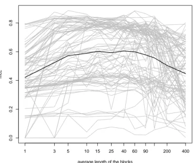
We consider l = {1, 3, 5, 10, 15, 25, 40, 60, 90, 125, 200, 400} and we evaluate, for each length l of each image, the M CC and the average normalized entropy, that from now we will call AN E and that was defined in Eq. 4.2.

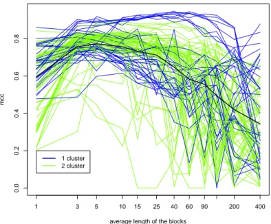
5.1. Simulation using Bagging-Voronoi algorithm 31 0.0 0.2 0.4 0.6 0.8

mcc with respect to the average length of the blocks

average length of the blocks

mcc

1 3 5 10 15 25 40 60 90 200 400

Figure 5.1: MCC value with respect to the average length in a block, considering B=31, K=2 and Gaussian variance equal to 1

average length, as suggested by Secchi, Vantini, and Vitelli [1] and verified by Volpe [20], also when real data are used instead of synthesized ones.. We obtain the result shown in Figure 5.1, where the black lines represent the mean values and the gray lines represents the value obtained for each single image.

Looking at Figure 5.1 we can see that at the beginning the mean value of the M CC is increasing, then it remains approximately constant between l = 5 and l = 60 and then it decreases. This trend justifies the advantages given by using the Bagging-Voronoi algorithm, since for l = 1 (that means that each tessellation contain a single element) we have smaller values than taking larger values of l. Otherwise, if a single tessellation has to many elements (when l increases), when we compute the local representative we are losing too much information, thus, also in this case the results are not so good.

The mean curve present a maximum for l = 15, that correspond to M CC = 0.603, that is greater than the value found in the first simulation done with a generic n = 300. Although the mean curve has an ideally shape, we cannot

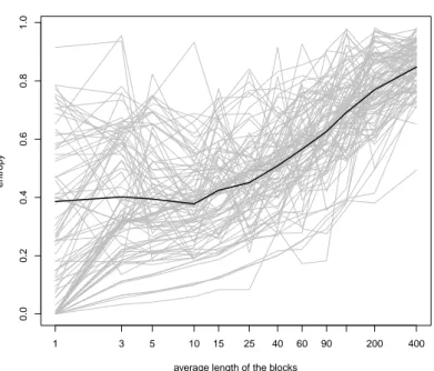
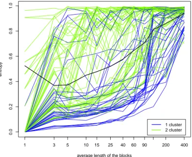
0.0 0.2 0.4 0.6 0.8 1.0

entropy with respect to the average length of the blocks

average length of the blocks

entrop

y

1 3 5 10 15 25 40 60 90 200 400

Figure 5.2: MCC value with respect to the average length in a block, considering B=31, K=2 and Gaussian variance equal to 1

say this for the gray lines, which are the values of the M CC for the single images. In particular, we can see that there are some images for which the algorithm it’s not able to detect the tampered area for all the values of l and other images for which the lines fluctuate. Looking at the images for which we have obtained the best results we notice that the M CC is not much greater than 0.8.

Let analyze now Figure 5.2, that shows the AN E with respect to the average length of a block. We notice that the mean line starts in a flat way, presents a minimum for l = 10 and then increases. For the mean point in l = 1 we have not considered the points with AN E = 0, that are the points clustered, at each iteration, in the same way. When l is large, also the value of the AN E is very high, and this make sense because the local representatives that we build have a lot of variance, and for this reason the result depend a lot of the random initialization of the nuclei; the result is that most of the patches are assigned at one or another group with high uncertainty.

Observing the gray lines, that correspond to the single images, we notice that there are few images for which the AN E value is low, and other images for

5.1. Simulation using Bagging-Voronoi algorithm 33 0 1000 2000 3000 0 100 200 300 400

Optimal length of the blocks vs dimension of the image considering mcc

dimension N of the image

l optimal

Figure 5.3: l optimal vs dimension N of the image, considering B=31, K=2 and Gaussian variance equal to 1

which the AN E value oscillates.

Looking at the two plots it seems that there is a small relation between the goodness of classification and the AN E, since taking the smallest value for the mean AN E, that is l = 10, we have one of the highest value of the M CC (we obtain 0.589 versus 0.603 obtained with l = 15). The problem is that this reasoning is true only looking at the mean line. For the single images it is more complicated to search for the optimal value, and it’s not always true that taking the minimum value from the AN E and selecting the corresponding l, give us an high M CC.

5.1.2

Optimal length of the tessellation with respect

to the dimension of the image

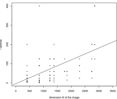
As we have seen, our dataset contain images that have different dimension. A question we asked ourselves is if there is a relation between the optimal average length of a block and the dimension of the image. We proceed in the following way: first we calculate all the values of M CC for all the average

0 500 1000 1500 2000 2500 3000 3500 0 100 200 300 400

Optimal length of the blocks vs dimension of the image considering mcc

dimension N of the image

l optimal

Figure 5.4: l optimal vs dimension N of the image, considering B=31, K=2 and Gaussian variance equal to 1, with the regression line

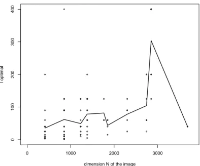
lengths of the block l = {1, 3, 5, 10, 15, 25, 40, 60, 90, 125, 200, 400}; then, for each image, we have searched the highest value obtained in terms of M CC, and we have saved the corresponding optimal average length l∗ of the block. The result is the plot in Figure 5.3, where the black line represents the mean optimal length of the tessellation for each N . We can notice that for the same dimension N of the image, we have very different average optimal length of the tessellation. This happen because even if two images have the same dimension N , their content and the dimension of the edited area may be very different, and so, for some images K-means works better with small l while for the other K-means work better with a larger l.

If we don’t consider the points for N = 3680, that are only 2, it seems that there is a little increasing of l∗, when N increases. We can see that there are some outliers like the two points which result is l∗ = 400.

The idea was to search for a regression line between, but looking at Figure 5.3 it seems that there is not a linear relation between the optimal average length of the tessellation and the size of the image. To confirm our suppositions, we build it, and the best regression model that we get, after trying also to not

5.1. Simulation using Bagging-Voronoi algorithm 35

consider the outliers, is the one in Figure 5.4, where we don’t have considered the points in N = 3680. For this model we obtained a R2 = 0.2697 that is very low: this means that only 26.97% of all the data are well explained by this model. This regression line correspond to the following equation:

l∗ = −3.80555 + 0.06182 · N (5.2)

We also tried to do this analysis considering, instead of the highest value of the M CC for each image, the first 3 highest value of the M CC, if they where sufficiently good, because for some images the Bagging-Voronoi algorithm gives good result for more than one value of l. But also in this case there is not a relation between the optimal value of l and the dimension N of an image.

Since this result is not significant, we will no longer consider this type of analysis, and we will set l = 15 for all the following experiments.

5.1.3

Gaussian variance choice

In this section we will do some considerations about the variance of the Gaussian, that is another parameter that may change our results. Recall that the local representatives gi, for i = 1, . . . , n of the sub-sample {fx}x∈Vi were computed as a weighted mean with a Gaussian kernel (see Eq. 4.5). Taking a smaller value of the variance, means that we are shrinking the Gaussian kernel, and that the values near the nuclei (in our case the Gaussian distribution is centered in the nuclei) are considerate much more than distant points. Otherwise, taking a bigger value of the variance, means that we are spreading the Gaussian kernel, and there is less difference in the weight of the values of fx between near and far points from the nuclei.

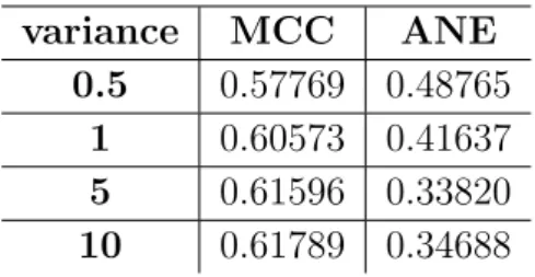
We consider B = 31, l = 15 (that was the best value that we obtained in Section 5.1.1), K = 2, and we computed, for all the 93 images and for the Gaussian variance θ = (0.5, 1, 5, 10), the mean value of the M CC and of the AN E. We obtained the results shown in Table. 5.2

Looking at this results, we can see that it seems that an higher variance give us better results. This happen because we have, on average, l = 15 elements par tessellation, and a too small variance cannot be able to consider appropriately all the elements of the block.

An interesting thing is that it seems to be a relation between the optimal variance value and the AN E: in fact, except for θ = 10, where the increment

variance MCC ANE

0.5 0.57769 0.48765

1 0.60573 0.41637

5 0.61596 0.33820

10 0.61789 0.34688

Table 5.2: Value of MCC and ANE when the variance of the Gaussian varies

of the M CC with respect to θ = 5 is very low, higher is the M CC and lower is the AN E. So, if we have a set of images without any prior information, a good way to select the optimal value of the Gaussian variance is taking the value that correspond to the lowest AN E, since when the value of the M CC increase a bit, the AN E decreases much more.

5.1.4

Final consideration

The significant result that we obtained from this analysis are the following: • looking at the minimum mean value of the AN E, we can select the

optimal value of the length of the tessellation;

• a good average length of the tessellation is l∗ _{∈ (5, 90);}

• there is no relation between the number of tessellation to take and the dimension of the image;

• the variance of the Gaussian kernel may influence the results, and can be selected by taking the minimum value of the AN E;

A final consideration is that deal with real data is not easy; our results are fine if we look at all together, but if we consider the single images, the results can be very good or not.

5.2

Simulation knowing the geometry of the

data

In this section we suppose to known the geometry of our data; in our case the data are distributed according to cosine similarity distance. We have to