Application of direct policy search to the management of a multy-reservoir system : a study of the Nile river

(1)

POLITECNICO DI MILANO

School of Civil, Environmental and Land Management Engineering

Master of Science in Environmental and Land Planning Engineering

Application of direct policy search to

the management of multi-reservoir systems:

A study of the Nile River

Supervisor:

PROF. GIORGIO GUARISO

Master Graduation Thesis by:

LORENZO CARELLI

Student Id n. 836943

(2)

(3)

I

To DavidOne

“Beautiful is what we see.

More beautiful is what we know.

Most beautiful, by far, is what we don't.”

(4)

II

ACKNOWLEDGMENTS

First and foremost I would like to express my sincere appreciation to my supervisor, Professor Giorgio Guariso, for his guidance, inspiration, suggestions and criticism. I would like to acknowledge my friend, Matteo Sangiorgio, for his help and support during this study.

Special thanks are due to Dr. Marc Jeuland, who shared the results of his work making this thesis possible.

Tutte le persone con cui sono venuto in contatto meritano di essere ringraziate, in quanto l’incontro con ciascuno di loro mi ha reso ciò che sono.

Un grande riconoscimento va a tutta la mia famiglia per avermi sempre sostenuto e incoraggiato, in particolar modo i miei genitori che mi hanno permesso di seguire le mie inclinazioni.

Sono grato a tutti i miei colleghi, nonché amici, di Ing. Matematica ed Ambientale. Accompagnandomi nel percorso accademico avete arricchito la mia esperienza con la vostra compagnia.

Ringrazio tutti gli amici, che mi hanno aiutato nei momenti difficili così come hanno condiviso con me quelli piacevoli.

Infine rendo omaggio a tutti i docenti che ho avuto nel corso degli anni, la cui influenza è stata fondamentale per la mia formazione.

Un particolare ringraziamento a Giulio e ai suoi preziosi consigli, che sono stati inestimabili.

Ultima, ma certamente non per importanza, Giulia, che mi ha rincuorato e ha sempre avuto fiducia nelle mie capacità.

(5)

III

SOMMARIO

Da un punto di vista teorico, l’applicazione della programmazione dinamica stocastica (SDP) di Bellman permette di trovare la politica di controllo ottimo per la gestione di un sistema naturale. Tuttavia l’applicazione pratica di questo algoritmo non è sempre possibile per via della complessità del sistema, del numero di variabili da considerare e la molteplicità degli obiettivi contrastanti. Questo lavoro propone un approccio alternativo al problema di ottimizzazione utilizzando reti neurali artificiali (ANN) per superare i problemi riscontrati con la SDP. Nello specifico viene descritta la ricerca diretta della politica (Direct Policy Search). I risultati di questa metodologia vengono paragonati con quelli ottenuti tramite la regressione di politiche generate tramite ottimizzazione stocastica implicita (ISO). Particolare importanza viene data all’informazione utilizzata come ingresso alle leggi di controllo e come variano i risultati di conseguenza. Il caso di studio preso in esame è il bacino del Nilo per il quale sono stato identificati due obiettivi: minimizzare il deficit idrico delle coltivazioni e massimizzare l’energia idroelettrica prodotta.

(6)

IV

ABSTRACT

From a theoretical point of view, the application of Bellman stochastic dynamic programming (SDP) allows finding the optimal control (OC) policy of a natural resources management problem. However, its practical application to real problem is not always possible mainly due to the complexity of the model of the system, the number of variables to be taken into account and multiple conflicting objectives. This thesis work proposes an alternative approach to an OC problem using artificial neural networks (ANNs) to overcome SDP issues. In particular, this work describes the direct policy search (DPS) method and compares its results with the regression-based implicit stochastic optimization (ISO) approach. The first method solves the OC problem in a single step, obtaining the efficient parametrization of the operating policy. The regression-based algorithm, on the other hand, looks for the optimal open-loop decisions for many given scenario and uses the obtained dataset to identify the closed-loop policy. Another crucial topic of this work is the importance of information used as input of the control laws and the outcome deriving from a different degree of completeness. The proposed case of study is the Nile River Basin circumscribed to two management objectives: minimization of the irrigation water deficit and maximization of the hydroelectric energy production.

(7)

V

LIST OF FIGURES

Figure 2.1: Example of Pareto frontier………..…5

Figure 2.2: Comparison between a pseudo-random sampling and a quasi-random sampling………..…..8

Figure 2.3: Structure of a neuron………15

Figure 2.4: Example of the structure of a neural network……….16

Figure 3.1: Rainfall regimes over the Nile basin. Base period is from 1961 to 1990………..19

Figure 3.2: The four major tributary basins of the Nile River………..20

Figure 3.3: Schematic representation of the Nile River system……….…21

Figure 4.1: Schematic representation of the proposed procedure………..…29

Figure 4.2: Architecture of the Artificial Neural Network used………..31

Figure 4.3: Schematic representation of the method used to define the initial population of GA………33

Figure 5.1: Pareto frontiers resulting from the linear functions………...34

Figure 5.2: Pareto frontiers resulting from the ANN……….35

Figure 5.3: Comparison between the Pareto frontiers obtained using linear functions and ANN………….…35

Figure 5.4: Optimal non-dominated solutions……….37

Figure 5.5: Boxplots representing the distribution of Jhyd in the different scenarios……….38

Figure 5.6: Boxplots representing the distribution of Jirr in the different scenarios……….38

Figure 5.7: Results of the application of linear decentralized-incomplete policies……….40

Figure 5.8: Results of the application of linear decentralized-complete policies………..40

Figure 5.9: Results of the application of linear centralized-incomplete policies………...…41

Figure 5.10: Results of the application of linear centralized-complete policies……….41

Figure 5.11: Results of the application of ANN decentralized-incomplete policies……….…42

Figure 5.12: Results of the application of ANN decentralized-complete policies………..…42

Figure 5.13: Results of the application of ANN centralized-incomplete policies………...43

Figure 5.14: Results of the application of ANN centralized-complete policies………...43

Figure 5.15: Location of the policies selected for the profile analysis………..45

Figure 5.16: Profile analysis of the ANN CI policy that maximize hydroelectric energy production………….46

Figure 5.17: Profile analysis of the ANN CI policy situated in the maximum curvature point of the Pareto frontier……….47

(10)

VIII

LIST OF TABLES

Table 4.1: Input variables considered for each scenario………...30

Table 5.1: Chromatic codification of the scenarios………36 Table 5.2: Performances resulting from policies that maximize hydroelectric energy production and

agricultural irrigation for each considered scenario……….39

Table 5.3: Synthesis of the performances of the models with respect to hydroelectric energy

production……….44

Table 5.3: Synthesis of the performances of the models with respect to hydroelectric energy

(11)

1

1. INTRODUCTION

A typical problem in natural resources management consists of elaborating and applying a control policy to a multi-reservoir system. This kind of system is rather complex under many points of view, starting from the temporal and geographical scales. Another crucial part is linked to the availability of the natural resource in question, which may be used in different - usually contradictory – ways, thus creating conflict of interests. Hydroelectric energy production, irrigation, water pollution and river navigation are only a few examples of stakeholders with potentially conflicting interests. The solution to this kind of problem, if it exists, can be found only through comparison and cooperation among the stakeholders involved in the project. This work presents a possible approach to a multi-reservoir management problem situated in the Nile river basin. For this case of study, only two stakeholders are considered: irrigation and hydroelectric energy production. First of all the river basin has been simplified using a model that could represent the main components of the river network. The utility of the stakeholders has been evaluated through two indicators: water deficit of the agricultural districts and hydroelectric energy produced. In the end, the different scenarios have been compared using the Pareto frontiers generated in each case.

1.1 PROBLEM STATEMENT AND RESEARCH PROBLEMS

In general, a natural resources optimization problem has to consider both planning and management. The first one refers to all those structural actions that are taken once (e.g. the size of a reservoir, whether or not to build a new hydroelectric power plant). The second one regards the distribution of the resource in time and space. This thesis work only refers to a management problem comparing different methods aimed to obtain a control policy, which optimize the performances of the system. These decisions are taken basing on the information available when the decision is applied. Two main drivers influence the system: decisions taken by the decision maker, through which the system can be controlled, and disturbances. The second ones can be divided into two categories: deterministic ones and random ones (Soncini-Sessa et al., 2007). Deterministic disturbances (wt) are known when the control policy is applied. Random disturbances (εt+1), on the other hand, are unknown until they occur, therefore they introduce uncertainty in the system. The DM has to take management decisions (also called controls) at every temporal step. When random disturbances occur, the most effective

(12)

2

approach is the closed-loop one. In this case, the decision takes into account all the information available when the control policy is applied (Maas et al., 1962). If no deterministic disturbances influence the system, the information needed to apply the control is the state of the system (xt), therefore the management decision is a function of the state of the system. That function is called control law and it has to be defined at every temporal step (mt(·)) (Soncini-Sessa et al., 2007). In absence of disturbances, the optimal control can be obtained using an open-loop policy. It consists of a series of control variables (and not a series of control laws as in the closed-loop approach) estimated in order to optimize the performances of the system through the trajectory of the state of the system that is known deterministically (Soncini-Sessa et al., 2007). Since natural systems are subject to random disturbances such as rainfall, closed-loop policies are to be preferred in order to take into account the deviation of the state caused by disturbances. The problem of finding the optimal open-loop control sequence is a mathematical programming problem since we are searching for some parameters (i.e. the decisions on the releases). Conversely, the design of a closed-loop policy, composed by a sequence of control laws, requires the solution of an optimal control problem (i.e. find the optimal control law in a function space). In order to solve such a problem, the approach that could be adopted can either be functional or parametrical (Soncini-Sessa et al., 2007). The first one does not make any assumption over the structure of the control law, which theoretically consists of an infinite series of couples (xt, ut). The practical solution is to discretize both the system and the control law. On the other hand, using a parametric approach, the form of the control law must be defined a priori. In this case, the optimization variables are a finite set of parameters and thus the problem is changed into a mathematical programming problem. The disadvantage of this approach is that we are not considering anymore the entire function space, but the research is limited to a limited portion of it. The aim is now finding the parametrization (Θt) that identify the best control law that belongs to the subspace previously defined.

1.2 PROPOSED PROCEDURE

The proposed procedure consists of using synthetic samples with the same statistical properties of the historic data series as substitutes for the random disturbances so that the uncertainty is removed from the model. The dataset is used to tune the parameters of a fixed class of functions solving the OC problem. Once the parameters are defined, the resulting function is the policy, which is tested on another data series.

(13)

3

This procedure is applied to the Nile River basin. The model has been simplified to obtain a less complex system, more adapt to the purpose. An important feature of this case of study is that there is no international authority to oversee the main dams in the region. As mentioned earlier, the only stakeholders considered in this work are hydroelectric energy production and agricultural irrigation. The Nile River Basin belongs to different States and each power plant and agricultural district looks after its own interests. For academic purposes, the work is conducted under the hypothesis that all the power plants belong to the same company and all the agricultural districts are part of the same consortium. The same system has been simulated in both situation: the different authorities sharing the information and each one of them working alone. From the comparison between the two scenarios, it is possible to figure out if an international authority may benefit the stakeholders considered.

(14)

4

2. BACKGROUND AND RELATED WORKS

Recent decades have witnessed an unprecedented growth in demand for resources. This is mainly due to the growth in population and the rapid industrialization of emerging economies. For this reason, a more efficient management of the limited natural resources available is crucial.

In recent years, many innovative approaches have been developed to solve optimization problems in order to obtain the optimal control policy. A brief overview of the methodology related to multi-reservoir systems optimization is presented in this chapter.

2.1 SINGLE-OBJECTIVE OPTIMISATION PROBLEM

Optimising a multi-reservoir system management implies formalising the problem in mathematical terms. The first step consists of identifying the objectives, i.e. the quantities to be optimized in order to improve the performance of the system. In a SO (Single-Objective) problem the only objective J has to be optimized (conventionally minimize) with respect to the decision variables composing the vector u. The latter in a management problem are called controls and in a multi-reservoir system are mainly represented by water release or derivation. The optimal controls resulting from the solution of the problem will represent a fundamental support tool for the Decision Maker (DM) to manage efficiently the system. To complete the basic formulation of an optimisation problem, equality constraints f(u) and inequality constraints g(u) need to be specified (2.1).

min

𝑢 𝑱(𝒖) (2.1a)

subject to

𝑓(𝒖) = 0 𝑔(𝒖) ≥ 0 (2.1b)

Constraints express the condition under which the system has to be optimised. Basically, they are composed by the dynamic of the system, the deterministic or random disturbances and any other relation between the variables.

2.2 MULTI-OBJECTIVE OPTIMISATION PROBLEM

Generally, the management of a multi-reservoir system involves several stakeholders and different objectives, which may concern hydropower, irrigation, floods, environmental

(15)

5

quality, etc. for instance. It is therefore essential to extend the single-objective techniques describes along the previous paragraphs to the Multi-Objective (MO) case. The concept of Pareto optimality, or efficiency, enables to deal with this issue without necessarily determine a hierarchy of the various objectives. Being impossible to select a solution that optimise every objective without penalising any other, the set of efficient alternatives is composed by all the solutions for which a certain objective cannot be furtherly optimized without any other objective getting worse. The set of Pareto optimal alternatives is called “Pareto Frontier”, shown in figure (2.1) through a graphical example.

Figure 2.1: Example of Pareto frontier.

The Pareto Frontier can be obtained deriving many parametric SO problems from the original MO problem: this is the strategy of the Weighting Method, the Reference Point Method and the Constraint Method. Otherwise, it is possible to solve directly the MO problem through an Evolutionary Multi Objective (EMO) algorithm, which returns Pareto efficient solutions. Giuliani et al. (2014a) presented an example of EMO application in combination with visual analytics to define Pareto optimal solutions.

Castelletti et al. (2013) proposed a Parametric-Simulation Optimization (PSO) method. With this procedure, it is possible to obtain a set of solutions for the MO problem without deriving them from many SO problems that is computationally very demanding.

Once the analyst determines the Pareto Frontier, one among the efficient alternatives is selected through negotiation or political decision. Multiple criteria are available to support the choice; herein we mention the Utopia Point Method, the Indifference Curve Method and the Maximum Curvature Method.

(16)

6

2.3 DETERMINISTIC PROBLEM

If there are only deterministic disturbances, an open-loop control is adequate to manage the system efficiently. The optimal regulation resulting from the design problem will then consist of a sequence of controls (ut), where each element represent the control variable at a certain time step t of the horizon. The evolution of all the involved variables is deterministic and so, at every time step the condition of the system is exactly known, and so is the optimal control.

Otherwise, in presence of any sources of uncertainty, the model cannot predict the exact dynamic of the system a priori. In this case, for every time t, a control law mt(·) (i.e. a function of the state and other possible information), rather than just a control variable, is needed to take into account of the present conditions of the system. Given that, a functional approach is required to solve the management problem.

2.3.1 MATHEMATICAL PROGRAMMING

In the deterministic case, as previously mentioned, the solution of the operation problem consists of just a sequence of values of the control, which can be obtained by solving a mathematical programming problem. More in detail, if both objectives and constraints of problem (2.1) are linear, i.e. J(u), f(u) and g(u) are linear functions of controls u, we are dealing with a Linear Programming (LP) problem. In this case, some appropriate analytic methods can be used requiring restrained computational time. Among these there are the Simplex Method (Dantzig, 1963), the first and the best known one, the subsequent Ellipsoid Method (Khachiyan, 1979) and Projection Method (Karmarkar, 1984), more efficient especially in the case of large dimension of the controls vector.

Although sometimes the design problem can be turned into a linear problem through some approximations and simplifications, it is quite rare to use a LP problem for the optimisation of a multi-reservoir system management. It is definitely more likely to deal with non-linear relations and thus with a Non-Linear Programming (NLP) problem. This kind of problems are not generally solvable with analytic methods and, with respect to the linear case, presents additional difficulties, due to the possibility of multiple stationary points. Therefore, it is necessary for algorithms to avoid selecting a local minimum instead of the global one, which would not provide the optimal solution. Still, the unicity of the solution is guaranteed even for a NLP problem, in some specific cases. In Convex Programming problems (Rockafellar, 1970) the objective function J(·) is indeed convex,

(17)

7

presenting thus a single stationary point. Moreover, the Quadratic Programming (Wolfe (1959) and Beale (1959)) represents a particular case of Convex Programming problem, where the quadratic objective function is also easier to be differentiate thanks to its analytic properties.

2.3.1.1 ITERATIVE METHODS

For the general case of a NLP problem, multiple classes of iterative algorithms are available. Iterative methods renounce to solve analytically the problem at the cost of finding, most of the time, only a suboptimal solution.

Gradient-based algorithms

A common iterative approach is based on the gradient descent, whereby local minima are identified following the direction of maximum decrease of the objective function. The latter is to be evaluated step-by-step starting from an initial point in the space of the optimization variables. The reached local minimum clearly depends on the starting point, therefore many random initialisations are required in order to explore all local minima and identify the absolute one. Moreover, a proper step-size is needed to prevent the divergence of the algorithm. Yet, the main weakness of these methods is that it requires the differentiability of the objective function, which is needed in order to compute the gradient.

Random search approach

Random search optimization methods do not require particular conditions on the objective and on constraints. They take advantage of the computational power of the modern CPUs rather than following a rigorous logical procedure or exploiting analytical properties, according to a heuristic approach. The most important families of algorithms following the random search approach are the Random optimisation methods and the Evolutionary Algorithms, among which a relevant subclass is represented by the Genetic Algorithms. Maier et al. (2014) provided an exhaustive state-of-the-art review of EAs.

Random sampling algorithms (Matyas, 1965) explore the decision space by generating a huge number of random vectors and evaluate for each the objective function. Different strategies have been experimented in order to cover exhaustively the decision space: one is the pseudo-random approach, illustrated in figure 2.2(a), which provides for extracting

(18)

8

random values of the decision vector from a uniform distribution, but fails to reach a homogeneous coverage for a large dimension of the decision vector. In this case, it can be helpful to adopt a quasi-random strategy, illustrated in figure 2.2(b).

Figure 2.2: Comparison between a 2D pseudo-random sampling (a) and a 2D quasi-random sampling (b).

Methods following the random search approach have the advantages of dealing without difficulty with local minima, they do not risk to diverge and do not require any analytical properties. Still many more simulations are necessary with respect to analytical and gradient-based methods, which however are nowadays possible thanks to the computational power guaranteed by more developed computers, specifically through parallel computing.

Among random search methods, Evolutionary Algorithms (EA) are a family of algorithms whose operating principle is inspired by biological evolution. They can be easily adapted to solve multi-objective problems in order to obtain directly all the efficient solutions according to the concept of Pareto optimality: in this case, we are dealing Evolutionary Multi Objective (EMO) algorithms. Giuliani et al. (2016) and Salazar et al. (2016) both presented practical application of this method.

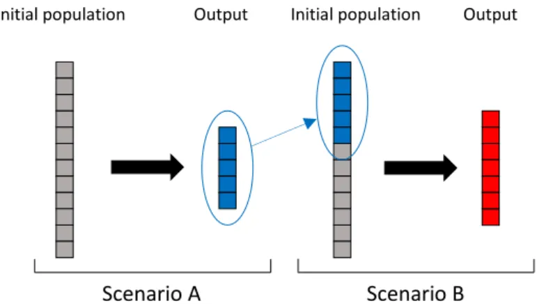
Genetic Algorithms (GA) are a class of evolutionary algorithms used to optimize a function through biological tools such as mutation, crossover and selection (Holland, 1975).

The procedure in this kind of function is inspired by the evolution of the DNA of a species in time, from one generation to another. The starting point of these algorithms is the initial

(19)

9

population. It is a set of possible solutions of the optimisation problem, typically randomly or quasi-randomly generated. Every candidate solution, called individual, belonging to a set called population is evaluated using a fitness function (i.e. the one to be optimized). The best performing individuals are stochastically selected and modified using crossover or introducing random mutations. The resulting individuals represent the next generation and the process repeats itself. There could be many terminating criteria for this iterating procedure. The most common ones are the maximum number of generations or the satisfactory fitness level reached.

2.3.2 DYNAMIC PROGRAMMING

All the previously cited approaches consider the optimal management problem as it was static, but the dynamic of the multi-reservoir system suggests that it can more effectively considered using a dynamic approach. This is the basic principle of the Dynamic Programming (DP) (Bellman, 1957), the most widespread optimisation method used in water resources management (Yakowitz, 1982). The DP provides for quantifying the minimal cost-to-go at each time t through an appropriate function 𝐻_𝑡∗(·), called Bellman function. The choice of the optimal control 𝑢𝑡∗ at each time t is then driven by the need of

minimising at once the present step cost gt and the optimal cost-to-go 𝐻_𝑡+1∗ (2.2) because the decision does not affect only the present step cost 𝑔𝑡(𝑥𝑡, 𝑢𝑡), as clearly evident by the

argument, but indirectly also the optimal cost-to-go 𝐻_𝑡+1∗ _(𝑥 𝑡+1).

𝑢_𝑡∗ = arg min

𝑢𝑡

[𝑔𝑡(𝑥𝑡, 𝑢𝑡) + 𝐻𝑡+1∗ (𝑥𝑡+1) ] (2.2)

The control ut determines indeed in which state xt+1 the system will evolve. The optimal cost-to-go 𝐻𝑡∗ is to be determined step-by-step through the Bellman equation (2.3)

proceeding backwards starting from the last instant of the time horizon h, in which the optimal cost-to-go needs to be initialised with a value H*h(xh), called penalty, representing the cost of leaving the system after the management period in a certain state. Knowing the optimal costs-to-go for every state x of the system at every time step, the sequence of optimal controls is derived easily thought the (2.2).

𝐻_𝑡∗(𝑥_𝑡) = min

𝑢𝑡

[𝑔_𝑡(𝑥_𝑡, 𝑢_𝑡) + 𝐻_𝑡+1∗ _(𝑥

(20)

10

Differently from mathematical programming problems previously illustrated, the DP cannot deal with continuous variables, so states, controls and disturbances need to be discretised to turn the system into a Finite State Automaton (FSA). The discretisation of the system introduces some degree of approximation and the optimal solution of the FSA reveals thus to be actually a sub-optimum with respect to the original system. However, we have to take into account that if the mathematical programming problem is solved through iterative methods, the solution is nonetheless a suboptimum, even if applied to the continuous original system.

The most relevant disadvantage, which severely limits the employment of the DP to minor multi-reservoirs systems, is the so-called “curse of dimensionality”, that is the exponential growth of computational time with the number of states and controls. In addition, an essential condition for the DP is the separability of the constraints and of the objective (J) to be separable. The latter is indeed to be expressed in step costs in order to solve the (2.3). If the objective is not separable, it can be manipulated to be, but at the relevant cost of enlarging the system state, which could exacerbate the problem of dimensionality and computational time. Another issue is the inability of dealing with deterministic disturbances, which should be modelled instead, increasing again the dimension of the state.

2.4 INTRODUCING THE UNCERTAINTY

If the system is affected by any sources of uncertainty, it is necessary to introduce the related disturbance variables, whose value is unknown at the time the decision is taken, and impossible to be deterministically modelled. This uncertainty affects the evolution of the system, so that the state xt at a generic time t is unknown a priori. Rather than a single control ut, for every time t the DM needs a control law mt(·) returning the control value as a function of the state and other possible information available at that time. The operation problem is now an Optimal Control (OC) problem, rather than a MP problem, and the solution is no more a sequence of controls, but a sequence of control laws, called policy. The policy can be obtained as the solution of a design problem extended to the random case, including random disturbance variables, or even by solving many deterministic problems, each including as deterministic disturbance scenario a synthetic realisation of random disturbances (Ahmed et al., 2005).

(21)

11

Introducing stochastic processes in the model is feasible using two different approaches that go under the name of Implicit Stochastic Optimization (ISO) and Explicit Stochastic Optimization (ESO). The first method involves performing deterministic optimization on long data series (historical or stochastically generated), the latter operates directly on stochastic models.

2.4.1 IMPLICIT STOCHASTIC OPTIMIZATION

The application of ISO methods, also referred to as Monte Carlo optimization, consists of three main steps: synthetic dataset generation, optimal releases research for each series and development of the operating rule using the collected data.

The first step provides for the generation of a synthetic long continuous data series or many shorter equally like sequences. Using a dataset of this kind, most stochastic aspects of the problem (such as spatial and temporal correlation) are implicitly included in the model.

Once the inflow series are available, the problem can be solved using deterministic optimization method. For each inflow realization, a different operating policy is found.

At last, all of the policies are examined in order to construct reservoir release rules. Many methods can be applied to achieve this result. A typical approach consists of using multiple regression analysis in order to develop operating rules conditioned on observable information (Labadie, 2004). Another possibility is to use two types of linear equations (Kim & Heo, 2000). Other alternatives to regression analysis are the application of artificial neural networks (Farias et al., 2006; Chandramouli & Deka, 2005) and fuzzy rule-based modelling (Shrestha et al., 1996) to inferring the operating rules.

2.4.2 EXPLITIC STOCHASTIC OPTIMIZATION

ESO is designed to operate directly on probabilistic descriptions of random variables processes than deterministic sequences. In this case, optimization is performed without the presumption of perfect foreknowledge of future events. The application of ESO techniques to multi-reservoir systems is more computationally challenging than ISO (Roefs and Bodin, 1970).

(22)

12

Using ESO methods both inflows and storage levels are regarded as random variables and unregulated inflows are assumed the dominant source of uncertainty that should be represented by appropriate probability distributions.

When random variables are highly correlated, it is possible to create forecasting model in order to generate the data series. This approach is recommended for short-term operation problems, as the forecast errors are the primary source of uncertainty.

2.5 DIRECT POLICY SEARCH

The Dynamic Programming is a powerful tool used in water resources management, but the “curse of dimensionality” prevents its application in presence of a high number of controls and state variables. Considering that each reservoir necessarily implies the introduction of a state variable, this represents a serious limitation for multi-reservoir systems.

In order to deal with this issue, several approaches were introduced. As far as the deterministic problem is concerned, some examples are the Coarse Grid Approximation Technique (Bellman et al., 1962), the State Incremental Dynamic Programming (Larson, 1968) and the Differential Dynamic Programming (Jacobson et al., 1970).

In the random case, the computation costs of the SDP exponentially grow also with the number of disturbance, along with states and controls.

The most effective strategy to overcome the curse dimensionality, necessarily required if we are dealing with a high number of states, controls or disturbances, is abandoning the functional approach for a parametric one (Soncini-Sessa et al., 2007). The class of the function to be determined is fixed except for a limited set of parameters, which are the only variables left to be estimated by solving a mathematical programming problem: it is the basic principle of the Direct Policy Search (DPS). The advantage of such an approach is that computational costs and parameters to be estimated are significantly reduced, but searching the optimum only within a fixed class of functions generally implies finding only a suboptimum with respect to the free-class functional approach, and the quality of the result crucially depends on the choice of the class.

Beyond a certain number of reservoirs, the computing time is prohibitive. Under these conditions, it is thus necessary to leave behind the functional approach also in relation to the control law. The DPS follows a parametrical approach to identify immediately the

(23)

13 optimal control law 𝑚̃_𝑡∗_{(∙, 𝜃}

𝑡∗) within a certain class of functions by solving the following

MP problem to estimate the optimal parametrisation 𝜃_𝑡∗_:

𝛩_𝑡∗ _{= arg min} 𝛩𝑡 𝐽( 𝛩_𝑡) = E 𝜀[𝑖(𝑥0 ℎ_{, {𝑚} 𝑡(𝑥𝑡, 𝛩𝑡)}0ℎ−1, 𝑤0ℎ−1, 𝜀1ℎ] (2.4a) 𝑥_𝑡+1 = 𝑓_𝑡(𝑥_𝑡, 𝑢_𝑡, 𝑤_𝑡, 𝜀_𝑡+1) (2.4b) 𝑢𝑡 = 𝑚𝑡(𝑥𝑡, 𝛩𝑡) (2.4c) 𝑢𝑡 𝜖 𝑈(𝑥𝑡, 𝑢) (2.4d) 𝜀_𝑡+1~𝑊𝑁_𝑡(·) (2.4e) 𝑤₀ℎ−1 given scenario (2.4f) 𝑥₀ = 𝑥̅₀ (2.4g) 𝜣 = [𝛩₀, … , 𝛩_ℎ−1] (2.4h) any other constraint

There is the sensitive issue of setting the class of the function: the analyst might deduce it by experience or by intuition for simple systems, otherwise it may be a good idea turning to the Artificial Neural Network (ANN).

The main advantages of the DPS are represented by the major flexibility of this approach, which does not require the separability of objectives and constraints and allows including a deterministic scenario; it does not require the discretisation of system, avoiding then computational costs to rise; it provides for the DM a policy more simple to understand. In particular, a reliable technique is the use of parameterization-simulation optimization (Koutsoyannis and Economou (2003) and Celeste and Billib (2009)).

On the other hand, with respect to DP-based approaches the optimality of the solution is not guaranteed, and, in addition, it is difficult to evaluate. Without knowing the performances of the ideal optimal policy, the only possible comparison can be carried among different policies on a given scenario or with historical performances, if available. Finally, also the MP problem might be difficult to solve if too many parameters need to be estimated, which does not guarantee the optimality of the solution even within the fixed class.

(24)

14

2.6 ARTIFICAL NEURAL NETWORK

Artificial Neural Networks (ANN) were introduced by McCulloch et al. in 1943. It is a mathematical structure inspired by human brain.

Neural networks are composed by one or more layers, called nodes, connected one another through synapses.

The architecture of ANNs describes how its neurons are in relation to each other and it is based on three elements: the number of input variables, the number of layers and the number of neurons.

The definition of the NN architecture is a crucial point, as it has to be complex enough in order to describe correctly the model without getting over complicated to avoid overfitting.

In literature, many authors suggested different methods to define the architecture of ANNs. For instance, Weigend et al. (1990) considered using a number of parameters one order of magnitude lower than the dimension of the training set.

The structure of the ANN is highly dependent on the problem itself, therefore approaches that are more systematic should be more reliable. Among these there are pruning and constitutive algorithms.

Starting from an over-complicated architecture, pruning is a technique that progressively decreases the number of nodes eliminating the least relevant neurons and synapses until the resulting structure is adequate for the problem.

On the contrary, constitutive algorithms increase the complexity of the architecture adding new elements (i.e. connection, neurons and layers) as long as the performance of the model improves.

ANN can be used to simulate complex relations existing between input and output vectors. This kind of structure is particularly used to describe complex systems because its parallel structure allows taking into account big data series.

Each neuron has three components: synapses, which link it to other neurons, input function, which elaborates the neuron’s inputs, and activation function, which gives boundaries to the output’s magnitude.

(25)

15

The typical input function is a weighted sum that elaborates the data coming from the upper layer and the relative biases.

The result serves as input to the activation function, whose output is propagated to the neurons in the next layer.

Figure 2.3: Structure of the neuron k, layer l.

The generic neuron k can be described using two mathematical equations:

𝜉_𝑘𝑙 = ∑𝑛_𝑖=1𝛾_𝑖,𝑘𝑙 ∙𝑥_𝑖,𝑘𝑙 (2.5a) 𝑦_𝑘𝑙 = 𝜎(𝜉_𝑘𝑙 + 𝛽_𝑘𝑙) (2.5b) where:

 𝛾_𝑖,𝑘𝑙 _{is the weight of the synapses linking neuron i with neuron k}

 𝑥_𝑖,𝑘𝑙 _{is the output sent from neuron i to neuron k}

 𝜉_𝑘𝑙_{is the linear combination of the inputs to neuron k}

 𝛽_𝑘𝑙_{is the value to be reached for the activation of neuron k}

 𝜎(∙) is the activating function  𝑦_𝑘𝑙_{is the output of neuron k}

There are three kind of activating function: Heaviside function, piecewise-linear function e sigmoid function.  Heaviside function 𝜎(𝜉_𝑘𝑙) = {0 𝑖𝑓 𝜉𝑘 𝑙 _{< 0} 1 𝑖𝑓 𝜉_𝑘𝑙 ≥ 0 (2.6)  Piecewise-linear function

(26)

16 𝜎(𝜉_𝑘𝑙) = { 0 𝑖𝑓 𝜉𝑘𝑙 < − 1 2 𝜉_𝑘𝑙 +1 2 𝑖𝑓 − 1 2≥ 𝜉𝑘 𝑙 _>1 2 1 𝑖𝑓 𝜉_𝑘𝑙 ≥1 2 (2.7)  Sigmoid function 𝜎(𝜉_𝑘𝑙) = 1 1+𝑒−𝜉𝑘𝑙 (2.8a) or 𝜎(𝜉_𝑘𝑙) = tanh(𝜉_𝑘𝑙) (2.8b)

ANN have two possible architectures: feedforward (with one or more layers) and feedback.

In the first case, the layers are organized in a hierarchic structure. The output of the neurons from the upper layers serve as input to the ones composing the lower layers.

Figure 2.4: Example of the structure of a neural network.

Feedback networks, on the other hand, are characterized by links between neurons belonging to the same layer.

Networks with only one layer have a direct connection between input and output nodes. Multi-layer networks include hidden layer that can describe systems that are more complex.

The feedforward architecture is to be preferred to the feedback one because they are demonstrated to be universal approximations. This structure can be used to approximate any continuous function under a few assumptions. This property is proved by the universal approximation theorem, according to which for any continuous function f there

(27)

17

is an integer number n and a set of real constants αi, βi e γij, having i between 1 and n and

having j between 1 and m, so that the function F, defined as

𝐹(𝒙) = ∑𝑛𝑖=1𝛼𝑖∙ 𝜎(∑𝑚𝑗=1𝛾𝑖𝑗∙ 𝑥𝑗 + 𝛽𝑖) (2.9)

is an approximation of f, therefore

|𝐹(𝒙) − 𝑓(𝒙)| < 𝜀 (2.10)

being ε any number.

The theorem can be applied under the assumption that the activation function is differentiable, monotonically increasing and respect the following inequality:

−∞ < lim

𝜉_𝑘𝑙→−∞𝜎(𝜉𝑘

𝑙_{) < lim} 𝜉_𝑘𝑙→+∞𝜎(𝜉𝑘

(28)

18

3. PROBLEM SETTINGS

The case of study considered for this work is the Nile Basin. The region is characterized by high temperature and its rain distribution vary from north to south (fig 3.1). The Nile River represent the main source of water of the riparian country. With the Nile Water Agreement of 1959, Egypt and Sudan established how to share the annual flow of the Nile between the two counties. For this reason Egypt is the primary used of water even if it is located at the end of the river, therefore it should be subjected to the decisions of the upstream nations. Due to the poverty and the political instability, the other riparian countries have very limited ability to negotiate for a new agreement, which would take into account the climate changes occurred from 1959 (El-Fadel et al., 2003).

In the recent years, the upstream countries have developed their own project to have more control over the water availability (i.e. the Merowe Dam in Sudan, the Tekezé dam and the Grand Ethiopian Renaissance dam in Ethiopia). These changes affect the water volume repartition among the other riparian nations. With the increasing population water demand will rise leading to critical situations. In order to avoid conflicts the resource must be carefully managed using a coordinated and optimized decision system.

The model for this work is based mainly on SIMMODEL (Jeuland, 2009) and Nile-DST (Yao et al., 2003). Some specific components have been modelled after other authors (e.g. Wale (2008) for Lake Tana, Whittington et al. (1984) for Aswan High Dam). Jeuland (2009) has provided the inflow synthetic dataset used in this work. The missing data have been calculated by Sangiorgio (2016) starting from Bodo (2001) and Vorosmarty et al. (1998). Mulat et al. (2014) and Jeuland (2009) have provided monthly net evaporation and agricultural water demand, respectively.

(29)

19

Figure 3.1: Rainfall regimes over the Nile basin. Base period is from 1961 to 1990.

Image modified from UNEP (2013), data from Camberlin (2009).

3.1 SCHEMATIC REPRESENTATION OF THE MODEL

The Nile River basin can be divided in four different regions: Desert Nile, Atbara, White Nile and Blue Nile. Since the basin of the Nile is one of the largest in the world, modelling the whole system is not a feasible option. This work only focuses on the main reservoirs in the region: Lake Tana, Roseires, Khasm el Girba and Aswan High Dam. The branches of the Nile upstream those reservoirs is not included in the hydrological network, but some variables are used in order to consider the inflow coming from those regions. The variables taken into account in the simplified model concern only natural and artificial reservoirs, hydrological network, hydroelectric power plants and agricultural districts downstream the considered reservoirs. Regarding the temporal scale, the time step t is set equal to a month.

(30)

20

Figure 3.2: The four major tributary basins of the Nile River.

(31)

21

(32)

22

3.2 VARIABLES

The state variable considered in the simplified model are the storages of the four main reservoirs.

𝒙_𝑡= [𝑠_𝑡𝑇𝑎𝑛𝑎 𝑠_𝑡𝑅𝑜𝑠 𝑠_𝑡𝐾𝑒𝐺 𝑠_𝑡𝐴𝐻𝐷_]

Where 𝑠𝑡𝑇𝑎𝑛𝑎and 𝑠𝑡𝐾𝑒𝐺 are the storages of Lake Tana and Khasm el Girba respectively,

𝑠𝑡𝑅𝑜𝑠 is the equivalent storage of Roseires and Sennar, considered together, and 𝑠𝑡𝐴𝐻𝐷 is

the equivalent storage of Lake Nasser and Merowe, considered together.

The input variables are the data series that the user have to provide to the model for it to work properly. There are three kind of input variables: deterministic disturbances (𝒘_𝑡), random disturbances (𝜺𝑡+1) and decision variables (𝜣).

The deterministic disturbances are the water demand of the agricultural districts downstream the reservoirs of Lake Tana, Roseires and Khasm el Girba, the agricultural water demand of the Merowe and Toshka area (𝑤𝑑_𝑡𝐴𝐻𝐷_{) and the aggregated water demand}

of the agricultural district in Egypt (𝑤𝑑_𝑡𝐸𝑔𝑦𝑝𝑡).

𝒘_𝑡= [𝑤𝑑_𝑡𝑇𝑎𝑛𝑎 _𝑤𝑑

𝑡𝑅𝑜𝑠 𝑤𝑑𝑡𝐾𝑒𝐺 𝑤𝑑𝑡𝐴𝐻𝐷 𝑤𝑑𝑡 𝐸𝑔𝑦𝑝𝑡

]

The vector of random disturbances is composed by the net inflow to Lake Tana (𝑛_𝑡+1𝑇𝑎𝑛𝑎), the evaporation rates of Roseires (𝑒_𝑡+1𝑅𝑜𝑠), Khasm el Girba (𝑒_𝑡+1𝐾𝑒𝐺), and Aswan (𝑒_𝑡+1𝐴𝐻𝐷₎

reservoirs, the seepage and bank loss at Aswan High Dam (𝑙_𝑡+1𝐴𝐻𝐷), the inflows relative to the area of Kessie (𝑖_𝑡+1𝐾𝑒𝑠), Border (𝑖_𝑡+1𝐵𝑜𝑟), Dinder (𝑖_𝑡+1𝐷𝑖𝑛), Rahad (𝑖_𝑡+1𝑅𝑎ℎ), upper Atbara (𝑖_𝑡+1𝑢,𝐴𝑡), and lower Atbara (𝑖_𝑡+1𝑙,𝐴𝑡), and the White Nile discharges at Khartoum (𝑖_𝑡+1𝑊𝑁).

𝜺𝑡+1= [𝑛𝑡+1𝑇𝑎𝑛𝑎 𝑒𝑡+1𝑅𝑜𝑠 𝑒𝑡+1𝐾𝑒𝐺 𝑒𝑡+1𝐴𝐻𝐷 𝑙𝑡+1𝐴𝐻𝐷 𝑖𝑡+1𝐾𝑒𝑠 𝑖𝑡+1𝐵𝑜𝑟 𝑖𝑡+1𝐷𝑖𝑛 𝑖𝑡+1𝑅𝑎ℎ 𝑖𝑡+1𝑢,𝐴𝑡 𝑖𝑡+1𝑙,𝐴𝑡 𝑖𝑡+1𝑊𝑁]

The decision variables are the argument of the optimization problem. In this case, the decision variables are parameters that identify the function of the releases of the reservoirs (𝒖𝑡), but they do not have any physical meaning. For every scenario, the dimension of

the vector 𝜣 changes according to the number of parameter requested for the function that is used. When the relation between the releases and the information used (𝑰_𝑡) is linear the parameters in the vector 𝜣 are the linear coefficient of the information itself.

(33)

23

On the other hand, for the artificial neural networks, 𝜣 describes the biases of the neural network having the information (𝑰_𝑡) as input nodes and the releases (𝒖_𝑡) as output. The model used for this work calculate some other variables that are useful for a deeper comprehension of the system, such as the releases of the four reservoirs (𝑟_𝑡+1𝑇𝑎𝑛𝑎, 𝑟_𝑡+1𝑅𝑜𝑠, 𝑟_𝑡+1𝐾𝑒𝐺 and 𝑟_𝑡+1𝐴𝐻𝐷_{), the natural outflow from Lake Tana at Bahir Dahr (𝑞}

𝑡+1𝐵𝑎ℎ𝑖𝑟),

the inflows to Roseires reservoir and Lake Nasser (𝑞_𝑡+1𝐵𝑜𝑟 and 𝑞_𝑡+1𝐷𝑜𝑛), the hydraulic heads of the power plants (𝐻_𝑡𝑇𝑎𝑛𝑎_{, 𝐻}

𝑡𝐵𝑎ℎ𝑖𝑟, 𝐻𝑡𝑅𝑜𝑠, 𝐻𝑡𝐾𝑒𝐺 and 𝐻𝑡𝐴𝐻𝐷) and some other discharges at

significant points of the Nile River basin.

The output variables are the ones needed to calculate the objective vector (J), whose components are the total hydroelectric energy produced and the total water deficit of the agricultural districts.

The energy generated by a single power plant between t and t+1 can be calculated as follows:

𝐺_𝑡+1= 𝜂 · 𝛾 · 𝐻_𝑡· min (𝑟_𝑡+1, 𝑚𝑡𝑓) · ψ (3.2) where:

 η is the efficiency of the power plant, assumed constant and equal to 0,9 for every power plant

 γ is the specific weight of water, i.e. 9810 𝑁

𝑚3  𝐻_𝑡 is the hydraulic head, expressed in meters

 𝑟_𝑡+1 is the release from the reservoir and mtf is the maximum flow that can be used to produce energy, both expressed in 𝑘𝑚3/𝑚𝑜𝑛𝑡ℎ

 ψ is a coefficient of dimension conversion (equal to 1 𝑚𝑜𝑛𝑡ℎ

3600 𝑠/ℎ) so that 𝐺𝑡+1 is expressed

in GWh

The same formula is applied to all the five power plant thus obtaining the energy vector 𝑮_𝑡+1.

𝑮_𝑡+1= [𝐺_𝑡+1𝑇𝑎𝑛𝑎 _𝐺

𝑡+1𝐵𝑎ℎ𝑖𝑟 𝐺𝑡+1𝑅𝑜𝑠 𝐺𝑡+1𝐾𝑒𝐺 𝐺𝑡+1𝐴𝐻𝐷]

The water deficit (𝑑_𝑡+1) is the difference between the water demand of an agricultural district and the release of the reservoir relative to the same area, if positive, 0 otherwise.

(34)

24

The components of the deficit vector (𝒅_𝑡+1) are the deficit of each agricultural district.

𝒅_𝑡+1= [𝑑_𝑡+1𝑇𝑎𝑛𝑎 _𝑑 𝑡+1 𝑅𝑜𝑠_𝑑 𝑡+1 𝐾𝑒𝐺 _𝑑 𝑡+1𝐴𝐻𝐷 𝑑𝑡+1 𝐸𝑔𝑦𝑝𝑡 ]

3.2 FORMAL DEFINITION OF THE PROBLEM

As mentioned earlier the objective vector of this problem has two components 𝐽ℎ𝑦𝑑 and

𝐽_𝑖𝑟𝑟, the first one considers the hydroelectric energy produced and the second one the irrigation of the agricultural district.

The problem is then formulated as follows: 𝜣∗ = arg min 𝛩 𝑱 (3.4a) 𝑱 = [ 𝐽ℎ𝑦𝑑 𝐽𝑖𝑟𝑟 ] (3.4b) 𝐽_ℎ𝑦𝑑 = ∑𝑇 ∑ 𝑮_𝑖 _𝑡+1_𝑖 𝑡=1 (3.4c) 𝐽_𝑖𝑟𝑟 = ∑ ∑ 𝒅𝑖 𝑡+1𝑖 𝑇 𝑡=1 (3.4d)

Subject to the constraint system

𝒙_𝑡+1= 𝒇(𝒙_𝑡, 𝒖_𝑡, 𝒘_𝑡, 𝒊_𝑡+1) (3.4e) 𝒖_𝑡 = 𝒎̃ (𝑰_𝑡, 𝜣)ϵ 𝐔(𝒙_𝑡) (3.4f) 𝒊 given scenario (3.4g) 𝒘 given scenario (3.4h) 𝒙₀ = 𝒙̅₀ (3.4i) 𝒊0 = 𝒊̅0 (3.4j)

Any other constraint

3.4 MODELLING OF THE PHYSICAL SYSTEM

In order to make possible the comparison between DPS and ISO approaches, the model used for this work is the same proposed by Sangiorgio (2016), starting from the SIMMODEL (Jeuland, 2009). The result is a simplified version of Jeuland’s model, that is mainly focused on hydrolectric energy production and agricultural districts, which are

(35)

25

the objective of the proposed problem. The same temporal step (one month) has been assumed for both methods.

3.4.1 WHITE NILE

The two main tributaries of the Nile are the White Nile and the Blue Nile. The catchment area of the White Nile is not modelled because it is not a region of interest for the purpose of this work. The water of this branch of the Nile is taken into account through the inflow at Khartoum. Even if the White Nile catchment area covers a big portion of the Nile River Basin, the inflow provided by that branch of the river is approximately thirteen percent of the total outflow of the Nile (yearly average). This is due to the presence of the Sudd swamps located is the South Sudan. The region is characterized by high rate of evaporation and transpiration, therefore there is a relevant loss in terms of water flow: the river Mongalla (upstream from the swamps) has a flow rate of 1048 m3/s on average, while the outflow of the swamps is 510 m3/s nearly constant throughout the year.

3.4.2 BLUE NILE

3.4.2.1 LAKE TANA

The Blue Nile is originating at Lake Tana, in Ethiopia. The model of this lake is made using a mass balance equation:

𝑠_𝑡+1𝑇𝑎𝑛𝑎 = 𝑓𝑇𝑎𝑛𝑎(𝑠_𝑡𝑇𝑎𝑛𝑎, 𝑛_𝑡+1𝑇𝑎𝑛𝑎, 𝑞_𝑡+1𝐵𝑎ℎ𝑖𝑟, 𝑟_𝑡+1𝑇𝑎𝑛𝑎) (3.5)

where 𝑠_𝑡𝑇𝑎𝑛𝑎 is the storage at time t, 𝑛_𝑡+1𝑇𝑎𝑛𝑎 is the net inflow to the lake Tana, 𝑞_𝑡+1𝐵𝑎ℎ𝑖𝑟 is the natural flow to the lake at Bahir Dar, while 𝑟_𝑡+1𝑇𝑎𝑛𝑎 is the regulated release to the Tana-Bales link, an artificial channel used to create a consistent hydraulic head required for power generation and providing water destined for agricultural districts. 𝑛_𝑡+1𝑇𝑎𝑛𝑎 and 𝑞_𝑡+1𝐵𝑎ℎ𝑖𝑟 are generated using a synthetic dataset provided by Jeuland (2009).

𝑟_𝑡+1𝑇𝑎𝑛𝑎 is estimate through a function that considers the storage at time t, the flow between

t and t+1, and the decision variable 𝑢𝑇𝑎𝑛𝑎.

(36)

26

Lastly, the relationship between storage, level and surface of the lake is obtained using the Wale model (2008), which define level and area as a third degree polynomial function of the storage.

The simulations revealed that Lake Tana releases are not correlated with other variables. The optimal releases appear to be the maximum feasible value, with a negligible error. For this reason, the control law for Lake Tana is considered to be a trivial policy that return the maximum feasible release for every time step.

3.4.2.2 UPPER BLUE NILE

The Upper Blue Nile is the part of the river between Lake Tana and Roseires Dam. Two nodes have been modelled in this stretch of water: Kessie and Border. The SIMMODEL approach has been used for both of them, therefore the discharges are calculated as a mass balance. For the first node only two flows are considered, i.e. the natural release from Lake Tana and the inflow between the lake and Kessie. The flow at Border is the sum of the discharges coming from Kessie, the inflow between the two nodes and the flow from Bales-Tana link.

The synthetic data series for this model are computed by Jeuland (2009).

3.4.2.3 ROSEIRES AND SENNAR

Roseires and Sennar are two reservoirs in the south-eastern region of Sudan. For the purpose of this work, they have been considered as one equivalent reservoir under the name of Roseires that is the bigger of them.

The inflow to Roseires reservoir (𝑖_𝑡+1𝑅𝑜𝑠) is an empirical linear function of Border’s discharges (𝑞_𝑡+1𝐵𝑜𝑟).

𝑖_𝑡+1𝑅𝑜𝑠 = 0.988 ∙ 𝑞_𝑡+1𝐵𝑜𝑟+ 0.0414 (3.7)

The state equation of Roseires reservoir (𝑠_𝑡+1𝑅𝑜𝑠) and its release (𝑟_𝑡+1𝑅𝑜𝑠) are modelled as follows

𝑠_𝑡+1𝑅𝑜𝑠 = 𝑓𝑅𝑜𝑠(𝑠_𝑡𝑅𝑜𝑠, 𝑖_𝑡+1𝑅𝑜𝑠, 𝑒_𝑡+1𝑅𝑜𝑠, 𝑟_𝑡+1𝑅𝑜𝑠) (3.8) 𝑟_𝑡+1𝑅𝑜𝑠 = 𝑅𝑅𝑜𝑠(𝑠_𝑡𝑅𝑜𝑠, 𝑖_𝑡+1𝑅𝑜𝑠, 𝑒_𝑡+1𝑅𝑜𝑠, 𝑢_𝑡+1𝑅𝑜𝑠) (3.9)

where 𝑒_𝑡+1𝑅𝑜𝑠 is the net evaporation rate, i.e. the difference between gross evaporation and precipitation between t and t+1.

(37)

27

The agricultural withdrawal is subtracted from the flow rate, and the resulting quantity of water comes downstream.

3.4.2.4 LOWER BLUE NILE

The part of the Blue Nile between Sennar and Khartoum is considered as a rigid translation with a distributed loss. The loss coefficient is assumed constant and equal to 1% for every 100 Km (Yao et al., 2003). The two main tributaries to the Lower Blue Nile are Dinder and Rahad rivers and their conjunction with the Nile is 110 and 170 kilometres downstream for Sennar, respectively. The synthetic series are provided by Jeuland (2009).

3.4.3 ATBARAH

The two rivers upstream Khasm el Girba dam are the Upper Atbarah River and Tekezé River. The interaction between the two river is quite complex, also due to the presence of Tk-5 dam. Describing the dynamic of this region would require more state variables, therefore the complexity of the model would increase drastically. In order to keep the model as simple as possible a variable that takes into account the inflow to Khasm el Girba dam has been introduced (𝑖_𝑡+1𝑢,𝐴𝑡). Jeuland (2009) had computed the synthetic data series representing the inflow.

The model of Khasm el Girba dam is similar to Roseires and Sennar one, since the equations representing its state and release are

𝑠_𝑡+1𝐾𝑒𝐺 = 𝑓𝐾𝑒𝐺(𝑠_𝑡𝐾𝑒𝐺, 𝑖_𝑡+1𝐾𝑒𝐺, 𝑒_𝑡+1𝐾𝑒𝐺, 𝑟_𝑡+1𝐾𝑒𝐺) (3.10) 𝑟_𝑡+1𝐾𝑒𝐺 = 𝑅𝐾𝑒𝐺_(𝑠

𝑡𝐾𝑒𝐺, 𝑖𝑡+1𝐾𝑒𝐺, 𝑒𝑡+1𝐾𝑒𝐺, 𝑢𝑡+1𝐾𝑒𝐺) (3.11)

where 𝑖_𝑡+1𝐾𝑒𝐺 (the inflow to the dam) is equal to 𝑖_𝑡+1𝑢,𝐴𝑡.

The agricultural withdrawal is subtracted and the resulting flows continues towards the city of Atbara.

The synthetic data series representing the inflow between Khasm el Girba and Atbara city is computed by Sangiorgio (2016).

(38)

28

3.4.4 MAIN NILE

The Main Nile is the branch of the river connecting Khartoum with the Mediterranean Sea. The part of the river downstream the Aswan High Dam has no impact on this work results, therefore it is not taken into account. Egypt is considered as a point of withdrawal because Assiut and Delta barrages are used to divert the water required by the agricultural district.

A lag-time is introduced in the model of the Main Nile because of its length (the distance between Khartoum and AHD is 1847 Km), therefore it cannot be modelled as a rigid instantaneous translation.

The same model as Jeuland has been used for the relevant components of the Main Nile. Both the nodes of Tamaniat and Hassanb are represented using a single-lag non-autoregressive model, i.e. the following equations respectively:

𝑞_𝑡+1𝑇𝑎𝑚= 0.906 ∙ 𝑞_𝑡+1𝐵𝑁 + 0.068 ∙ 𝑞𝑡𝐵𝑁+ 0.552 ∙ 𝑞𝑡+1𝑊𝑁+ 0.090 ∙ 𝑞𝑡𝑊𝑁+ 0.776 (3.12)

𝑞_𝑡+1𝐻𝑎𝑠= 0.939 ∙ 𝑞_𝑡+1𝑇𝑎𝑚+ 0.067 ∙ 𝑞_𝑡𝑇𝑎𝑚− 0.098 (3.13) Unlike the preceding, the model of Dongola node introduces an autoregressive term with a lag-time equal to one:

𝑞_𝑡+1𝐷𝑜𝑛= 0.839 ∙ 𝑞_𝑡+1𝐻𝑎𝑠+ 0.135 ∙ 𝑞_𝑡𝐻𝑎𝑠+ 0.716 ∙ 𝑞_𝑡+1𝑙,𝐴𝑡+ 0.442 ∙ 𝑞_𝑡𝑙,𝐴𝑙+

+0.030 ∙ 𝑞_𝑡𝐷𝑜𝑛− 0.283 (3.14)

Lastly, Merowe and Aswan High Dam are considered as an equivalent reservoir under the name of Aswan High Dam. The mass balance of this reservoir (3.15) and AHD release function (3.16) take into account the seepage and the bank storage losses (𝑙_𝑡+1𝐴𝐻𝐷).

𝑠_𝑡+1𝐴𝐻𝐷 _{= 𝑓}𝐴𝐻𝐷_(𝑠

𝑡𝐴𝐻𝐷, 𝑖𝑡+1𝐴𝐻𝐷, 𝑒𝑡+1𝐴𝐻𝐷, 𝑙𝑡+1𝐴𝐻𝐷, 𝑟𝑡+1𝐴𝐻𝐷) (3.15)

𝑟_𝑡+1𝐴𝐻𝐷 = 𝑅𝐴𝐻𝐷(𝑠𝑡𝐴𝐻𝐷, 𝑖𝑡+1𝐴𝐻𝐷, 𝑒𝑡+1𝐴𝐻𝐷, 𝑙𝑡+1𝐴𝐻𝐷, 𝑢𝑡+1𝐴𝐻𝐷) (3.16)

where 𝑖_𝑡+1𝐴𝐻𝐷 is the inflow at Aswan High Dam, i.e. the discharge at Dongola after agricultural withdrawals.

(39)

29

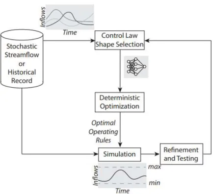
4. PROPOSED PROCEDURE

The main concept behind this thesis work is to apply ISO method to a multi-reservoir system and solve the optimization problem using a GA in order to calibrate the ANN parameters.

Figure 4.1: Schematic representation of the proposed procedure.

4.1 DATASET

As mentioned in chapter 2.4.1, ISO procedure consists of the generation of synthetic data series that allows considering the problem 3.4 as a deterministic one.

Using the models described in chapter 3, a dataset of 1000 years (12000 months) have been generated. The series has been divided into two groups: the first 9000 months have been used to calibrate the parameter, the remaining 3000 months are considered as a validation scenario.

Since the proposed approach does not involve a regression, it was possible to use the 75 years sequence altogether instead of splitting it into smaller series.

(40)

30

4.2 SCENARIOS DESCRIPTION

For this work, four different scenarios have been simulated. The two discriminating factors whose combination give rise to the different settings are the cooperation between the DMs and the quantity of variables used to establish the releases.

The two scenarios that take into account the cooperation between the DMs are defined as centralized, as if one central authority would control the whole system. The situations where the different DMs do not share their knowledge are labelled decentralized.

The scenarios where the only inputs to the model are the water storage and the water demand are called incomplete. If the decision is based on other information as well, it is considered complete.

The variable used as input for each scenario are presented in table 4.1.

Table 4.1: Input variables considered for each scenario. The considered cases are centralized-complete

(CC), centralized-incomplete (CI), decentralized-complete (DC) and decentralized-incomplete (DI). In the centralized cases, the same inputs are applied to all the considered reservoirs, while in the decentralized scenarios the referring reservoir is specified.

INCOMPLETE COMPLETE DECENTRALIZED Roseires 𝑠_𝑡𝑅𝑜𝑠_{, 𝑤𝑑} 𝑡𝑅𝑜𝑠 𝑠𝑡𝑅𝑜𝑠, 𝑤𝑑𝑡𝑅𝑜𝑠, 𝑒𝑡𝑅𝑜𝑠 , 𝑖𝑡+1𝑅𝑜𝑠 Girba 𝑠𝑡𝐾𝑒𝐺, 𝑤𝑑𝑡𝐾𝑒𝐺 𝑠𝑡𝐾𝑒𝐺, 𝑤𝑑𝑡𝐾𝑒𝐺, 𝑒𝑡𝐾𝑒𝐺, 𝑖𝑡𝑢,𝐴𝑡 Nasser 𝑠𝑡𝐴𝐻𝐷, 𝑤𝑑𝑡𝐴𝐻𝐷, 𝑤𝑑𝑡 𝐸𝑔𝑦𝑝𝑡 𝑠𝑡𝐴𝐻𝐷, 𝑤𝑑𝑡𝐴𝐻𝐷, 𝑤𝑑𝑡 𝐸𝑔𝑦𝑝𝑡 , 𝑒𝑡𝐴𝐻𝐷, 𝑙𝑡𝐴𝐻𝐷, 𝑞𝑡𝐷𝑜𝑛 CENTRALIZED 𝑠𝑡𝑇𝑎𝑛𝑎, 𝑠𝑡𝑅𝑜𝑠, 𝑠𝑡𝐾𝑒𝐺, 𝑠𝑡𝐴𝐻𝐷, 𝑤𝑑𝑡𝑇𝑎𝑛𝑎, 𝑤𝑑𝑡𝑅𝑜𝑠, 𝑤𝑑𝑡𝐾𝑒𝐺, 𝑤𝑑𝑡𝐴𝐻𝐷, 𝑤𝑑𝑡 𝐸𝑔𝑦𝑝𝑡 𝑠𝑡𝑇𝑎𝑛𝑎, 𝑠𝑡𝑅𝑜𝑠, 𝑠𝑡𝐾𝑒𝐺, 𝑠𝑡𝐴𝐻𝐷, 𝑤𝑑𝑡𝑇𝑎𝑛𝑎, 𝑤𝑑𝑡𝑅𝑜𝑠, 𝑤𝑑𝑡𝐾𝑒𝐺, 𝑤𝑑𝑡𝐴𝐻𝐷, 𝑤𝑑𝑡 𝐸𝑔𝑦𝑝𝑡 , 𝑛𝑡𝑇𝑎𝑛𝑎, 𝑒𝑡𝑅𝑜𝑠, 𝑒𝑡𝐾𝑒𝐺, 𝑒𝑡𝐴𝐻𝐷, 𝑙𝑡𝐴𝐻𝐷, 𝑖𝑡𝑅𝑜𝑠, 𝑖𝑡𝑢,𝐴𝑡, 𝑞𝑡𝐷𝑜𝑛

4.3 OBJECTIVE FUNCTION

A linear transformation has been applied to the objective vector (3.4b) in order to make the two elements more easily comparable they are normalized and converted to dimensionless values. 𝑱 = [ 𝐽ℎ𝑦𝑑−𝐽ℎ𝑦𝑑 𝑏𝑒𝑠𝑡 𝐽_ℎ𝑦𝑑𝑤𝑜𝑟𝑠𝑡−𝐽_ℎ𝑦𝑑𝑏𝑒𝑠𝑡 𝐽𝑖𝑟𝑟−𝐽𝑖𝑟𝑟𝑏𝑒𝑠𝑡 𝐽_𝑖𝑟𝑟𝑤𝑜𝑟𝑠𝑡−𝐽_𝑖𝑟𝑟𝑏𝑒𝑠𝑡 ] (4.1) Where:

 𝐽_ℎ𝑦𝑑𝑏𝑒𝑠𝑡_{is the annual total amount of energy produced by all the five plants generating}

(41)

31

 𝐽_ℎ𝑦𝑑𝑤𝑜𝑟𝑠𝑡_{is the minimum value (i.e. 0 GWh) that is obtained when there is not any energy}

production

 𝐽_𝑖𝑟𝑟𝑏𝑒𝑠𝑡_{corresponds to the fulfilment of the annual water demand of the five districts of}

the system, the resulting water deficit is 0 km3

 𝐽_𝑖𝑟𝑟𝑤𝑜𝑟𝑠𝑡_{is the sum of the water demands of all agricultural districts throughout the year}

(i.e. 73.3 km3)

The two elements of the normalized vector J (4.1) space in the interval [0, 1] and both of them are to be minimized.

4.4 ARTIFICIAL NEURAL NETWORK

The same ANN architecture has been used for each of the considered reservoir. It consists of a single hidden layer composed by five nodes and a single output regardless of the number of input (fig. 4.2).

Figure 4.2: Architecture of the Artificial Neural Network used.

The parameters that define the ANN have no physical meaning, therefore their upper and lower bounds can be set arbitrarily. In order to guarantee flexibility to the structure, the domain of the parameters is defined to be between -10000 and +10000 (Castelletti et al. 2013).

The same scenarios have been simulated using a linear relationship between the information (It) and the releases (ut) to have a benchmark to compare the ANN with.

⁞

Input layer

Hidden layer