Big data and machine learning for global evaluation of habitat suitability of European forest species

(1)

Big Data and machine learning for

global evaluation of habitat suitability

of European forest species

Teo Beker

Student Id: 876183

Advisor: Prof. Marco Brambilla

Ingegneria Civile, Ambientale e Territoriale

Politecnico di Milano

This thesis is submitted for the degree of

Master of Science in Geoinformatics Engineering

(2)

(3)

(4)

(5)

Acknowledgements

I would like to thank,

my dear family with endless gratitude who supported me, been there for me, helped and guided me throughout my education and life by all means.

my beloved girlfriend Beatrice, for patience and support.

my old friend Marko Arsenovi´c, for introducing me to deeper concepts of neural networks, support, motivation and help in understanding the subject.

my supervisor Prof. Marco Brambilla, for enthusiasm and scientific spirit.

my university, Politecnico di Milano, for providing me the chance to have this experience and get this valuable degree.

to the Institute of Lowland Forestry and Environment in Novi Sad for providing the necessary equipment and especially to PhD Dejan Stojanovi´c for supervision, motivation and daily discussions about technology and science, as well to prof. PhD Saša Orlovi´c for providing a job opportunity in the Institute, professional help, support and great appreciation.

(6)

(7)

Abstract

With the rise in amounts and types of data collected, artificial intelligence and machine learning algorithms have become highly desired. They are being applied in every possible field, for almost every purpose imaginable. In environmental sciences they are applied in remote sensing, in different climate and terrain modeling, even in trait analysis of collected species data. Previous habitat suitability studies using machine learning methods confirmed improvements in results, but until recently it was very difficult to collect or find the data for analysis, and virtually impossible to do such analysis on a large scale. Due to the trend of releasing free global datasets to the public it is becoming possible to do the habitat suitability studies for whole continents or even for the whole globe. Free data sources are analyzed, set of data describing soil, terrain, climate and current distribution of forest species is wrangled and prepared. Habitat suitability study of Fagus sylvatica (European beech) on the global level is performed using machine learning with special focus on artificial neural networks algorithms and big data problem. Results of different algorithms and methods are compared and analyzed.

Keywords: Neural networks; Habitat suitability; Machine learning; Big Data; Fagus Sylvatica;

(8)

(9)

Abstract

Con l’aumento delle quantità e dei tipi di dati raccolti, l’intelligenza artificiale e gli algoritmi di apprendimento automatico sono diventati altamente desiderati. Vengono applicati in ogni campo possibile, per quasi tutti gli scopi immaginabili. Nelle scienze ambientali vengono applicate nel telerilevamento, in diversi modelli di clima e di terreno, anche in analisi di tratti di dati di specie raccolte. Precedenti studi di idoneità all’habitat che utilizzavano metodi di apprendimento automatico hanno confermato miglioramenti nei risultati, ma fino a poco tempo fa era molto difficile raccogliere o trovare i dati per l’analisi, e praticamente impossibile fare tali analisi su larga scala. A causa della tendenza a rilasciare dataset globali gratuiti al pubblico, è possibile effettuare studi di idoneità all’habitat per interi continenti o anche per l’intero globo. Vengono analizzate le fonti di dati gratuite, set di dati che descrivono il suolo, il terreno, il clima e la distribuzione attuale delle specie forestali vengono sballottati e preparati. Lo studio di idoneità all’habitat di Fagus sylvatica (faggio europeo) a livello globale viene eseguito utilizzando l’apprendimento automatico con particolare attenzione agli algoritmi delle reti neurali artificiali e al problema dei big data. I risultati di diversi algoritmi e metodi sono confrontati e analizzati.

Keywords: Neural networks; Habitat suitability; Machine learning; Big Data; Fagus Sylvatica;

(10)

(11)

4.1.1 SRTM . . . 27 4.1.2 ASTER . . . 29 4.1.3 JAXA AW3D30 . . . 29 4.1.4 ISRIC SoilGRIDS . . . 32 4.1.5 Copernicus . . . 39 4.1.6 ICESat . . . 40 4.1.7 Discussion . . . 40 4.2 Climate . . . 41 4.2.1 WorldClim . . . 41 4.2.2 CliMond . . . 46 4.2.3 ECA&D . . . 48 4.2.4 Discussion . . . 50 4.3 Land use . . . 51 4.3.1 FISE . . . 51 4.3.2 Copernicus . . . 54 4.3.3 Discussion . . . 55

5 Integration of big data in habitat suitability modeling 56 5.1 Preprocessing . . . 57

5.2 Data sets creation . . . 59

5.3 Algorithm Choice . . . 62

5.3.1 Ridge and Lasso Regression . . . 63

5.3.2 Logistic Regression . . . 63

5.3.3 Random Forest . . . 63

5.3.4 Gradient Boosting . . . 63

5.3.5 AdaBoost . . . 64

5.3.6 Support Vector Machine . . . 64

5.3.7 MultiLayer Perceptron . . . 64

5.4 Parameter optimization . . . 65

5.5 Rating the algorithms . . . 67

(13)

Contents xiii

6 Implementation 72

6.1 Computing equipment . . . 72

6.2 Data selection . . . 73

6.3 Geographical data preparation . . . 74

6.4 Textual data preparation . . . 75

6.5 Data sets creation . . . 76

6.6 Feature selection . . . 77 6.7 Machine Learning . . . 81 6.7.1 Linear regression . . . 82 6.7.2 Logistic regression . . . 82 6.7.3 Random Forest . . . 84 6.7.4 AdaBoost . . . 86 6.7.5 Gradient Boosting . . . 88 6.7.6 SVM . . . 90

6.7.7 Multi Layer Perceptron . . . 91

7 Experiments 96 7.1 Baselines . . . 96

7.2 Settings . . . 97

7.3 Results . . . 97

7.3.1 Models trained on the forest training data subset . . . 98

7.3.2 Models trained on the whole training data set . . . 102

7.3.3 Visual results . . . 104

7.4 Discussion . . . 108

8 Conclusion 112 8.1 Summary of work done . . . 112

8.2 Contributions . . . 113

8.3 Future Work . . . 114

Bibliography 117

(14)

List of Figures

2.1 Overview of the successive steps of the model building process.[25] . . . . 14 3.1 Top 13 Python Deep Learning Libraries, by Commits and Contributors [10] 26 3.2 Top 8 Python Machine Learning Libraries by GitHub Contributors, Stars and

Commits (size of the circle) [11] . . . 26 4.1 Statistics for the height difference between SRTM and DTED level-2 (Digital

Terrain Elevation Data collected by Kinematic GPS) data for Eurasia. All quantities are in meters. The cell name has the format n(latitude)e(longitude) denoting thesouth-west corner of the SRTM height cell. [52] . . . 28 4.2 Validation results from the Japan study(one arc-second corresponds to 30

meters) [56] . . . 30 4.3 Observation geometries of PRISM triplet observing mode (OB1, left), and

stereo (by nadir plus backward)observing mode (OB2, right).[57] . . . 31 4.4 The status of PRISM stereo scenes in the archive with less than 30% cloud

cover.[57] . . . 32 4.5 Histogram of the height differences from 4,628 GCPs.[63] . . . 33 4.6 Input profile data: World distribution of soil profiles used for model fitting

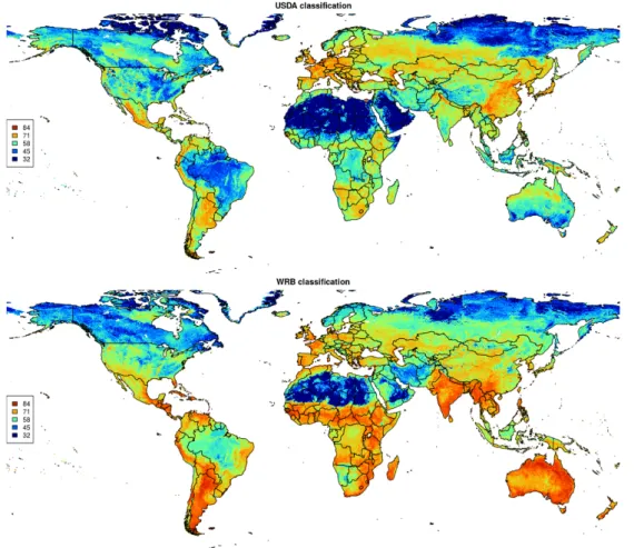
(about 150,000 points shown on the map; see acknowledgments for a com-plete list of data sets used). Yellow points indicate pseudo-observations.[35] 33 4.7 Maps of scaled Shannon Entropy index for USDA and WRB soil

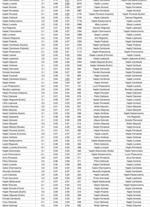
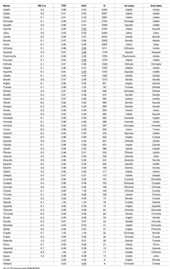
classifica-tion maps. [35] . . . 35 4.8 Classification accuracy for predicted WRB class probabilities based on

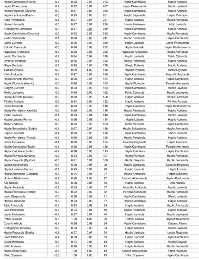
10–fold cross-validation, ordered according to number of occurrences. [35] 36 4.9 Classification accuracy for predicted WRB class probabilities based on

10–fold cross-validation, ordered according to number of occurrences. [35] 37 4.10 Classification accuracy for predicted USDA class probabilities based on

(15)

List of Figures xv

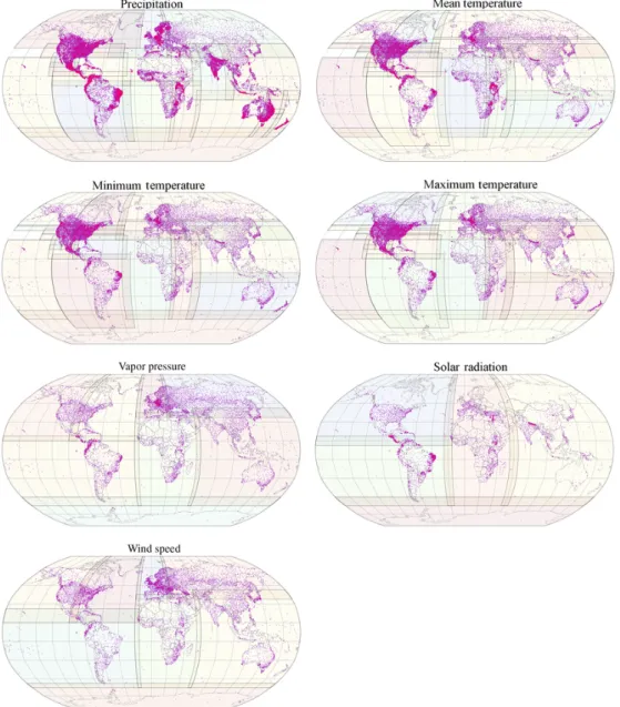
4.11 Spatial distribution of weather stations used for the different climate vari-ables: Coloured boxes indicate boundaries of regions used for creating spline

surfaces. Colour figure can be viewed at wileyonlinelibrary.com. . . 43

4.12 Climate element summary and covariates used in model building. . . 44

4.13 Global twofold cross-validation statistics for selected models. . . 44

4.14 Spatially aggregated RMSE values obtained with twofold cross-validation. . 45

4.15 List of Climond biovariables, with their description and used primary param-eters. . . 47

4.16 Seasonal and annual RMSE and MAE statistics between the 100 reference station values and interpolated values. . . 48

4.17 The location of stations used in the gridding of mean temperature and precip-itation in versions 2.0 (released August 2009) and 16.0 (released September 2017) of E-OBS . . . 49

4.18 The Plot shows the numbers of stations for each month from January 1950 to August 2017.[9] . . . 49

4.19 FISE - Plot density, computed with a spatial grid of 50 km2 . . . 52

4.20 Broadleaved and coniferous forest density . . . 53

6.1 Histogram before undersampling on the whole set, where rpp > 0.0000001 78 6.2 Histogram after limit selection and undersampling on the small subset . . . 78

6.3 Beech layer with relative probability of presence > 0.05 . . . 79

6.6 Correlation heatmap on small subsample with about 120 features . . . 80

6.7 Number of PCA components and explained variance plot . . . 81

6.8 Number of PCA components and explained variance plot at 20 components 81 6.9 Beech density distribution histogram, showing that the data is skewed towards 0 83 6.10 Accuracy of Logistic Regression depending on the C variable . . . 85

6.11 Accuracy of Random Forest model depending on the maximum depth of decision trees and number of estimators variable . . . 87

6.12 Accuracy of Random Forest model depending on the splitting criterion and the number of estimators variable using constant maximum depth parameter 87 6.13 Accuracy of Adaboost model depending on the learning rate and the number of estimators variable . . . 88

6.14 Accuracy of Gradient Boosting model depending on the learning rate and the number of estimators variable . . . 90

(16)

xvi List of Figures

6.15 Accuracy of Support Vector Machines model depending on the regularization parameter C. . . 92 6.16 The comparison of training and validation accuracy of MLP model through

training epochs . . . 95 6.17 The comparison of training and validation loss of MLP model through

training epochs . . . 95 7.1 Comparison of ROC curves of different models on Forest data set . . . 100 7.2 Comparison of ROC curves of different models on whole training data set . 103 7.3 Beech forest distribution map - ground truth (FISE rpp > 0.2) . . . 105 7.4 Comparison of visual results of differently trained models . . . 106

(17)

List of Tables

2.1 Important features to consider when building an HSM, working through the five steps, criteria for detecting potential problems, and some proposed

solutions. [24] . . . 6

5.1 The Differences of the Machine Learning algorithms . . . 64

5.2 Confusion Matrix . . . 68

6.1 Comparison of the specifications of the equipment used . . . 72

6.2 Intel based server data set creation time . . . 76

6.3 Correlation calculation time depending on the data set size. Calculated using Threadripper workstation computer . . . 79

6.4 Ridge regression algorithm accuracy depending on the parameter alpha . . 83

6.5 Logistic regression algorithm accuracy depending on the parameters . . . . 84

6.6 Random Forest algorithm accuracy on Forest dataset depending on the num-ber of estimators parameter and both gini and entropy criterion . . . 86

6.7 Random Forest algorithm accuracy on Forest data set subasample depending on the number of estimators parameter using both gini and entropy criterion 86 6.8 ADAboost algorithm accuracy depending on the parameters . . . 88

6.9 Gradient boosting algorithm accuracy depending on the parameters . . . 90

6.10 Accuracy of support Vector Machine algorithm using linear kernel depending on the parameter C . . . 91

6.11 Support Vector Machine algorithm accuracy depending on the Kernel . . . 92

6.12 Multi Layer Perceptron algorithm accuracy after training on 3 epochs de-pending on the number of neurons and layers . . . 94

6.13 Multi Layer Perceptron algorithm accuracy depending on the learning rate and the regularization . . . 94

7.1 Parameters of the compared algorithms . . . 97

(18)

xviii List of Tables

7.3 Achieved results of the compared algorithms on forest training data set . . . 99 7.4 Feature importance extracted from each model trained on the forest training set101 7.5 Achieved results of the compared algorithms on whole training data set . . 101 7.6 Achieved results of the compared algorithms on whole training data set . . 102 7.7 Feature importance extracted from each model trained on the whole training

data set . . . 104 7.8 Accuracy metrics of the algorithms trained on forest or whole set, used for

generating the habitat suitability map on whole Europe . . . 108 7.9 Achieved confusion matrix results of the compared models, trained on both

training data set, predicting whole European data set . . . 108 A.1 List of Layers used . . . 122 A.1 List of Layers used . . . 126

(19)

Chapter 1 Introduction

1.1 Context

Since the dawn of time, humans have been surrounded by data. Little by little it has become more structured and we could deal with larger amounts of diverse information. Now in information age, we have ability to record and measure large amounts of data without the need of spending people’s time. It is becoming of importance to process ever larger amounts of recorded data and to extract the meaningful information out of that. This has marked the rise of data science as the most demanded and sought after discipline in the last decade.

The biggest concern of 21st century is global warming, and the climate change which we have imparted on ourselves. The changes that climate is making are threatening to seriously disturb the global biosphere by pushing moderate climate further from the equator at previously unseen speeds. These changes on continental surfaces can affect the forests significantly since forests cannot naturally follow the gradient of climate change. They grow and spread very slowly. Also forests are the bases of many ecosystems and if forests die off, the large parts of ecosystems will be highly affected too. This means that large effort should be made to research the forests species suitable environmental ranges, and define endangered zones. With these zones and ranges defined, plans for change of forest species or for potential mitigation can be created and enacted.

The field that deals with habitat suitability models of ecosystems is called bio-geographical modeling, and so far there have been created many models which implement future climatic scenarios to make predictions. Although use of more complex data science tools have been very rare. One of the reasons of this is that the more complex the algorithm the less inter-pretable it is. It is very good to work with interinter-pretable models, it can give us many insights into data, confirm or imply new theories, but this does not guarantee the complete use of data, extraction of all the potential. Neural networks have managed to surpass expectation of

(20)

2 Introduction

many, they often can give highly accurate predictions, or can imply unexpected underlying patterns. On the other hand, they are very difficult for the interpretation, and they are often used as black boxes. As a result they have not seen much use in bio-geographical modeling until now.

There have been a lot of efforts directed at gathering and processing geographical data such as climate, terrain, soil characteristics, species locations, and classifications... With rise of satellite remote sensing such data is becoming more easy to gather and to generate. Still soil data is very difficult to come by, since it implies manual labour and digging of the holes, and is lacking in its accuracy and resolution on wider scales. There have been efforts to collect and process the available soil data on global level and to generate global soil maps. Recently there have been some new data sets released to public, such as SoilGRIDS. It has been generated at 1km resolution at first, and later at 250m, with a goal of reaching 30m in the future. Climate models have been calculated for long times now, and they are available in many different shapes. There are futuristic models available for use also. The terrain data generated by geodetic surveys has recently been unified and published at coarse resolution free of charge. Soon after that satellite surveys have overtaken them in global accuracy (On local level geodetic surveys are extremely precise). All of this independent data is improving slowly and becoming more precise as the new data becomes available and gets included in the models. This is a point in time when global geographic data analysis is becoming widely possible, to individuals as well as to well-established research facilities.

Today it is a question of using this knowledge and data for developing models which can help deal with problems by generating new insights and useful information. By using the soil, climate, terrain and forest data we can efficiently on much higher level make habitat suitability models for forest species at different time intervals or different futuristic scenarios. Even though some of the data is not the most precise at this point of time, the promise of improvement is enough to start developing the procedures for such model generation.

1.2 Objective

Since this is a new field of research and there is not a proposed methodology of work, the aim of this thesis would be to supply an approach to big geographical data habitat suitability analysis using data science tools. As it always is with all things new, the basics need to be set first, which is the reason why the objectives of this thesis are the following:

• Can we use available geographic data in big data context efficiently? • How to measure the level of generalization of the models achieved?

(21)

1.3 Proposed Solution 3

• Do differently created training data sets improve the accuracy of the models? • Do additional data sets improve the accuracy of the models?

• How to deal with huge amounts of data and big data problems that arise in the process? • Is higher complexity too high a price for the reached accuracy?

• Which are the optimal machine learning and deep learning algorithms for these pur-poses?

Those are just some of the questions that need to be answered along the process of automating generation of such models.

1.3 Proposed Solution

The goal of this thesis is to present procedures for generating global habitat suitability analysis using advanced machine learning algorithms for European forest species, especially European beech. The developed procedure can later be translated and adapted to other species and used for futuristic climate scenarios analysis.

This kind of study has been done in the past using limited data and simple regression algorithms. Now it is possible to get the huge amount of geographic data and do the big data analysis. This complicates the traditional modelling approach and asks for data science approach to be used.

Data science is multi-disciplinary field that uses statistical methods, algorithms and systems to give insights and knowledge about the analyzed data. The data analyzed can be highly structured or completely unstructured. Data science has two subfields: Data Mining which focuses on detecting the patterns in the data and big data which deals with data that is too large to be processed using traditional systems. The definition of where is the limit when data begins to be big data is still vague, but it is becoming widely accepted that limit is the data that is larger than the computer operational memory size.

To deal with huge amounts of unknown data, data science uses statistical approaches -machine learning algorithms and effective visualizations to explore it and to find underlying patterns. To be able to apply the machine learning algorithms the data preparation process must be performed. The data needs to be structured, the missing values filled or eliminated and variables explored and chosen which to use for the problem at hand. Most often this process takes the most time, theoretical ratio is 80% of time goes for data preparation and 20% to data analysis.

(22)

4 Introduction

Geographical data generally falls in the more structured data, which simplifies some steps in the data preparation process, but big data problems prevail. Also the geographical data has its own characteristics which need to be addressed first. The reference system, spatial resolution and area need to be equalized. After that the data is transformed into textual format to be further processed in data science fashion.

The available free open source data is explored and compared. The chosen data needed to be analyzed and merged into usable data set. The approaches for the training data set generation are compared. The approaches are tested out using different algorithms on the area of European continent.

The different machine learning algorithms are also compared during this process on the accuracy metrics, confusion matrix, precision, recall and time of execution on two created data sets. Resulting maps are compared. Conclusion on on usage of machine learning algorithms and the creation of training data set is made.

The goal is to generate the predictive model of habitat suitability for European beech. Because of global scope of this study and reasons mentioned in the chapter about habitat suitability modeling we will focus on abiotic environment. Also since the habitat suitability models are done for the forests, which can easily be planted by humans, it is considered that the species has the absolute dispersal capacity. Results of such habitat suitability study should show where the forests could be, not where they will be in foreseeable future.

1.4 Structure of the Thesis

The structure of this thesis is as follows:

• Chapter 2 describes the background of the field of habitat suitability modeling which will be performed in this thesis.

• Chapter 3 compares the python software libraries which are used for machine learning and neural network applications, and discusses them.

• Chapter 4 describes the available data sets and the reason why are ones chosen over the other.

• Chapter 5 contains the description and outline of the process of creating the data sets and the analysis performed in this thesis.

• Chapter 6 describes the implementations of the procedures.

(23)

1.4 Structure of the Thesis 5

• Chapter 8 concludes this report by summarizing the work, doing a critical discussion and advises the possible future work.

(24)

Chapter 2 Habitat suitability modeling

Habitat suitability models are empirical methods that relate species’ distribution in sampled areas with environmental habitat feature data by using statistical and theoretical calculations to give a representation of the species’ environmental niche. It has greatly developed and become much more used in last few decades because it has been supported by the technological advancements, mainly increase in computing power, ability to gather data faster (for example remote sensing) and wider availability and accessibility of species distribution data (Digitalization of museum samples and other biological collections).

Habitat suitability modeling should follow the next 5 steps (Figure 2.1) [25]: 1. Conceptualization

2. Data preparation 3. Model calibration 4. Model evaluation 5. Spatial predictions

The detailed process consists of many steps which are presented in the Table 2.1 taken from [24].

Table 2.1 Important features to consider when building an HSM, working through the five steps, criteria for detecting potential problems, and some proposed solutions. [24]

Begin of Table 2.1 Feature to consider Possible problems Detection criterion Examples of proposed solution 1. Conceptualization (conceptual model)

(25)

7 Continuation of Table 2.1 Feature to consider Possible problems Detection criterion Examples of proposed solution Type of organism Mobile species in unsuitable habitats Radio-tracking; continuous time field observations Neighborhood focal functions; choice of grain size Sessile species (e.g. plants) in unsuitable habitats Lack of fitness (e.g. no sexual reproduction) Use fitness criteria to select the species observations to be used in model fitting Species not observed in suitable habitats Knowledge of species life strategy (e.g. dispersal) Interpret the various types of errors Low detectability species Field knowledge, literature

Correct test for detectability Sibling species or

ecotypes in the same species

Genetic analyses Test niche-differentiation

along environmental

gradients Invasive species Mostly

commission errors

Fit models in the area of origin Type of predictors Direct or indirect predictors Ecophysiological knowledge Avoid indirect predictors

(26)

8 Habitat suitability modeling Continuation of Table 2.1 Feature to consider Possible problems Detection criterion Examples of proposed solution Type of model needed Need to include environmental or biotic interactions, dispersal, autocorrelation, abundance, etc. Ecological theory and available data

Consider an HSM technique which

takes these features into account (e.g. tree

based for abiotic interactions, spatial autologistic for autocorrelated data) Designing the sampling Selecting sampling strategy Simulation tests with virtual species in a real landscape Random or random stratified(by the environment) sampling Incorporating ecologi-cal theory Linear or unimodal response of species to the predictors Partial plots, smoothing curves Generalized additive model (GAM) or quadratic terms in generalized linear model (GLM) Skewed unimodal response curves

Skewness test HOF, beta functions in GLM, GAM, fuzzy envelope

(27)

9 Continuation of Table 2.1 Feature to consider Possible problems Detection criterion Examples of proposed solution Bimodal response curves Smoothing curves, partial plots GAMs, ≥ third-order polynomials or beta functions in GLMs 2. Data preparation (data model)

Species data Bias in natural history collections (NHC) Cartographic and statistical exploration Various ways of controlling bias Heterogeneous location accuracy in NHC Only detectable if recorded in the database Selecting only observations of known accuracy below the threshold No absences Type of database

and source (metadata) Generating pseudo-absences Environmental predictors Errors in environmental maps Cartographic and field-proofing exploration Incorporating error into the

models Missing key mapped environmental predictors Ecological theory or reduced variance explained remote-sensing (RS) data as an alternative source Scale (grain/extent) Different grain sizes for the various predictors

GIS exploration Aggregating all GIS layers at the

(28)

10 Habitat suitability modeling Continuation of Table 2.1 Feature to consider Possible problems Detection criterion Examples of proposed solution Truncated gradients within the considered extent Preliminary exploration of species response curves Enlarging the extent of the study area to cover full gradients 3. Model fitting Type of data

No absences Type of database and source (metadata) Using profile methods Multicollinearity Correlations between the predictor variables Variance Inflation Factor (VIF) Removing correlated predictors; orthogonalization Spatial autocorre-lation (SAC) Non-independence of the observations

SAC indices Resampling stratefies to avoid SAC; correcting inference tests and possibly incorporating SAC in models Type of statistical model

Oversdispersion Residual degrees of freedom > residual deviance Quasi-distribution in GLMs and GAMs; scaled deviance

(29)

11 Continuation of Table 2.1 Feature to consider Possible problems Detection criterion Examples of proposed solution Model selection Which approaches and criteria? - AIC-based model averaging; cross-validation; shrinkage 4. Model evaluation Type of data No absences; usual measures not applicable Type of database and source (metadata) New methods emerging for evaluating predictions of presence-only models (Boyce index, POC-plot, MPA, area-adjusted frequency index) Evaluation framework No independent set of observations - Resampling procedures Association metrics Choice of a threshold for evaluation - Threshold independent measures (AUC, max-TSS, max-Kappa, etc.)

Error costs - Error weighting

(e.g. weighted Kappa) Model uncertainty Lack of confidence Uncertainty map, residual map Bayesian framework; spatial weighting

(30)

12 Habitat suitability modeling Continuation of Table 2.1 Feature to consider Possible problems Detection criterion Examples of proposed solution Model selection uncertainty Lack of confidence Comparing selection algorithms and completing models Model averaging, ensemble modeling Spatial predictions: Projection into the future and in

new areas Range of new predictors falls outside the calibration domain Statistical summaries Restrict area of projection; control the shape

of response curves 5. Spatial predictions and model applicability

Scope and applicability Model not applicable to a distinct area Unrealistic response curves Avoid overfitting Problem of future projections HSMs not transposable to distinct environments Strongly dependent on the scale considered spatially explicit models incorporating population dynamics, dispersal and habitat Use in management Difficult to implement in a management context Software not available to managers and decision makers Free software

(31)

2.1 Overview of habitat suitability principles and theory 13 Continuation of Table 2.1 Feature to consider Possible problems Detection criterion Examples of proposed solution Not interpretable Black-box

algorithms? Coice of easy-to-read and easy-to-interpret methods (GLMs, GAM, CART)

2.1 Overview of habitat suitability principles and theory

When doing the habitat suitability model, it should be started with conceptual design. First the scientific question to which habitat suitability model should give an answer needs to be formulated, as well as objectives of the modeling. Secondly, the model which will be used should be picked and conceptually presented based on ecological knowledge, then have defined the assumptions made when building the model, and finally define the parameters used for model prediction.

Sampling strategy for the species observations if necessary should be well defined. And spatio-temporal resolution of the data gathered or used should be chosen. Species data can be defined differently: presence, presence-absence or abundance observation, all of which can be sampled randomly or by stratified sampling. Opportunistic sampling could be set as a separate category, where the data is collected from different collections (museums, online biodiversity databases, etc.) and sampling strategy or uniformity cannot be guaranteed.

After the goals and data gathering have been properly defined, modeling methods should be taken into consideration. The most adequate methods should be identified, depending on the goal of the model and type of data available, as well as evaluation framework for estimating the validity of the model as well as statistical accuracy.

In conceptual phase other features might be necessary to consider also, depending on the project and analysis planned to be performed. It should all be done as early as possible, though often not everything is known from the beginning and therefore some things are unable to be planned for from the start.

For a species to occupy certain location and to maintain populations three main conditions need to be satisfied [48]:

(32)

14 Habitat suitability modeling

Figure 2.1 Overview of the successive steps of the model building process.[25]

• Abiotic environmental conditions must be appropriate for the species (Abiotic habitat suitability)

• Biotic environment must fit the species (Biotic interactions)

At continental and global scale it is very difficult to model the biotic factors for the species. It is very rare that biotic factors - species interactions completely override abiotic suitability. Especially on large scale it appears that distributions of almost all species seem to be determined by the abiotic environment, particularly climate [2].

Also important factor in species-environment responses is spatial resolution used. The species distribution can change by changing the resolution used, as shown in study [18]. Also, there were noted other considerable differences in results received from 4km, 800m and 90m models.

Formation of new and distinct species through evolution is called speciation. Two most common types of speciation are allopatric (influenced by gene pool limitation directly) and symaptric speciation (influenced by different paths of evolution of the same species). Allopatric speciation happens when geographic barriers divide one species into two or more disconnected groups, leading to dividing of the gene pool and ultimately to speciation into distinct taxa [29]. Sympatric speciation arises when the species goes in different directions of development often due to ecological specialization for different environmental conditions. For habitat suitability modeling it is important to know that this happens at a slow pace and the be aware of consequences that the speciation has when modeling past or future scenarios.

(33)

2.1 Overview of habitat suitability principles and theory 15

When we look at today species distributions, we can see that many species are limited to certain areas, often ones where they originated. Dispersal and geographic origin of the species play a huge role when we analyze current species distributions, even bigger than environmental suitability. From this it can be concluded that an absence of a species does not have to mean that environment is not suitable for it but dispersal limitations might have played a big role also.

It was detected by the early biogeographers that some species occurred in different environmental conditions, while others could only occur in highly specific environments. It lead them to form the theory that each species can inhabit a range of conditions along the environmental gradients to which they have physiologically adapted through evolution. The environmental gradient at which the species performs the best, at which it reaches the physiological optimum, usually features the most or the most prominent examples of the species, and the further away from the optimum, the performance declines. Such physiological response curves usually have the unimodal or sigmoidal shape. The width of the curve demonstrates the resilience of the species to the change in environmental gradient.

Each species depends on different environmental factors, and many of them. To some it is more resilient, to others not, if looked at separately combined effects might be missed. Because of that, when modeling, it is of importance to consider all the important variables jointly to define the environmental niche of the species [22]. Environmental Niche is quantitatively defined as: jointly considered physiological responses of a given species to several environmental variables which define multidimensional volume - fundamental environmental niche [30]. When the fundamental environmental niche is constrained by the biotic relations, we get the realized niche.

To model with high accuracy and confidence it is important to know which variables directly affect the species. To find out which variables are these, it is required to do ex-perimental lab tests, which can be costly and consume a lot of time. It is not viable to do this for large numbers of populations for all species. Because of this it is common to use environmental measurements that are hypothesized to affect the species. Although, doing this reduces the predictive power of the model.

Biotic environment plays a big role in species inhabiting certain area, or even species dispersal. First example of biotic factor is competition when two species occur at the same location and compete for the same limited resources, less competent species will ultimately be excluded, this principle is called "competitive exclusion principle" [54]. Evidence of this can be observed at local scales, but the study [21] it can be also detected at larger scales.

If species cannot be found in certain gradient the observations will give incomplete picture of a full physiological response, since it can be influenced by biotic factors. This type

(34)

of field data observations along a single gradient is called ecological response or realized response. Opposite of this is physiological response or fundamental response which observes species without biotic interactions. Same as fundamental niche is created using fundamental or physiological response, realized niche is modeled using realized response.

Asymmetric abiotic stress limitation hypothesis states that ranges of specis along en-vironmental gradients tend to be limited by physiologically more stressful edge, and by competitive interactions toward physiologically less constraining and more productive parts of environmental gradient [41].

Biotic interactions can be positive and negative. Examples of positive biotic interactions feature commensalism, mutualism, biotic engineering (species improving the micro habitat conditions for another) [37]. Negative interactions include competitive exclusion, predation (for example herbivory) and parasitism (when host is affected by parasite to complete exclusion). Such interactions can be used as variables for species distributions modeling.

There are other views of the niche, but main two are: the one that has been described, Hutchinson’s, niche determined by environmental requirements of the species, and the second one determined by the species’ functional role in the food chain and its impact on the environment, by Elton’s definition. Both concepts are relevant, but often they are taken separately into consideration. Late studies have linked the food webs with habitat distribution modeling showing the two concepts are entwined [46].

2.2 Approaches to modeling

The field of biogeographic modeling has three approaches: descriptive, explanatory and predictive. Descriptive models are made to get an insight into the parameters surrounding the species or ecosystem, explore the links between for example species occurrence and other potentially meaningful variables. Explanatory models by using prior knowledge of a system, aim to validate a certain hypothesis. Predictive models are the models that obtain the best fit. They often can lead to biased parameters and in favor of a smaller variance. So it does not explain the ecological data the best but gives the best predictions. Here the most diverse set of algorithms can be used.

Ultimately biogeographers should aim for explanatory models that at the same time offer good predictive performance, in practice, there is a trade-off between explanatory and predictive power [25]. Even though this problem has been explored for a long time in biogeographic modeling, it has shown that not all algorithms can deal effectively with this trade off [40].

(35)

2.3 Types of algorithms used 17

2.3 Types of algorithms used

2.3.1 Regression based approaches

Regression based algorithms are the most used algorithms in biogeographical modeling and ecology in general. They rely on robust statistical theory and are easily interpretable [23].

Regression statistically relates the wanted response variable (in case of biogeographic modeling it is presence, presence-absence or abundance information) to a set of environmental variables. The ordinary least square linear regression is used only when the response variable is normally distributed, and variance does not change as a function of mean.

Generalized Linear Models (GLM) are a more flexible group of linear regression models which is more flexible to the distributions and variance functions of the response variable. Generalized linear models connects the predictors to the mean of response variable using link functions. This makes it possible to transform the response to linear space and keep the predicted values within the range of values allowed for response variable. By doing this it can deal with Gaussian, Poisson, binomial or gamma distributions by setting the link functions to identity, logarithm, logit and inverse, respectively [24]. If the response has a different distribution, higher order polynomial term of predictor can be used, and this is called polynomial regression.

Generalized Additive Models (GAMs) are designed to use the strengths of generalized linear models without requirement of defining the shape for the response curve from specific parametric functions. They use smoother algorithms to automatically fit the response curves, according to the set smoothness parameter. This helps when the relationship between the variables has complex shape, or where the shape is unknown. Because of this the generalized additive models can be used for exploration of the shape of response, before using other models for fitting.

Multivariate Adaptive Regression Splines (MARS) are more flexible regression technique than generalized linear models because they do not require the assumptions about underlying functional relationship between the species and the environmental variables. It can model the nonlinear responses. It splits the output into multiple broken segments, connected by knots, of which each has different slope. When the model is fitted there is no break in the function or abrupt steps.

2.3.2 Classification based approaches

Classification approaches, recursive partitioning and machine learning approaches fall in the group of supervised learning and classify observations into homogenous groups. Cluster

(36)

analysis is a form of unsupervised learning which is most widely used approach to group the observations, based on one or more variables.

Examples of the classification algorithms used in biogeographical modeling are: Discrim-inant analysis [27], Recursive partitioning [6] [49], support vector machine [13] and there have been attempts at using neural networks [51] [17]. The conclusion was that classification methods are not necessarily better than regressions, but they may offer easy understanding and nice representations in a very informative format like recursive partitioning, or reveal some properties previously undetected [24].

Recursive partitioning is probably the classification algorithm of largest interest for habitat suitability modeling. It is very easy to explain and interpret, and results can be presented in a decision tree which is very intuitive in itself, showing the interactions between variables. It can be used in more complex algorithms by being a building block of meta-algorithms like boosting and bagging for example. It can deal with discrete or with continuous response, in first case it would be called classification trees, in second regression trees. The decision tree is produced by splitting the data by a rule based on single variable repeatedly until the satisfactory model and accuracy are achieved. At each splitting node data is split into two groups. Recursive partitioning does not rely on assumptions about the relationship of the response and the variables, and it does not expect the variables to follow any distribution which are significant advantages of this model.

Artificial Neural Networks (ANN) is an algorithm inspired by the biological neural system, its interconnected neurons. It uses automatically trained adaptive weights which numerically define the strength of signal sent to the next neurons. By doing this it can model very complex nonlinear functions. They can handle any type of a variable, continuous, discrete, Boolean and do not assume the normal distribution of the data. They are robust to noise [12], and generally achieve very high accuracy [36] [38] [44] [65]. Even though it has all these benefits it has not been used much in ecology. It is not interpretable easily, it lacks transparency, the difficulty to implement them correctly and their stochasticity are main reasons why they have not seen much use in ecology yet.

2.3.3 Boosting and bagging

Bootstrap AGGregation or bagging is a meta-algorithm approach of using multiple randomly subsampled with replacement samples (bootstraps) from the used data set, and a different model is trained from each bootstrap. In the end the results are combined in a way, usually using the mean or mode of the results. This procedure significantly reduces the variance of the prediction. The most famous example of bagging algorithm is random forest [5].

(37)

2.3 Types of algorithms used 19

Boosting is another ensemble meta-algorithm approach which uses more complicated stage-wise procedure to improve the predictive performance of the models. The models are fitted sequentially to the data, each iteration fitting to the residuals of the previous one. This is repeated for defined number of times until the final fit is made. There are different ways to implement this, and it can be used on different models. It has been suggested to use the stochastic gradient boosting to improve the quality of the fit and avoid overfitting [19]. Boosted regression trees belong to this category.

(38)

Chapter 3 Processing tools

3.1 GDAL

Geospatial Data Abstraction Library (GDAL) is open-source software library for geospatial data processing. It originated in 1998 and has been developed and improved significantly since. It is written in C++ and C for use and processing of raster and vector data (OGR part). It comes with an command line utilities and an API.

It is currently one of the key open-source software packages for geospatial data processing. It is used in many open-source software projects: QGIS, GRASS, MapGuide, OSSIM and OpenEV, and even to varying degree in some proprietary: FME, ArcGIS, Cadcorp SIS... [20] GDAL is closely aligned with OGC standards, and while offering wide options is designed with simplicity in mind. When opening files, it is not needed to know which format it is, software recognizes it alone, each of the format drivers are given a chance to try and open the data set.

It is available for Windows and any POSIX compliant operating system. Mac OS versions before X are not covered, but MacOS X and later versions are. Being written in C and C++ was a success, because of the stability, speed and community support. Many of proprietary software vendors which use and financially support GDAL project are themselves building C/C++ applications, if GDAL was written in other languages it probably would not have been viable for them to use and support it. Being written in C/C++ made it easy to wrap it using simplified wrapper and interface generator (SWIG) to make it available in other languages Python, Perl, C# and Java. All these characteristics helped GDAL achieve one of its goals, ubiquity.[68]

GDAL has done significant work in making the code Thread Safe, but still there might be drivers with missing support, .vrt for example. Using terminal many functions still work on a single CPU core, but some allow use of more than one core.

(39)

3.2 Python - Jupyter Notebook 21

It is released under MIT/X license, which allows licensee to copy, modify and redistribute the licensed code as long as the copyright is notice on the code is not changed and the disclaimer of warranty is accepted.

3.2 Python - Jupyter Notebook

Python is an interpreted high level programming language, created in 1991 by Guido van Rossum. It has become one of the main languages used in scientific community for dealing with wide range of tasks. Also lately with a rise of the Data Science it has taken the main role in data analysis and prototyping.

Python has a wide range of free libraries to use, almost for any purpose. There is a good common selection of libraries for computation and for use in data analysis. Some of them are numpy, pandas, scykit learn, tensorflow, keras, neon, theano, caffe, pytorch, matplotlib which will be described later.

Jupyter Notebook was developed in 2015 by Jupyter Project, a nonprofit organization. Its name is given in homage to Galileo’s notebooks recording the discovery of the moons of Jupyter, and as a reference to supported core programming languages: Julia, Python and R. It is based on IPython (Interactive Python) which offered interactive shells, a browser based notebook interface, support for interactive data visualization, embeddable interpreters and tools for parallel computing.

The development of Jupyter has started with a goal of making scientific computation more readable, more understandable to humans. The way to do this was through computational narrative, to make a computations embedded in the narrative that tells the story to particular audience. To achieve this three main aspects were considered [47]:

• Single computational narrative needs to span a wide range of contexts and audiences, • Computational narratives need to be reproducible and

• The collaboration in making computational narratives needs to be easy.

The idea of interactive computing is at the core of the Jupyter, users executing small pieces of code and immediately getting the results. This is of most importance in data science, since data exploration bases its next step on the results of the each step before. To achieve this architecture for interactive widgets and user interface and user experience have received a lot of attention.

Collaboration improvements have been approached very seriously. There were a few improvements in this area, where real time collaboration played a significant role. It was

(40)

22 Processing tools

desired to make Jupyter easy for more people to collaborate on at the same time. Google Drive was used as an example, where simultaneously more people could access, change and see the changes, comment and share the document. These ideas resulted in Jupyter Hub, the notebook server.

It is becoming more common to include the notebooks with scientific papers, for the reproducibility of the analysis. The web platform, Binder, has been created for running the notebooks from GitHub online. Jupyter notebooks can easily be converted using nbconvert to other formats such as Latex, HTML or PDF. Books have been written and printed as a collection of Jupyter notebooks. Jupyter is slowly being adapted for writing academic papers as notebooks. [33]

Success of this project is obvious, today it has become widely used platform for scientific programming and data science in particular. Ease of programming, ability to give context to calculations, simple and effective user interface and wide support of community and online tools for Jupyter notebooks make this a very compelling environment for academic and Data Science projects.

3.2.1 NumPy

NumPy is a successor to Numeric and Numarray libraries. It was published in 2006 by Travis Oliphant with a goal to create a basis environment for scientific computing. [42] It is open-source module for Python which provides mathematical, numerical and matrix and large arrays manipulation functions.

It is primarily useful for NumPy array format which is a multidimensional uniform collection of elements. It is characterized by the type of elements it contains and by its shape. It can have any dimensionality and can contain any type or combination of types of elements.[67]

3.2.2 Pandas

Pandas is a Python library for data manipulation and analysis with performance optimization. It was released in 2008, authored by Wes McKinney. Its name is derived from Panel Data, which is a term used in statistics and econometrics for multidimensional data sets.

It adds DataFrame format which allows users to label the matrices and multidimensional arrays. Also it includes functions for grouping and aggregating data into pivots or contingency tables, automatic data alignment, hierarchical indexing, data filtration, and many other options for data manipulation from different angles. [39]

(41)

3.2.3 Scikit-learn

Scikit-learn is a free open-source Python library for machine learning, designed to work with NumPy and SciPy libraries. It was developed by David Cournapeau and realeased in 2007. Its name is derived from the notion that it is SciPy toolkit, "SciKit".

It includes compiled code for efficiency, it only depends on Numpy and Scipy, and it focuses on imperative programming. It is written in Python, but it includes some C + + libraries, like LibSVM for support vector machines. A lot of attention has been given to quality and solid implementations of the code and as well as to consistent naming of functions and parameters, according to Python and Numpy guidelines.

Scikit-learn is mostly written in high level language and focuses on ease of use, but it also showed big speed improvements as well as ability for more control in defining machine learning parameters for some of the algorithms in comparison to its predecessors. [45]

3.2.4 TensorFlow

TensorFlow is a symbolic math, free, open-source software library. It is written in Python, C+ + and CUDA and used for machine learning and especially for neural networks. It was developed by Google Brain team and released in November 2015. It was based on DistBelief also machine learning library developed by Google.

TensorFlow uses unified dataflow graphs for computations in an algorithm and the state on which the algorithm operates. It has deferred execution, which means it has two phases: definition of a program as a symbolic dataflow graph with placeholders for the input data and variables that represent the state and second which executes an optimized version of the program on the set of available devices. It also features optimizations for CPUs, GPUs and also TPUs.[1]

Currently TensorFlow is the most popular library for Neural Networks, it has the biggest user community, it is very well documented and has good support. It is often considered as the best library to start learning to use Neural Networks.

3.2.5 Keras

Keras is an open-source library written in Python for application of neural networks. It’s primary author is François Chollet, a Google engineer. It was released in 2015. It’s aim is to be easy to use, modular and extensible. Models are created as a sequence or as a graph - as TensorFlow. It was intended more as an interface (middleware) than independent

(42)

24 Processing tools

framework.[8] It supports TensorFlow from the beginning, and later it had support for CNTK, Theano and PlaidML added.

Keras is very good for the simplicity readability and a very smooth learning curve in comparison to other libraries. That is the reason why it is often recommended for beginners and simpler projects. In 2017 Keras reached over 200 000 users. Because of simplicity and such popularity there is a lot of material available about using Keras on Neural Networks [26].

3.2.6 Neon

Neon is Intel Nervana’s open-source deep learning framework. It was designed with prime goal of high performance, and secondary goals of ease of use and extensibility. It boasts to outperform rival frameworks such as Caffe, Theano, Torch and TensorFlow. The high performance advantage is achieved due to assembler-level optimizations, multi gpu support and through smart choices in the algorithms. It has high level API structure which is similar to Keras.

Because of its speed, simplicity and similarity to Keras as well as good support and large model zoo it is gaining in popularity. It is continuously improved. Intel states that improvement in speed between versions 2.4 and 2.6 on Intel server platforms amounts up to 7.8 times. Intel’s analysis shows that in some cases neon framework can be faster up to 50% in comparison to other mentioned frameworks.

3.2.7 Theano

Theano is a free open-source Python library for definition, optimization and evaluation of mathematical expressions. Theano syntax is very similar to the syntax of Numpy and is compiled to run efficiently either on CPU or GPU. It was initially released in 2007 by Montreal Institute for Learning Algorithms under BSD license.

Theano was first to implement many of the technologies which are now widely used in machine learning research libraries. For example: combining high level scripting language with highly optimized computation kernels, use of GPU in computations, computation graphs, automatic generation and compilation of kernels and graph rewriting and optimization are widely used today.[64]

(43)

3.2.8 Caffe2

CAFFE (Convolutional Architecture for Fast Feature Embedding) is a free open-source deep learning framework for use with multimedia. It was developed by Yangqing Jia from 2013 at University of California, Berkeley and released under BSD license. Caffe2 was released in 2017 and one year later it was merged into PyTorch. It was written in C++ with Python and Matlab bindings.

Caffe is made with primary concerns for expression, speed and modularity. It was designed for computer vision, but has been also used and improved for speech recognition, robotics, neuroscience and robotics.[31] It is one of the fastest and most used frameworks for deep neural networks today.

3.2.9 PyTorch

PyTorch is an open-source machine learning library for Python, based on Torch. Torch was released in 2002 and PyTorch has been developed by Facebook’s AI research group and initially released in 2016 [43]. Caffe2 was merged into PyTorch in 2018 as a result of ONNX (Open Neural Network Exchange) project.

PyTorch was built with an aim to be flexible, fast and modular. It has hybrid front-end which allows it to seamlessly transition to graph mode and back, its back-end is made for scalable distributed training and it has a rich ecosystem with a lot of libraries, tools and other content to support development. [32]

3.2.10 Discussion

For preparation of the data numpy, pandas and visualization libraries like matplotlib and seaborn have proved indispensable. For machine learning purposes the library that is the most widely used, with very high number of contributors and commits is scikit-learn which can be seen on the Figure 3.2. This "popularity" will be very helpful when encountering difficulties and problems with coding, because solutions of many problems are already defined. Therefore this library has been chosen to be used for this study.

The same approach for choosing the deep learning libraries is used. Here Keras and TensorFlow are in absolute lead with general usage according to the number of contributors and commits published by KDNuggets (as can be seen on the Figure 3.1), thus they are selected to be used.

(44)

26 Processing tools

Figure 3.1 Top 13 Python Deep Learning Libraries, by Commits and Contributors [10]

Figure 3.2 Top 8 Python Machine Learning Libraries by GitHub Contributors, Stars and Commits (size of the circle) [11]

(45)

Chapter 4 Data overview

4.1 Surface and Soil

4.1.1 SRTM

The Shuttle Radar Topography Mission (SRTM) was an 11 day mission in February 2000 based on Space Shuttle Endeavor and C/X band Synthetic Aperture Radar. It globally collected the elevation data which was later processed and in 2003 released to the public as the first free global digital elevation model. It was anticipated to have the 30m pixel spacing and 15m vertical accuracy [15]. At first it was only released in 3 arc sec (about 90m) resolution, and in 2015 the 1 arc sec (about 30m) spatial resolution data was published. It covered the globe from 60 degrees north to 56 degrees south latitude.

Since publishing, it has went through couple of versions. In version 2 substantial editing has been performed and the results exhibit well defined coastlines and the absence of spikes and wells, but still there are some areas which have missing data (Voids). Additional coastline mask is included with the vector data.

Version 3 or SRTM-plus develops on version 2 and voids are filled with ASTER GDEM2 data and in small measure using US Geological Survey data.

The data has been used for different purposes, even the global bathymetry was developed from the data collected by SRTM and other missions.

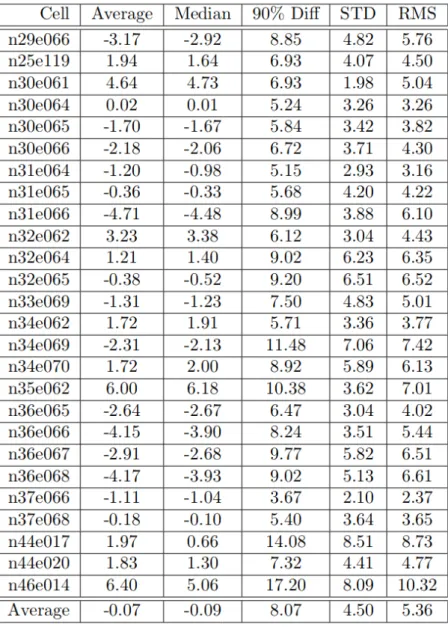
Much research has been done to estimate the accuracy of the SRTM data. All studies confirm the accuracy is higher than anticipated with results often satisfying accuracy lower than 10m RMSE even in some plane areas of 5m RMSE [52]. The absolute and relative height accuracies are estimated to 9 m and 10 m respectively (90% errors) [53]. Distribution of errors In Euroasia can be seen on the Figure 4.1.

(46)

28 Data overview

Figure 4.1 Statistics for the height difference between SRTM and DTED level-2 (Digital Terrain Elevation Data collected by Kinematic GPS) data for Eurasia. All quantities are in meters. The cell name has the format n(latitude)e(longitude) denoting thesouth-west corner of the SRTM height cell. [52]

(47)

4.1 Surface and Soil 29

4.1.2 ASTER

The global surface data derived from Advanced Spaceborne Thermal Emission and Reflection Radiometer (ASTER/GDEM) is one of the data sets generated with the optical technique and was released in 2009 first. The ASTER is a Japanese sensor on board of Terra satellite, launched in 1999 by NASA. It has been successfully collecting data since February 2000, approximately starting at the same period as SRTM mission until April 2008.

It had 15 bands, from visible green and red to near, shortwave and thermal infrared. It has the spatial resolution from 15m for visible and NIR bands, to 90m for the thermal infrared bands. In June 2009 the first Global Digital Elevation Model version 1 based on ASTER data was released to the public. It is actually a Digital Surface Model (DSM), since the heights do not represent the topographic suface, but the tops of buildings and canopy. It was the first to offer the complete mapping of the Earth surface (99%), up to 83 degrees latitude north and south, SRTM offering approximately 80%, up to 60 degrees north and 56 degrees south latitude.

For its creation about 1.3 million visible and NIR images were used and processed at 30m spatial resolution. Analysis from NASA and METI have pointed out many limitations of the first version, which have later in version 2 to high extent been corrected.

Version 2 was released in October 2011, with a lot of improvements done in processing data which resulted in increase of horizontal and vertical accuracy, smaller amount of artifacts, and better coverage filling the voids. Despite the improvements it is still considered as research grade data set, because of presence of artifacts. Although there are indications that ASTER GDEM2 offers higher accuracy in the rougher terrain than SRTM mission [50].

In 2016 all of the ASTER data has been freely released to public.

It has the height accuracy of 13 m (1σ ) in 1 arcsec (30 m) pixel spacing. The effective horizontal resolution has been estimated at 70-82m [56] which can also be seen from Japanese study on Figure 4.2.

4.1.3 JAXA AW3D30

Japan Aerospace Exploration Agency (JAXA) released their 30m global digital surface model (AW3D) to the public free of charge in May 2015. It has been kept updated since release. It is resampled from the commercial 5 meter resolution DSM, which in hand was produced using Advanced Land Observing Satellite (ALOS) "Daichi" from 2006 to 2011. It is considered to be the most precise free global digital elevation model to date. When compared to the SRTM mission it shows more detail, better precision and it covers northern and southern parts (up

(48)

30 Data overview

Figure 4.2 Validation results from the Japan study(one arc-second corresponds to 30 meters) [56]

to 82 deg North and South) of Earth which were excluded on SRTM mission (up to 60 deg North and 56 deg South).

Data is in 1 arc second (approximately 30m) spatial resolution divided into 5 arc degree by 5 arc degree packages. Height accuracy is stated to be 5m. A number of research has been done to confirm this. Inside the package there will be 25 groups of files, each group covering 1x1 arc degree area. Groups consist of following files:

• DSM - 1x1 degree sized map with values of height above sea level. It is in signed 16bit GeoTiff file format.

• Mask Information File - another 8bit GeoTiff file, presenting the clouds, snow, ice, land water and low correlation and sea.

• Stacked number file - 8bit GeoTiff which shows number of stacking • Quality Assurance Information - ASCII text file added information • Header File - ASCII text file containing main descriptive information

Data can be used in open-source and commercial purposes as long as the attribution is displayed.

Terms of use:

“This data set is available to use with no charge under the following conditions.” “When the user provide or publish the products and services to a third party using this data set, it is necessary to display that the original data is provided by JAXA.”

“You are kindly requested to show the copyright (© JAXA) and the source of data When you publish the fruits using this data set.”

(49)

Figure 4.3 Observation geometries of PRISM triplet observing mode (OB1, left), and stereo (by nadir plus backward)observing mode (OB2, right).[57]

“JAXA does not guarantee the quality and reliability of this data set and JAXA assume no responsibility whatsoever for any direct or indirect damage and loss caused by use of this data set. Also, JAXA will not be responsible for any damages of users due to changing, deleting or terminating the provision of this data set.”

To generate the data Daichi satellite has been used, with the PRISM sensors. PRISM was an optical instrument that had three pushbroom sensors, forward, nadir and backward each of 2.5m spatial resolution and 35km swath. It could use the sensors in triplet observing mode (OB1), using all three sensors or in stereo observing mode (OB2) using only nadir and backward sensors. This can be seen on Figure 4.3.

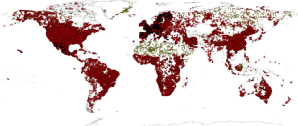
Also of great importance is how the data was processed. For making of the DSM only the data with less than 30% cloud coverage has been used, which approximately resulted in 3 million scenes. Figure 4.4 presents the number of overlapping scenes on a global map. On average number of stacked images for the globe is 4.62, and data covers 91.58% of Earth land area [63]. The areas least covered are Antarctica 48% and Greenland 38%.

A problem with altitude fluctuations of the satellite which sometimes caused jitter noises along track was reported by the study [61]. It has been mitigated significantly by using attitude data of the satellite sampled at much higher rate (10Hz PAD vs 675Hz HAD). For further processing the software package “DSM and Ortho-image Generation Software for ALOS PRISM (DOGS-AP)” was developed to streamline the calibration, processing and development of Digital Surface Models (DSMs) and Orthorectified Imagery (ORI) [60]. It does not need the Ground Control Points (GCPs) to achieve planimetric accuracy of 6.1m RMSE for nadir radiometer [59] [58], which presents value of calibration and detailed data preprocessing.

The results of papers confirm the high precision of the DSM, [57] shows that planimetric precision in plain condition can reach 2m RMSE, while on rougher terrain higher than 8m, [62] states precision in selected scenes reaching 1m RMSE compared to ICESAT data, and

(50)

32 Data overview

Figure 4.4 The status of PRISM stereo scenes in the archive with less than 30% cloud cover.[57]

high correlation with SRTM-3 data, though with larger RMSE deviations 1.93m-11.38m, which was explained by slight differences of instabilities of the orbits between Space shuttle and Satellite. GCPs have confirmed 3.94m RMSE on 122 points. One more detailed study was done in 2016 [63], which presents the analysis of the precision using global GCPs, and shows very good results, confirming previous studies, RMSE mostly better than 5m as can be seen on the Figure 4.5.

Such commercial high precision DSM has been resampled to 30m resolution using 7x7 pixel average value, and released to the public. The horizontal and vertical accuracy of the data is supposed to stay about the same, but in coarser resolution.

4.1.4 ISRIC SoilGRIDS

SoilGrids is the data set describing the soils on the global scale. It was released at first at 1km spatial resolution in December 2013, later at 250m in June 2016. SoilGrids250 database consists of global predictions for numeric soil properties (organic carbon, bulk density, Cation Exchange Capacity (CEC), pH, soil texture fractions and coarse fragments) at seven standard depths (0, 5, 15, 30, 60, 100 and 200 cm), predictions of depth to bedrock and distribution of soil classes based on the World Reference Base (WRB) and USDA classification systems

For training the prediction model around 110,000 for 1km and 150,000 soil profiles Figure 4.6 for 250m version and a stack of 158 remote sensing-based soil covariates (primarily derived from MODIS land products, SRTM DEM derivatives, climatic images and global landform and lithology maps) were used. Linear regression algorithms were used for SoilGrids1km version [28], after which it was found that other types of machine learning

(51)

Figure 4.5 Histogram of the height differences from 4,628 GCPs.[63]

Figure 4.6 Input profile data: World distribution of soil profiles used for model fitting (about 150,000 points shown on the map; see acknowledgments for a complete list of data sets used). Yellow points indicate pseudo-observations.[35]