TRACKING MEP INSTALLATION WORKS *F. Bosché
Heriot-Watt University, Edinburgh, EH14 4AS, UK
(*Corresponding author: [email protected])
Y. Turkan
Iowa State University, Ames, IA, USA
C.T. Haas
University of Waterloo, Waterloo, ON, Canada
T. Chiamone, G. Vassena and A. Ciribini
Università degli Studi di Brescia, Brescia, Italy
TRACKING MEP INSTALLATION WORKS ABSTRACT
Previous research has shown that “Scan-vs-BIM” systems are powerful to provide valuable information for tracking structural works (progress, quality, safety). However, the transferability of this capability to other construction areas such as MEP works has not been assessed so far. Comparatively, the construction of MEP systems, in particular pipes and ducts, tends to be more flexible with respect to the positioning of individual components, so that Scan-vs-BIM systems could be defeated when tracking MEP installation works. This paper presents recent results on the feasibility and performance of using a Scan-vs-BIM system to track MEP works. The approach followed is presented and then tested with two real-life challenging case studies were conducted simultaneously but totally independently in Canada and Italy. The results show that, as expected, pipes and ducts tend to be more loosely positioned than structural elements leading to a poorer performance of the Scan-vs-BIM system. Nonetheless, it appears that the system works well to assess the level of conformance of site installation works, providing valuable information for estimating emerging performance metrics like “percent built as-designed”. In addition, the proposed system could also be useful to accelerate and thus reduce the cost of delivering as-built BIM models for in the case of new builds.
KEYWORDS
Construction, MEP, Scan-vs-BIM, Laser Scanning, as-built status, percent built as designed INTRODUCTION
Progress Tracking in the AEC Industry
Monitoring progress has traditionally been an extensive manual operation that requires visual inspections be conducted by inspectors relying on personal judgment, and with a high probability of incomplete and inaccurate reports. In the early 2000’s, the Architectural-Engineering-Construction/Facility Management (AEC/FM) industry recognized the urgent need for quick and accurate project progress assessment; the way of monitoring progress had to be reinvented and automated.
In order to address this situation, researchers have suggested using different types of new technologies for automating, at least partially, the inspection and assessment process. Investigated technologies mainly include Radio Frequency Identification (RFID) (Grau, 2009; Ergen, 2007; Li, 2011; Pradhan, 2009; Razavi, 2010; Razavi, 2012), Ultra-Wide Band (UWB) (Teizer, 2008; Cheng, 2011; Shahi, 2012; Saidi, 2011), Global Positioning System (GPS) (Grau, 2009), Photogrammetry (Golparvar-Fard, 2009; Golparvar-Fard, 2013), and Three-dimensional Terrestrial Laser Scanning (TLS) (Bosché and Haas, 2008; Kim, 2013; Stone, 2001; Tang, 2010; Tang, 2011).
All these approaches hold much promise for automated progress tracking, but they have so far only focused on a few areas of application: progress in the supply chain (prefabrication and laydown yards), workers’ productivity (through location and action tracking), and tracking structural work progress. One of the important areas where tracking could provide significant value but that has not been investigated so far is Mechanical, Electrical and Plumbing (MEP) installation works: HVAC, piping installation, etc. The benefits of efficient tracking of MEP installation works include:
• Early identification of deviations between the as-built and as-design situations, so that remedying actions can be taken before high rework costs are experienced.
• Faster acceptation of work by the main contractor, so that sub-contractors can be paid on time and even earlier than common practice (an important issue with regard to the sustainability of the industry). Three dimensional (3D) Terrestrial Laser Scanning (TLS), also called LADAR (Laser Detection and Ranging), has been considered by many as the best available technology to capture 3D information on a project with accuracy and speed, with a wide range of applications in the AEC/FM industry (Stone, 2001; Tang, 2011; Jacob, 2008). Laser scanning has been proven to be valuable for construction managers to help them for many tasks such as progress monitoring, quality control and facility/infrastructure management (Biddiscombe, 2005; Bosché, 2008; Lee, 2012; Lijing, 2008; Park, 2007; Qui, 2008; Valero, 2013; Xiong, 2013; Yen, 2008). All these works illustrate the large range of applications of laser scanning technology today, and explain why the market for laser scanning hardware and software has grown exponentially in the last decade. Much of this growth is now focusing on the interface between scanned data and Building Information Models (BIMs).
Scan-to-BIM and Scan-vs-BIM
One of the main applications of laser scanning today remains what is commonly called
Scan-to-BIM, which aims to reconstruct as-built 3D BIM models from the acquired 3D point clouds. But, the rapid development of 3D modeling and BIM offers other perspectives: in the case of new builds, by aligning TLS scans of construction sites with project 3D BIM models, control of progress and dimensional quality can be significantly improved in terms of scope, accuracy and speed. We call this approach: Scan-vs-BIM.
Recent work has shown that object-based recognition techniques based on Scan-vs-BIM frameworks indeed enable the recognition of 3D BIM objects in TLS data for supporting progress and dimensional quality control (Bosché, 2008; Bosché, 2009; Kim, 2013; Tang, 2011; Turkan, 2011; Turkan, 2013). Similar approaches are also investigated using 3D point clouds generated through photogrammetry instead of TLS (Golparvar-Fard, 2009; Golparvar-Fard, 2013).
Contribution
While the potential of Scan-vs-BIM frameworks has already been demonstrated for structural work control, no research results have yet been reported on whether such approach actually works for other areas of construction, in particular MEP installation works. Such investigation is necessary because, contrary to structural works, the installation of MEP systems in practice is much more flexible with respect to the locations of the individual elements and routes.
This paper presents experiment results on the assessment of the effectiveness of a Scan-vs-BIM framework to control MEP works through real-life case studies. Two sets of experiments are reported. They both used the Scan-vs-BIM system developed by Bosché et al. (2008; 2009), but were conducted totally independently from one another in Canada and Italy. It is thus expected that the results obtained give reliable insight the overall aim of the research.
THE APPROACH
In this section, we summarize the Scan-vs-BIM object recognition system proposed by Bosché et al. (2008; 2009) and how it is used to recognize progress of MEP pipe and duct installation activities. Registration
The first (and most critical) step of the Scan-vs-BIM approach consists in aligning the 3D point clouds in the same coordinate system as the 3D model; this is commonly called registration. This should normally be performed using site benchmarks. If structural works have been successfully controlled, it is also possible to use the building structure as natural landmarks for the registration, e.g using the plane-based registration approach presented in (Bosché, 2011).
Once registration is completed for all available scans, as-built objects can be recognized in the combined point cloud. The recognition algorithm has four steps:
1 – Matching/Recognized Point Clouds: For each scan, each point is matched with a 3D model object. Matching is done by projecting the point orthogonally on the surfaces of all NObj objects of the 3D BIM model. The closest surface is identified, and if the distance to that surface, δ, is lower than a threshold δmax, and the difference between the point and object surface normal vectors, α, is lower than a threshold αmax, then the point is considered matched to the corresponding object. The result of this process is a segmentation of each initial scan into NObj+1 point clouds; one per object that includes all the points matched to that object as well as a one containing all the points not matched to any model object. We call the latter the “NonModel” point cloud.
2 - Occluding Point Clouds: For each as-built scan, the NonModel point cloud is further processed to identify the NonModel points that lay between the scanner and 3D model objects. The result of this process is not just an overall occlusion point cloud, but also its segmentation into NObj point clouds; one per object that includes all the points occluding that object.
3 - As-planned Point Clouds: For each scan, a corresponding virtual as-planned scan is calculated. This is done using the 3D model and the same scanner’s location and scan resolution as one of the actual (as-built) scan obtained from the registration process. Each as-planned point is calculated by projecting a ray from the scanner onto the 3D model. The result of this process is not just an as-planned scan, but also its segmentation into NObj point clouds; one per object that includes all the points matched to that object. Note that we do not retain any NonModel as-planned point cloud.
4 - Object Recognition: The results of the first three steps are finally aggregated. Each model object then has:
• A matched (or recognized) point cloud containing all the scanned points matched to that object.
• An occlusion point cloud containing all the points occluding that object.
• An as-planned point cloud containing all the as-planned points matched to that object. We then convert these point clouds into corresponding surface areas by adding up the surfaces covered by each point in each point cloud – for details, see (Bosché, 2009). The result is for each model object:
• A matched/recognized surface area, Srecognized. • An occlusion surface area, Soccluded.
• An as-planned surface area, Splanned.
These surface areas allow the calculation of different metrics regarding the recognisability (occlusion) and recognition of each object, namely:
%recognized = Srecognized / Srecognizable = Srecognized / (Splanned-Soccluded) %confidence = Swrecognized / Srecognizable = Swrecognized / (Splanned-Soccluded)
with Swrecognized=∑iϵ[1;n](1-|δi/δmax| 2
)Si
Swrecognized is a weighted recognized surface where the contribution of each point to the recognized
surface is weighted based on the quality of its matching (distance).
We use Srecognized and %recognized to infer the recognition of each object using the following rule: If ((Srecognized≥Smin) or (%recognized>%rmin)), then the object is considered recognized. We typically define Smin=500cm2 and %rmin=50%. This rule enables the recognition of both large and small (i.e. for which Srecognizable<Smin). Furthermore, the values are chosen large enough to ensure that objects are recognized only if there is sufficient support from the point clouds.
Finally, %confidence extends %recognized by taking account for the deviation between the as-built and designed positioned of objects, and can be as a measure of the level of recognition in the recognition of each object.
EXPERIMENTS
Experiments have been conducted using real life case studies to evaluate the performance of the proposed approach. Two different sets of experiments were conducted in parallel but entirely independently from one another: one in Canada, the other in Italy. The results obtained for each of them are presented below. Section 4 will then discuss the overall outcome of the experiments.
Canadian Experiment
The project for which data was acquired is the Engineering VI Building at the University of Waterloo, a five-storey, 100,000-square-foot building that is designed to shelter the Chemical Engineering Department of the university. The attention of this study was focused on the 31.0m x 3.4m service corridor of the 5th floor of the building because of the abundance of pipes coming from the lower levels and going all the way up to the penthouse.
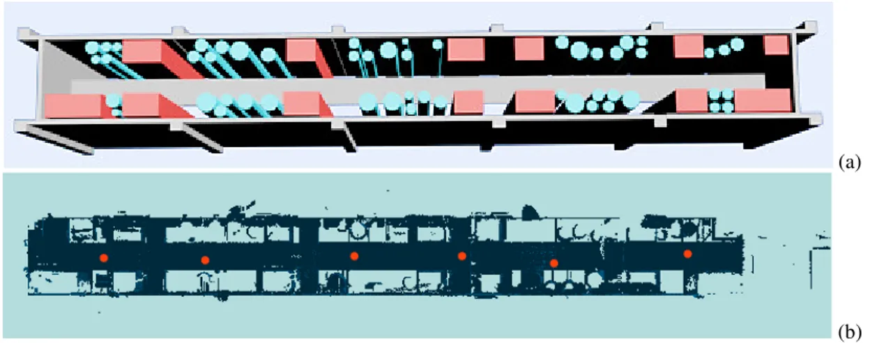
The data collected includes: (1) 2D CAD drawings from that the authors followed to create a 3D model (Figure 1a); (2) a set of six TLS scans acquired on February 5th 2011 with a FARO Laser Scanner LS 880 HE [37] and covering the entire length of the corridor (Figure 1b). Each scan contains about 1,000,000 points.
(a)
(b) Figure 1: The 3D model (a) and 6 scans (b) for the 5th floor service corridor of the E6 Building.
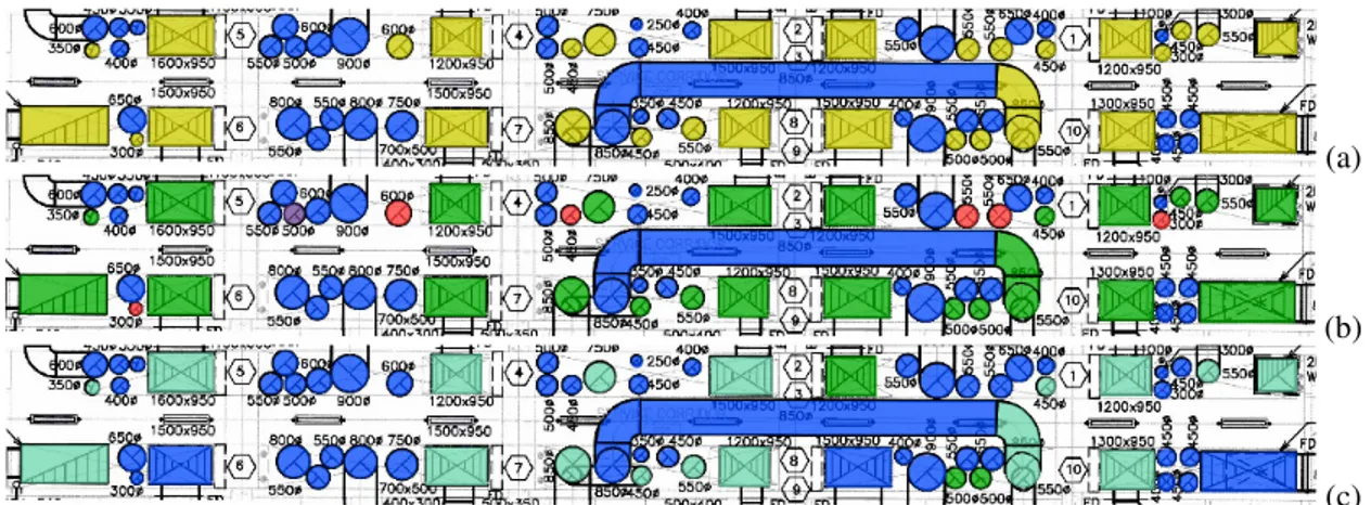
Figure 2(a) shows the result of a manual analysis of the combined point cloud to identify the actual presence of the different mechanical objects. This information is used solely as ground truth for the calculation of its performance detailed below.
Figure 2(b) then illustrates the object recognition results for δmax=30mm and Smin=500cm 2 (additional experiments not reported here have shown that this value of δmax, the most critical of the two parameters, is most appropriate). It highlights which objects are correctly recognized (true positive; TP), incorrectly recognized (false positive; FP), correctly not recognized (true negative; TN) and incorrectly not recognized (false negative; FN). Table 1 summarizes the results of Figure 2, and leads to a Recall rate of 81% and a Precision rate of 96%.
Figure 2(c) details the level of confidence reported by the software for all correctly recognized objects (TP). In this figure, objects are colored based on %recognized and grouped in four categories of level of confidence: High (50%<%recognized); Medium-low (5%<%recognized<50%); Very low (%recognized<5%). These categories were defined ad-hoc and were found to be quite representative of the different situations encountered.
(a)
(b)
(c) Figure 2: Experiment results for the Canadian experiment:
(a) Manual analysis of the presence of mechanical elements in the point cloud: Yellow: element present; Blue: element absent.
(b) Mechanical elements recognition result for δmax = 30mm and Smin = 500cm2: Green: true positive; Red: false negative; Blue: true negative; Magenta: false positive.
(c) Level of confidence, based on %recognized, for all the recognized elements: Green: high level of conference (50%<%recognized); Turquoise: medium-low level of confidence (5%<%recognized<50%) ; Blue:
very low level of confidence (%recognized<5%).
Table 1 – Object recognition results for the Canadian experiment. As-built state Recognized state Present Absent Present 26 6 Absent 1 39
The high precision rate above illustrates the robustness of the system with regard to false positives. This is mainly explained by the combination of the distance and normal vector criteria in the point matching procedure that increase the likelihood that points are correctly matched. For a false positive to occur, an object would need to be located in a way that its surface is aligned with the designed surface of another object. While this still occurs once in this experiment, it can be noted that the confidence level reported by the system for that object is actually very low. This suggests that the confidence level can play an important role in avoiding false positives, and could even be used as an additional criterion in the recognition rule.
The recall rate, while not very low, is disappointing particularly when compared with performances obtained in previous research on tracking structural work, where recall (and precision) achieved nearly 100% (Bosché, 2009; Turkan, 2011). Furthermore, the level of confidence reported for the correctly recognized objects is generally quite low (< 50% for most objects), which is also poor in comparison with results obtained for structural elements. These results are explained by the fact that, as was anticipated, installation of mechanical elements is geometrically less constrained than that of structural elements, so that the actual and designed poses of some mechanical elements may differ. Two of the false negatives are illustrated in Figure 3(c) below.
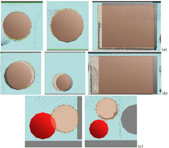
Despite these disappointing recall results, it is worth noting that there appears to be a good correlation between the actual level of deviation between the as-built and designed poses of objects and the reported levels of confidence, %confidence (see examples in Figure 3). The value of this observation is discussed further in Section Discussion and Conclusion.
(a)
(b)
(c)
Figure 3: Correlation between level of confidence, %confidence, and deviation between built and as-planned poses of elements. The actual pose of each element (in the point cloud) is highlighted in transparent orange. Top row: Elements recognized with high level of confidence; Middle row: Elements recognized with medium-low level of confidence; Bottom row: Elements not recognized (false negatives). Italian Experiment
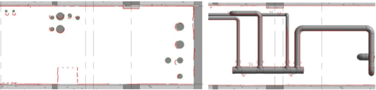
A great Hospital located in the North of Italy is the construction site object of the study. The main block extends over an area of 35,000 square meters and includes the whole construction of four buildings and the complete restoration of a fifth. The collected data includes first of all 2D drawings, from which the structure has been translated into a 3D BIM model. The structures are modeled using Autodesk® Revit® Structure, whereas some parts of the plant facilities (pipeline and ducts) are modeled using Autodesk® Revit® MEP. The survey campaign was performed on May and June 2012 using a Faro Focus 3D Laser Scanner. Each scan is acquired with a 1/8 resolution ratio and contains about 1,000,000 points. This resolution is chosen in order to reduce the period of data recording (about 2'30") and the interference with construction site works. The survey area chosen for this study covers the 2nd basement of the building under construction, because of a large number of air conditioning ducts and plumbing laid on them (Figure 4). Four scans of the basement were acquired and used for the experiment.
Figure 4: The 3D model (left) and the scans (right) for the service area in the 2nd basement.
Figure 5 illustrates the object recognition results. It draws attention to which objects are correctly recognized (green) and incorrectly not recognized (red). The parameters used in the object recognition analysis are δmax=30mm, Smin=300cm2 and %min=50% (the chosen value for Smin is slightly smaller than for the Canadian experiment because of the smaller sizes of the pipes). Table 2 sums up the object recognition results, which lead to a recall rate of 32% and precision rate of 100%. Note that these results consider pipes, elbows and valves.
(a) (b)
Figure 5: Object recognition (a) and level of confidence (b) for the Italian experiment. Table 2 – Object recognition results for the Italian experiment.
As-built State Recognized state Present Absent Present 73 152 Absent 0 1
These results lead to a similar conclusion to that obtained with the Canadian experiment. First of all, the perfect precision rate further demonstrates the robustness of the system with regard to false positives. However, the recall rate is even worse than for the Canadian experiment and is explained by two things: (1) as for the Canadian experiment, the flexibility in MEP installation works has led to situations where pipes are too far from their expected pose for the system to recognize them; the impact of this made worse here due to the smaller sizes of the pipes; (2) the combination of the small number of scans acquired, the density of pipes and their small sizes lead to significant occlusions and very small recognizable surfaces for a number of pipes. With more scans acquired at critical locations, the authors estimate that the recall could have increased to around 60%.
In addition, the Italian experiment confirms that the level of confidence %confidence is often low, even for correctly recognized objects (see Figure 5(b)). However, the same observation is made that the
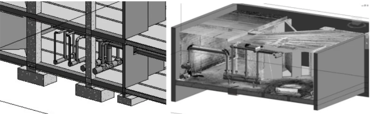
automatically calculated confidence level appears to be a good indicator of the amount of deviations between the as-built and designed pose of objects. Figure 6 illustrates deviations typically observed between the scans’ point clouds and the project 3D model.
Figure 6: Two vertical cross-sections visualizing the comparison between the scanned data and 3D model for the 2nd basement.
DISCUSSION AND CONCLUSION
Two parallel and independent experiments have been conducted to assess the performance of a Scan-vs-BIM framework to track MEP works on construction projects. The results are generally disappointing and are explained by the geometrical flexibility typically given to MEP installation work. As a result, it is anticipated that automatically tracking MEP works using TLS data should be achieved by combining a Scan-vs-BIM approach with more active object recognition techniques based on geometry (e.g. cylinder, planes) and appearance (material) recognition algorithms.
Nonetheless, the high precision rates and the fact that the level of confidence appears to be a good indicator of the amount of deviations between the as-built and designed poses of objects suggest that the proposed approach could be useful for two other valuable applications:
• “Percent built as designed”: “Percent built as designed” is a performance criterion emerging in practice. In essence it aims at estimating quality performance, by quantifying the overall deviation between the designed and as-built state of projects. The proposed could enable the automated estimation of such performance criterion, with focus on geometry/dimensions.
• Delivery of true as-built BIM model: Operation & Maintenance (O&M) managers tend not to trust old or recent drawings (including BIM models) produced by the design team because of discrepancies with the actually built facilities. In order to have BIM models usable for O&M, scan-to-BIM procedures are employed to produce accurate models. However, the authors argue that, while existing drawings may not be perfect, experiments show that they are generally not entirely wrong. Integrating the proposed Scan-vs-BIM system within as-built modelling frameworks would enable modellers to rapidly identify which objects are built as designed and thus don’t need to be remodelled. By focusing only on those elements that deviate or are missing from design models, a significant amount of modelling time and cost could be saved.
Future work will focus on experimentally assessing the value of the proposed Scan-vs-BIM framework for the two applications above. Furthermore, it is worth noting the Canadian and Italian experiments used MEP works for which little pre-fabrication was used, which explains the observed deviations. For project using off-site pre-fabrication and sub-assembly, it is expected that smaller deviations be observed, in which the proposed approach may demonstrate much higher performance. Corresponding data will be acquired to investigate whether such improved performance is indeed achieved.
REFERENCES
Biddiscombe, P. (2005). 3D Laser scan tunnel inspections keep expressway infrastructure project on
Bosché, F., Haas, C.T. (2008). Automated retrieval of 3D CAD model objects in construction range images,
Automation in Construction, 17, pp. 499-512.
Bosché, F. (2009). Automated recognition of 3D CAD model objects and calculation of as-built dimensions for dimensional compliance control in construction, Advanced Engineering
Informatics, 24, pp. 107-118.
Bosché, F. (2011). Plane-based Coarse Registration of 3D Laser Scans with 4D Models, Advanced Engineering Informatics, 26, pp. 90-102.
Cheng, T., Venugopal, M., Teizer, J., Vela, P.A. (2011). Performance evaluation of ultra-wideband technology for construction resource location tracking in harsh environments, Automation in
Construction, 20, pp.1173-1184.
Ergen, E., Akinci, B., Sacks, R. (2007). Life-cycle data management of engineered-to-order components using radio frequency identification, Automation in Construction, 21, pp. 356-366.
Golparvar-Fard, M., Pena-Mora, F., Savarese, S. (2009). Application of D4AR – A 4-Dimensional augmented reality model for automating construction progress monitoring data collection, processing and communication, Journal of Information Technology in Construction, 14, pp. 129-153.
Golparvar-Fard, M., Peña-Mora, F., Savarese, S. (2013). Automated progress monitoring using unordered daily construction photographs and IFC-based Building Information Models, ASCE Journal of
Computing in Civil Engineering, in press.
Grau, D., Caldas, C. H., Haas, C. T., Goodrum, P. M., Gong, J. (2009). Assessing the impact of materials tracking technologies on construction craft productivity, Automation in Construction, 18, pp. 903-911.
Jacobs G. (2008). 3D scanning: Using multiple laser scanners on projects, Professional Surveyor Magazine, 28.
Kim, C., Son, H., Kim, C. (2013). Automated construction progress measurement using a 4D building information model and 3D data, Automation in Construction, 31, pp. 75-82.
Lee, J., Kim, C., Son, H., Kim, C.-H. (2012). Automated pipeline extraction for modeling from laser scanned data, International Symposium on Automation and Robotics in Construction (ISARC), Eindhoven, the Netherlands.
Li, N., Becerik-Gerber, B. (2011). Performance-based evaluation of RFID-based Indoor Location Sensing Solutions for the Built Environment, Journal of Advanced Engineering Informatics, 25 (3), pp. 535–546.
Lijing, B., Zhengpeng, Z. (2008). Application of point clouds from terrestrial 3D laser scanner for deformation measurements, The International Archives of the Photogrammetry, Remote Sensing
and Spatial Information Sciences, 37.
Park, H.S., Lee, H.M., Adeli, H., Lee, I. (2007). A new approach for health monitoring of structures: terrestrial laser scanning, Journal of Computer Aided Civil and Infrastructure Engineering, 22, pp.19-30.
Pradhan, A., Ergen, E., Akinci, B. (2009). Technological Assessment of Radio Frequency Identification Technology for Indoor Localization, ASCE Journal of Computing in Civil Engineering, 23 (4), pp. 230-238.
Qui, D. W., Wu, J. G. (2008). Terrestrial laser scanning for deformation monitoring of the thermal pipeline traversed subway tunnel engineering, XXIst ISPRS Congress: Commission V, WG 3, Beijing, pp. 491-494.
Razavi, S. N., Haas, C. T., (2010). Multisensor data fusion for on-site materials tracking in construction,
Automation in Construction, 19, pp. 1037-1046.
Razavi, S.N., Moselhi, O. (2012). GPS-less indoor construction location sensing, Automation in
Construction, 28, pp. 128-136.
Saidi, K. S., Teizer, J., Franaszek, M., Lytle, A. M. (2011). Static and dynamic performance evaluation of a commercially-available ultra wideband tracking system, Automation in Construction, 20, pp. 519-530.
Shahi, A., Aryan, A., West, J. S., Haas, C. T., Haas, R. G. (2012). Deterioration of UWB positioning during construction, Automation in Construction, 24, pp. 72-80.
Stone, W., Cheok, G. (2001). LADAR sensing applications for construction, Building and Fire Research, National Institute of Standards and Technology (NIST), Gaithersburg, MD.
Tang, P., Huber, D., Akinci, B., Lipman, R., Lytle, A. (2010). Automatic reconstruction of as-built building information models from laser-scanned point clouds: A review of related techniques,
Automation in Construction, 19(7), pp. 829-843.
Tang, P., Anil, E., Akinci, B., Huber D. (2011). Efficient and Effective Quality Assessment of As-Is Building Information Models and 3D Laser-Scanned Data, ASCE International Workshop on
Computing in Civil Engineering, Miami, FL, USA.
Teizer, J., Venugopal, M., Walia, A. (2008). Ultrawideband for Automated Real-time Three-Dimensional Location Sensing for Workforce, Equipment, and Material Positioning and Tracking,
Transportation Research Record, Transportation Research Board of the National Academies, Washington D.C, pp. 56–64.
Turkan, Y., Bosché, F., Haas, C. T., Haas, R. G. (2011). Automated progress tracking using 4D schedule and 3D sensing technologies, Automation in Construction, 22, pp. 414-421.
Turkan, Y., Bosché, F., Haas, C.T., Haas, R. (2013). Automated Earned Value Tracking using 3D Imaging Tools, ASCE Journal of Construction Engineering and Management, in press.
Valero, E.,Adán, A. and Cerrada, C. (2012). Automatic method for building indoor boundary models from dense point clouds collected by laser scanners, Sensors, 12, pp. 16099-16115.
Xiong, X., Adán, A., Akinci, B., Huber, D. (2013). Automatic creation of semantically rich 3D building models from laser scanner data, Automation in Construction, 31, pp. 325-337.
Yen, K.S, Akin, K., Ravani, B. (2008). Accelerated Project Delivery: Case Studies and Field Use of 3D
Terrestrial Laser Scanning in Caltrans Projects, Advanced Highway Maintenance and Construction Technology Research Center, Research Report UCD-ARR-08-06-30-0.