DIENCA - UNIVERSITY OF BOLOGNA Via dei Colli 16, 40136 Bologna, Italy
TECHNICAL REPORT LIN-THRG 108:
A THREE-DIMENSIONAL CFD PROGRAM FOR THE SIMULATION OF THE THERMO-HYDRAULIC BEHAVIOUR OF AN OPEN CORE LIQUID METAL
REACTOR Dec 16 2008
Authors: A.Cervone and S.Manservisi [email protected] [email protected]
Abstract. A thermo-fluid dynamics code with the purpose to investigate three-dimensional pressure, velocity and temperature fields inside nuclear reactors is presented in this work. The code computes pressure,velocity and temperature fields at the coarse fuel assembly level when all the sub-channel de-tails are summarized in parametric coefficients. A 3D CFD model for an open core liquid metal reactor has been implemented on a finite element code and some preliminary tests for generic geometries are reported.
1 Introduction 2
1.1 Finite element model . . . 3
1.1.1 Navier-Stokes system. . . 3
1.1.2 Variational form of the Navier-Stokes equations . . . 3
1.1.3 Finite element Navier-stokes system . . . 4
1.1.4 Two-level finite element Navier-Stokes system . . . 5
1.2 Reactor model. . . 9
1.2.1 Reactor geometry and mesh generation . . . 9
1.2.2 Reactor transfer Operators in working conditions . . . 9
1.2.3 Reactor Equations in working conditions . . . 12
1.2.4 Thermophysical properties of liquid metals (lead) . . . 13
2 CFD Program 15 2.1 Introduction . . . 15
2.1.1 Installation . . . 15
2.1.2 Preprocessor and mesh generation . . . 15
2.1.3 Running the code . . . 15
2.1.4 Postprocessing . . . 16
2.2 Directory structure . . . 17
2.2.1 Generalities . . . 17
2.2.2 Main directory and C++ classes. . . 17
2.2.3 Directory config . . . 18
2.2.4 Directory contrib . . . 18
2.2.5 Directory data_in . . . 18
2.2.7 Directory output . . . 19
2.3 Configuration, data and parameter setting . . . 20
2.3.1 Configuration . . . 20
2.3.2 Data . . . 22
2.3.3 Boundary conditions . . . 25
2.3.4 Initial conditions . . . 26
2.3.5 Physical property dependence on temperature . . . 26
2.3.6 Power distribution and pressure loss distribution . . . 27
3 Tests 30 3.1 Monodimensional test (test1) . . . 30
3.1.1 Monodimensional equations . . . 30
3.1.2 Monodimensional analytic test . . . 30
3.1.3 Simulations with constant axial power distribution (test1). . . 32
3.2 Simulations of a test reactor model . . . 34
3.2.1 Reactor model core . . . 34
3.2.2 Test without control rod assemblies (test2) . . . 36
3.2.3 Test with control rod assemblies (test3) . . . 40
3.2.4 Test with intra-assembly turbulent viscosity (test4) . . . 46
A Code documentation 50 A.1 Class index . . . 50
A.1.1 Reactor model (RM) code File List . . . 50
A.2 Class documentation . . . 50
A.2.1 MGCase Class Reference . . . 50
A.2.1.1 Member Data Documentation . . . 51
A.2.2 MGGauss Class Reference . . . 52
A.2.3 MGMesh Class Reference . . . 53
A.2.4 MGSol Class Reference . . . 55
A.2.5 MGSolT Class Reference . . . 58
A.3 Reactor Model code File documentation . . . 61
A.3.1 The main file ex13.C . . . 61
A.3.2 Configuration file config.h . . . 66
Introduction
A full 3D CFD code with the purpose of analyzing the thermal hydraulic behaviour of an open core liquid metal reactor has been developed. The purpose of this code is to investigate three-dimensional pressure, velocity and temperature fields inside nuclear reactors at the coarse fuel assembly level when all the sub-channel details are summarized in parametric coefficients. The solution of the Navier-Stokes system and the energy equation is obtained by using the finite element method. This report consists of three Chapters and one Appendix: Chapter1introduces the mathematical model, Chapter
2describes the CFD code, Chapter3evaluates the code performance for some reactor configurations and AppendixAcan be used for class references.
In Section1.1, the full three-dimensional incompressible Navier-Stokes and energy equations are in-troduced. The numerical simulations take place at a coarse, assembly length level and are linked to the fine, sub-channel level state through transfer operators based on parametric coefficients that sum-marize local fluctuations. The overall effects between assembly flows are evaluated by using average assembly turbulent viscosity and energy exchange coefficients. In Section1.2 the computational re-actor model is described: the computational mesh, the rere-actor transfer operators for the rere-actor in working conditions and the lead thermophysical properties are defined.
The CFD code structure and the main commands are illustrated in different sections of Chapter2: the code installation, the preprocessing, the run and the postprocessing of the code results can be found in Section2.1. In Section2.2the code directory structure is illustrated. The Section2.3is dedicated to the configuration and data files. This section explains how to set the initial and boundary conditions and power and pressure loss coefficients.
In Section 3.1 some basic tests are performed for an open core geometry in order to compare this three-dimensional approach with the standard mono-dimensional one. The final section of Chapter
3describes different simulations for two geometries: the first geometry does not include the control rod area which is included in the other geometry. This code has been used, under the assumption of weakly correlated assemblies, for a preliminary assessment of an open square lattice with three fuel radial zones at different levels of enrichment.
The program described in this report is a class object oriented code and the appendix briefly presents these classes to help the interested reader to quickly modify part of the program. More details and more extensive information can be found in the html/tex/xml code documentation.
1.1 Finite element model
1.1.1 Navier-Stokes systemLet Ω be the domain and Γ be the boundary of the system. We assume that the state of this system is defined by velocity, pressure and temperature field (v, p, T ) and that its evolution is described by the solution of the following system
∂ρ ∂t + ∇ · (ρ v) = 0 , (1.1) ∂ρ v ∂t + ∇ · (ρvv) = −∇p + ∇ · ¯τ + ρg , (1.2) ∂ρ CpT ∂t + ∇ · (ρvCpT ) = Φ + ∇ · (k∇T ) + ˙Q , (1.3) where we can easily recognize the Navier-Stokes and energy equations. For our purposes the system can be considered incompressible, while the density is assumed only to be slightly variable as a function of the temperature, with ρ = ρ(T ) given. The tensor ¯τ is defined by
¯
τ = 2µ ¯D(u) , Dij(u) = 12(∂u∂xi j +
∂uj
∂xi) (1.4)
with i, j = x, y, z. In a similar way the tensor vv is defined as vvij = vivj. The quantity g denotes the gravity acceleration vector, Cp is the pressure specific heat and k the heat conductivity. ˙Q is the volume heat source and Φ the dissipative heat term.
1.1.2 Variational form of the Navier-Stokes equations
Now we consider the variational form of the Navier-Stokes system. In the rest of the paper we denote the spaces of all possible solutions in pressure, velocity and temperature with P (Ω), V(Ω) and H(Ω) respectively.
a) Incompressibility constraint. By multiplying the (1.1) by a scalar test function ψ in the space P (Ω) and integrating over the domain Ω we have the following variational form of the incompress-ibility constraint
Z
Ω ψ
∂ρ
∂t + ψ ∇ · (ρ v) dx = 0 ∀ψ ∈ P (Ω) . (1.5) b) Momentum equation. If one multiplies (1.2) for the three-dimensional test vector-function φ in the space V(Ω) and integrates over the domain Ω one has, after integration by parts, the following variational momentum equation
Z Ω ∂ ρ v ∂t · φ dx + Z Ω(∇ · ρvv) · φ dx = Z Ω p ∇ · φ dx − Z Ω τ : ∇φ dx +¯ Z Ω ρg · φ dx − ∀φ ∈ V(Ω) (1.6) Z Γ(p~n − ¯τ · ~n) · φ ds .
The surface integrals must be computed by using the boundary conditions and they are zero if appropriate boundary conditions are imposed. We remark that if we set φ = δv where δv is a variation of the velocity field v then (1.6) is the equation for the evolution of the rate of the virtual work.
c) Energy equation. Finally for the energy equation, if we multiply for the scalar test function ϕ in the space H(Ω) and integrate over the domain Ω we have, after integration by parts, the following variational energy equation
Z Ω ∂ ρ CpT ∂t ϕ dx + Z Ω ∇ · (ρ vCpT ) ϕ dx = Z Ω Φ ϕ dx − Z Ω k ∇T · ∇ϕ dx + Z Ω ˙ Qϕ dx + ∀ϕ ∈ H(Ω) (1.7) Z Γ(k∇T · ~n) ϕ ds .
Again, the surface term must be computed by imposing the appropriate boundary conditions. 1.1.3 Finite element Navier-stokes system
The pressure space P (Ω), the velocity space V(Ω) and the energy space H(Ω) in (1.5-1.7) are in general infinite dimensional spaces. If the spaces P (Ω), V(Ω) and H(Ω) are finite dimensional then the solution (v, p, T ) will be denoted by (vh, ph, Th) and the corresponding spaces by Ph(Ω), Vh(Ω) and Hh(Ω). In order to solve the pressure,velocity and energy fields we use the finite space of linear polynomials for Ph(Ω) and the finite space of quadratic polynomials for Vh(Ω) and Hh(Ω). In this report the domain Ω is discretized always by Lagrangian finite element families with parameter h. The finite element Navier-Stokes system becomes
a) Fem incompressibility constraint Z
Ω ψh
∂ρ
∂t + ψh∇ · (ρ vh) dx = 0 ∀ψh∈ Ph(Ω) , (1.8) b) Fem momentum equation
Z Ω ∂ ρ vh ∂t · φhdx + Z Ω(∇ · ρ vhvh) · φhdx = Z Ω ph∇ · φhdx − Z Ω τ¯h: ∇φhdx + Z Ω ρg · φhdx − ∀φh ∈ Vh(Ω) (1.9) Z Γ(ph~n − ¯τh· ~n) · φhds ,
c) Fem energy equation Z Ω ∂ρ CpTh ∂t ϕhdx + Z Ω ∇ · (ρvhCpTh) ϕhdx = ∀ϕh∈ Hh(Ω) (1.10) Z Ω Φhϕhdx − Z Ω k ∇Th· ∇ϕhdx + Z Ω ˙ Qhϕhdx + Z Γ k ∇Th· ~n ϕhdx .
Since the solution spaces are finite dimensional we can consider the basis functions {ψh(i)}i, {φh(i)}i and {ϕh(i)}i for Ph(Ω), Vh(Ω) and Hh(Ω) respectively. Therefore the finite element problem (1.8
-1.10) yields a system of equations which has one equation for each fem basis element. 1.1.4 Two-level finite element Navier-Stokes system
Let us consider a two level solution scheme where a fine level and a coarse level solution can be defined. At the fine level the fluid motion is exactly resolved by the pressure, velocity and temperature solution fields. We denote by {ψh(i)}i, {φh(i)}iand {ϕh(i)}i the basis functions for Ph(Ω), Vh(Ω) and Hh(Ω). Different from the fine level is the coarse level which takes into account only large geometrical structures and solves only for average fields. The equations for these average fields (coarse level) should take into account the fine level by using information from the finer grid through level transfer operators. The definition of these transfer operators is still an open problem. We use the hat label for all the quantities at the coarse level. In particular we denote the solution at the coarse level by (ˆph,vbh, ˆTh) and the solution spaces byPbh(Ω),Vbh(Ω) andHbh(Ω) respectively.
Momentum equation. Let (ph, vh) ∈ Ph(Ω) × Vh(Ω) be the solution of the problem at the fine level obtained by solving the equation
Z Ω N S(ph, vh) · φh(i) dx = 0 , (1.11) or Z Ω ∂ ρ vh ∂t · φh(i) dx + Z Ω(∇ · ρ vhvh) · φh(i) dx − Z ΓZ(¯τh· ~n − ph~n) · φh(i) ds − (1.12) Ω ph∇ · φh(i) dx + Z Ω τ¯h : ∇φh(i) dx − Z Ω ρg · φh(i) dx = 0
for all the elements of the basis {φh(i)}i in Vh(Ω). The test function φhmust have a small compact support necessary to describe all the channel details and satisfy all the boundary conditions. Now consider the solution (ˆph,vbh) at the coarse level (fuel assembly level). It is clear that (ˆph,vbh) is different from (ph, vh) and should satisfy the Navier-Stokes equation with test functions φbh large enough to describe only the assembly details and satisfy the boundary conditions at the coarse level. Therefore if we substitute the coarse solution (ˆph,vbh) in (1.12) we have
Z Ω ∂ ρvbh ∂t · φh(i) dx + Z Ω(∇ · ρ b vhvbh) · φh(i) dx + Z ΓZ(pbh~n − ¯τbh· ~n) · φh(i) ds − (1.13) Ω pbh∇ · φh(i) dx + Z Ω ¯ b τh: ∇φh(i) dx − Z Ω ρg · φh(i) dx = Z Ω P m cf(pbh− ph,bvh− vh) · φh(i) dx + Z Ω T m cf(vh,vbh) · φh(i) dx , where the momentum fine-coarse transfer operator Pm
cf(bph− ph,vbh− vh) is defined by
and the turbulent transfer operator Tm
cf(vh,vbh) by
Tcfm(vh,vbh) = −∇ · ρ vhvh+ ∇ · ρvbhvbh− ∇ · ρ (vbh− vh)(bvh− vh) . (1.15) The momentum fine-coarse transfer operator Pcf(ph−pbh, vh −bvh) defines the difference between the rate of virtual work in the fine and in the coarse scale. The turbulent transfer operator Tm
cf(vh,vbh) gives the turbulent contribution from the fine to the coarse level.
Since the coarse scale is defined by a set of solutions inPbh(Ω),Vbh(Ω) we must write the equation (1.15) with the test functions (ψbh,φbh) inPbh(Ω) ×Vbh. We assume that the finite element space on the fine and coarse grid are embedded, namelyPbh(Ω) ⊂ Ph(Ω) andVbh(Ω) ⊂ Vh(Ω). This implies that
b
φh ∈ Vbh(Ω) can be computed as a linear combination of functions in Vh(Ω). Since these are finite dimensional spaces we have
b φh(k) = Nk X i=1 ai(k)φh(i) . (1.16)
For finite element spaces constructed with Lagrangian polynomials, the coefficients ai(k) are b
φh(xi)(k) where xi is a vertex point associated with the basis function φbhi at the fine level. If we multiply the (1.12) by ai(k) and add all the equations inφbhi over the Nk basis functions, after straightforward computations, we have
Z Ω ∂ ρvbh ∂t · Nk X i=1 ai(k)φh(i) dx + Z Ω(∇ · ρvbhvbh) · Nk X i=1 ai(k)φh(i) dx + Z Γ(pbh~n − ¯τbh· ~n) · Nk X i=1 ai(k)φh(i) ds − (1.17) Z Ω b ph∇ · Nk X i=1 ai(k)φh(i) dx + Z Ω ¯ b τh : ∇ Nk X i=1 ai(k)φh(i) dx − Z Ω ρg · Nk X i=1 ai(k)φh(i) dx = Z Ω P m cf(pbh− ph,bvh− vh) · Nk X i=1 ai(k)φh(i) dx + Z Ω T m cf(vh,vbh) · Nk X i=1 ai(k)φh(i) dx , which is Z Ω ∂ ρvbh ∂t ·φbh(k) dx + Z Ω(∇ · ρvbhvbh) · b φh(k) dx + Z Γ(pbh~n − ¯τbh· ~n) · b φh(k) ds − (1.18) Z Ω pbh∇ · b φh(k) dx + Z Ω ¯ b τh: ∇φbh(k) dx − Z Ω ρg · b φh(k) dx = Z Ω P m cf(pbh− ph,vbh− vh) ·φbh(k) dx + Z Ω T m cf(vh,vbh) ·φbh(k) dx . If we define the operator Sm
cf(pbh) such that Z Ω S m cf(ph) ·φbh(k) dx = − Z Γ ph~n · b φh(k) ds (1.19)
and the operator Km cf(vh) Z Ω K m cf(vh) ·φbh(k) dx = Z Γ(¯τh· ~n) · b φh(k) ds (1.20)
then we can write Z Ω ∂ ρvbh ∂t ·φbh(k) dx + Z Ω(∇ · ρ b vhvbh) ·φbh(k) dx − Z Ω b ph∇ ·φbh(k) dx + Z Ω ¯ b τh : ∇φbh(k) dx − Z Ω ρg · b φh(k) dx = (1.21) Z Ω P m cf(ph−pbh, vh−vbh) ·φbh(k) dx + Z Ω T m cf(vh,vbh) ·φbh(k) dx + Z Ω S m cf(ph) ·φbh(k) dx + Z Ω K m cf(vh) ·φbh(k) dx , which is the equation for the coarse level. The operator Sm
cf(ph) denotes a non symmetric pressure cor-rection from the sub-grid to the pressure distributions of the assembly fuel elements. If the sub-level pressure distribution is symmetric then this term is exactly zero. The operator Km
cf(vh) determines the friction energy that is dissipated at the fine level inside the assembly. The operator Tm
cf(vh,vbh) defines the turbulent energy transfer from the fine to the coarse level. The equation on the coarse level is similar to the equation on the fine level with the exception of the transfer operator. In fact we can write for the coarse grid state (ˆph,vbh) the equation
Z Ω ∂ ρvbh ∂t ·φbh(k) dx + Z Ω(∇ · ρ b vhvbh) ·φbh(k) dx − Z Ω b ph∇ ·φbh(k) dx + Z Ω ¯ b τh : ∇φbh(k) dx − Z Ω ρg · b φh(k) dx = (1.22) Z Ω R m cf(ph, vh,pbh,vbh) ·φbh(k) dx , where the fine-coarse transfer operator Rm
cf(ph, vh,pbh,vbh) is defined by Z Ω R m cf(ph, vh,pbh,vbh) ·φbh(k) dx = (1.23) Z Ω P m cf(bph− ph,vbh− vh) ·φbh(k) dx + Z Ω T m cf(vh,vbh) ·φbh(k) dx + Z Ω S m cf(ph) ·φbh(k) dx + Z Ω K m cf(vh) ·φbh(k) dx .
Energy equation. We can apply the same procedure at the energy equation. Let (Th, vh) ∈ Hh(Ω) × Vh(Ω) be the solution of the problem at the fine level obtained by solving
Z Ω ∂ρ CpTh ∂t ϕh(i) dx + Z Ω ∇ · (ρ vhCpTh) ϕh(i) dx − (1.24) Z Γ k (∇Th· ~n) ϕh(i) ds − Z Ω Φhϕh(i) dx + Z Ω k ∇Th· ∇ϕh(i) dx − Z Ω Qhϕh(i) dx = 0 or Z Ω EN (Th, vh) ϕh(i) dx = 0 (1.25)
If we introduce the coarse level solutionTbhin (1.24) we have Z Ω ∂ ρ CpTbh ∂t ϕh(i) dx + Z Ω ∇ · (ρ Cp b vhTbh) ϕh(i) dx − (1.26) Z Γ k (∇Th· ~n) ϕh(i) ds − Z Ω Φhϕh(i) dx + Z Ω k ∇ b Th· ∇ϕh(i) dx − Z Ω Qhϕh(i) dx = Z Ω P e cf(Tbh− Th,vbh− vh) ϕh(i) dx + Z Ω T e cf(bvh, vh) ϕh(i) dx , where Pcfe(Tbh− Th,vbh− vh) = EN (Tbh− Th,vbh− vh) (1.27)
is the energy fine-coarse transfer operator and
Tcfe (bvh, vh) = ∇ · (ρ CpvbhTbh) − ∇ · (ρ CpvhTh) − ∇ · (ρ Cp(bvh− vh) (Tbh− Th)) . (1.28)
We assume that the finite element spaces on the fine level and coarse levels are embedded (Hbh(Ω) ⊂ Hh(Ω)). This implies that ϕbh ∈ Hbh(Ω) can be computed as a linear combination of functions in Hh(Ω) as b ϕh(k) = Nk X i=1 bi(k)ϕhi. (1.29)
If we multiply the (1.26) by bi(k) and add all the equation in ϕhiover the Nkbasis functions, after straightforward computations, we have
Z Ω ∂ ρ CpTbh ∂t ϕbh(k) dx + Z Ω ∇ · (ρ Cp b vhTbh)ϕbh(k) dx − (1.30) Z Γ k (∇ b Th· ~n)ϕbh(k) dx − Z Ω Φhϕbh(k) dx + Z Ω k ∇ b Th· ∇ϕbh(k) dx − Z Ω Qhϕbh(k) dx = Z Ω P e cf(Tbh− Th,vbh− vh) bϕh(k) dx + Z Ω T e cf(Tbh, Th,vbh, vh) bϕh(k) dx . If we define the operator Scfe (Th) such that
Z Ω S e cf(Th)ϕbh(k) dx = Z Γ k (∇Th· ~n) b ϕh(k) dx , (1.31)
then we can write Z Ω ∂ ρ CpTbh ∂t ϕbh(k) dx + Z Ω ∇ · (ρ Cpvbh b Th)ϕbh(k) dx − Z Ω Φhϕbh(k) dx + Z Ω k ∇ b Th· ∇ϕbh(k) dx − Z Ω Qhϕbh(k) dx = (1.32) Z Ω R e cf(Tbh, Th,vbh.vh) bϕh(k) dx , where the global fine-case transfer energy operator Re
cf is defined by Z Ω R e cf(Tbh, Th,vbh.vh) bϕh(k) dx = Z Ω S e cf(Th)ϕbh(k) dx + (1.33) Z Ω P e cf(Tbh− Th,vbh− vh) bϕh(k) dx + Z Ω T e cf(Tbh, Th,vbh, vh) bϕh(k) dx .
Incompressibility constraint. In a similar way we have Z Ω( ∂ρ ∂t + ∇ · (ρbv))ψbh(k) dx = Z Ω P c ef(bvh− vh) dx (1.34) (1.35)
with the total mass fine-coarse transfer operator Rc
ef defined by Rcef(vbh, vh) = Rcef(bvh, vh) = Z Ω ∇ · ρ( b vh− v)ψbh(k) dx . (1.36)
1.2 Reactor model
1.2.1 Reactor geometry and mesh generation
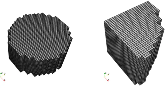
The domain Ω is discretized only on the coarse level by standard Lagrangian finite element families which satisfy the standard approximation properties. A typical reactor mesh and its x, y, z view are shown in Figure1.1. Since the reactor is symmetric along x = 0 and y = 0 planes we can divide the reactor in 4 parts and compute only one of them. In order to solve the pressure,velocity and energy fields we use the finite space of linear polynomials for Ph(Ω) and the finite space of quadratic polynomials for Vh(Ω) and Hh(Ω). The mesh is stored in the file data_in/mesh.in which is included in the program. Since the computation of such a mesh is demanding on a single machine architecture a simple example cube reactor mesh is also given to quickly test new implementations. The procedure necessary to generate the mesh.in file is the following:
1) The mesh is generated by the Gambit mesh generator (seehttp://www.fluent.com/) and stored in the file mesh.msh
2) Two mesh levels are generated by using the libmesh library and the case option of the configuration files (seehttp://libmesh.sourceforge.net/).
3) The two mesh level geometry is stored in the file data_in/mesh.in and ready to use.
Since the solver is a multigrid solver, the reactor mesh file has two mesh levels: a coarse level (level 0) and a fine level (level 1). The level 0 is the coarsest mesh necessary to describe the power and pressure loss distributions. In order to avoid the installation of the libmesh library the necessary file for the reactor is given with the program. If one wants to change the mesh is necessary to use and install the open source libmesh library and follow the above steps.
1.2.2 Reactor transfer Operators in working conditions
In order to complete the equation in section 1.1 we must define the reactor transfer operators in working conditions.
a) Incompressibility transfer operators
• Pc
ef. In the reactor model we assume incompressibility on both the coarse and the fine level and therefore
The assumption is exact since
Pefc(vbh− vh) = ∇ · ρ(bvh− vh) (1.38) is different from zero only if mass is generated at the fine level. The total mass transfer operator Pc
ef may be different from zero if there is a phase change.
b) Momentum transfer operators
• Tm
cf. It is usual to compute the term Tcfm(vh,vbh) by using the Reynolds hypothesis, namely Tcf(vh,vbh) = ∇ · ¯τbτh (1.39)
where the turbulent tensor ¯bττhis defined as ¯b
ττh = 2µτD(vbh) (1.40) with µτ the turbulent viscosity.
• Pcfm. The operator Pcf(pbh− ph,vbh − vh) defines the momentum transfer from fine to coarse level due to the sub-grid fluctuations and boundary conditions. This can be defined in a similar way by Pcf(pbh− ph,vbh− vh) = (1.41) ζ(x)³∂ ρvbh ∂t ·φbh(k) + Z Ω(∇ · ρ b vhvbh) ·φbh(k) dx − b ph∇ ·φbh(k) dx + ¯bτh: ∇φbh(k) − ρg ·φbh(k) − ∇ · ¯τbef f ´
where ζ(x) is the fraction of fuel and structural material in the total volume. The tensor ¯bτef f is defined as
¯b
τef fh = 2µef fD(vbh) . (1.42)
The values of µef f depends on the assembly geometry and can be determined only with direct simulation of the channel or sub-channel configuration or by experiment.
• Sm
cf. The operator Scfm(ph) indicates a non symmetric pressure correction from the subgrid to the pressure distributions of the assembly fuel elements. If the sub-level pressure distribution is symmetric then this term is exactly zero. Therefore we may assume in working conditions
Scfm(ph) = 0 . (1.43)
• Kcfm(vh). The operator Kcfm(vh) determines the friction energy that is dissipated at the fine level inside the assembly. We assume that the assembly is composed by a certain number of channel and that the loss of pressure in this channel can be compute with classical engineering formulas. In working conditions for forced motion in equivalent channels we may set
Kcfm(vh) = ζ(x)ρ2vbh|vbh| Deq
λ (1.44)
c) Energy transfer operators
• Te
cf. It is usual to compute the term Tcfe (Th,Tbh,vbh, vh), following Reynolds analogy for the turbulent Prandtl number Prt, as
Tcfe(Tbh, Th,vbh, vh) = ∇ · ( µt
P rt∇Tbh) (1.45) with µtthe turbulent viscosity previously defined.
• Pcfe . The operator Pcfe(vh −vbh) defines the energy exchange from fine to coarse level due to the sub-grid fluctuation and boundary conditions. This can be defined as
Pcfe(Th−Tbh) = (1.46)
ζ(x)³∂ ρ CpTbh
∂t + ∇ · (ρ CpvbhTbh) − Φh − Qh− ∇ · (k
ef f∇Tbh)´
where ζ(x) is the fraction of fuel and structural material in the volume. The values of kef f depends on the assembly geometry and can be determined with direct simulations of the channel or sub-channel configurations or by experiment.
• Se
cf. The operator Scfe (ph) is the heat source that is generated through the fuel pin surfaces. For the heat production in the core we may assume
Scfe (ph) = W0cos( πz + Hin Hout− Hin
) . (1.47)
where Hinand Houtare the heights where the heat generation starts and ends. The quantity W0
is assumed to be a known function of space which is defined by the power distribution factor (see section2.3.6)
1.2.3 Reactor Equations in working conditions
We can assume the density as a weakly dependent function of temperature and almost independent with pressure. We assume
ρ(T, P ) = ρ0(T )exp(βp) (1.48)
with β ≈ 0 and define ρin= ρ0(Tin). For this purpose it is more convenient to define a new velocity field uhsuch that
uh = vh ρ ρin
. (1.49)
For the reactor model, with vertical forced motion in working conditions, the state variables (bu,p,b T )b are the solution of the following finite element system
a) Fem incompressibility equation Z Ω ³ β ∂ph ∂t + (∇ · ρinubh) ´ b ψh(k) dx = 0 . (1.50)
b) Fem momentum equation Z Ω ∂ ρinubh ∂t ·φbh(k) dx + Z Ω(∇ · ρin b uhvbh) ·φbh(k) dx − Z Ω b ph∇ ·φbh(k) dx + Z Ω(¯ b τh+ ¯τbτh+ ¯τbef fh ) : ∇φbh(k) dx + (1.51) Z Ω 2ρinubh|vbh| Deq λ ·φbh(k) dx − Z Ω ρg · b φh(k) dx = 0 b) Fem energy equation
Z Ω ∂ ρ CpTbh ∂t ϕbh(k) dx + Z Ω ∇ · (ρinCp b uhTbh)ϕbh(k) dx − Z Ω Φhϕbh(k) dx + Z Ω(k + k ef f + µt P rt) ∇ b Th· ∇ϕbh(k) dx − (1.52) Z Ω Qh b ϕh(k) dx − Z Ω Wmaxr(x) cos ³ z + H in Hout− Hin ´ b ϕh(k) dx = 0 . for allψbh(k),φbh(k) andϕbh(k) basis functions. r(x) = 1/(1 − ζ(x)) is the coolant occupation ratio.
Equations in strong form The variational fem system (1.50-1.52) is equivalent to β∂ph ∂t + ∇ · (ρinubh) = 0 (1.53) ∂ρinubh ∂t + (∇ · ρinubhvbh) = −∇bph + ∇ · (¯τbh+ ¯τb τ h+ ¯τbef fh ) − 2ρinubh|vh| Deq λ + ρg(1.54) ∂ ρ CpTbh ∂t + ∇ · (ρinCpubhTbh) = Φh + ∇ · (k + k ef f + µt P rt ) ∇Tbh+ (1.55) Qhϕbh(k) + W0r cos³ z + Hin Hout− Hin ´ .
Boundary conditions The equations (1.53-1.55) must be completed with the corresponding boundary conditions. On the inlet surface for z = 0 we have pressure p = Pin, temperature T = Tin and no tangential component for the velocity field. On the surface x = 0 we have symmetry; the y-velocity component v is set to zero and there is no heat flux through this surface, i.e. ˙q · n = 0. In a similar way the surface y = 0 is surface of symmetry; the x-velocity component u is zero and there is no heat flux, i.e. q · n = 0. On the top we have outflow boundary conditions with pressure p = p0 = 0. On the reactor outer walls we impose totally slip boundary conditions and thermal insulation (no heat flux).
1.2.4 Thermophysical properties of liquid metals (lead)
We focused only on liquid lead as coolant. It is well known that lead-bismuth eutectic (LBE) is sometimes preferred between lead and bismuth because of its better properties like cross section, radiation damage, activation and in particular because of the fact that it has a lower melting point and it is liquid in a wider range of temperatures, which is an obvious advantage for heat removal and
safety. On the other hand, lead cooled fast reactors with nitride fuel assemblies are currently being studied in the world (e.g. BREST-300 and BREST-600) because of the lower price of the coolant. It is also to be said that, from the point of view of density and viscosity, which are our concern presently, there is no remarkable difference between lead and lead-bismuth eutectic.
Density The lead density is assumed to be a function of temperature as ρ = (11367 − 1.1944 × T )Kg
m3 (1.56)
for lead in the range 600K < T < 1700K.
Dynamic Viscosity The following correlation has been used for the viscosity µ
µ = 4.55 × 10−04e(1069/T )P a · s . (1.57)
for lead in the range 600K < T < 1500K.
Thermal Expansion For the mean coefficient of thermal expansion (AISI 316L) we assume αv = 14.77 × 10⁻⁶+ 12.20−9(T − 273.16) + 12.18−12(T − 273.16)2 m
3
K (1.58) Thermal conductivity The lead thermal conductivity κ is
κ = 15.8 + 108 × 10−4(T − 600.4) W
m · K (1.59)
Specific heat capacity at constant pressure The pressure-constant specific heat capacity for lead is assumed as not depending on temperature, with a value of
CFD Program
2.1 Introduction
2.1.1 Installation
In order to install the package, choose a directory, and run the following commands
• uncompress: tar xzvf RMCFD-1.0.tar.gz;
• go to the directory: cd RMCFD-1.0;
• run the configuration script: ./configure;
• compile the program: make ex13.
Now you are ready to run the program (see Section2.1.3). 2.1.2 Preprocessor and mesh generation
The mesh is generated by the commercial code Gambit (seehttp://www.fluent.com) and the open source libmesh library. The necessary meshes at different levels are enclosed with this package. The generation of the mesh is not argument of this report.
2.1.3 Running the code
Make. The code can be run and compiled by using the make command. The make commands are inside the file Makefile. Through the Makefile one can execute several commands
• make ex13: compile the program;
• make clean: remove the object files for the specified METHOD;
• make distclean: remove all object, executable files and dynamic libraries;
• make contrib: generate dynamic libraries needed for execution. Run the code. In order to run the program one must set in the file config.h // #define RESTART 100
#define STARTIME 0.
and execute the following commands make ex13
ex13
Restart the code. In order to restart the program from the iteration n at the time t it is necessary so set the following parameter in the config.h file
#define RESTART n #define STARTIME t and then execute
make ex13 ex13
Method. It is possible to run the code in two different ways specifying the shell parameter METHOD before the compilation. You can set this to optimized (opt) or to debug mode (dbg) using the command
export METHOD=opt
for optimized mode and similarly for debugging mode. The default mode is set to opt. 2.1.4 Postprocessing
The output is in vtk format and saved in the output directory. The open source paraview program is used. For tutorials and manuals one can see htpp://www.paraview.org and http://www.vtk.org/.
2.2 Directory structure
2.2.1 GeneralitiesThe program consists of a main directory where the source code is stored and five additional subdi-rectories. The five subdirectories are:
• config is the configuration directory where all the configuration files are stored: data.h and config.h.
• contrib is the contribution directory and stores laspack library and datagen program.
• data_in is the data directory. All the data necessary for the simulation must be stored in this directory. Enclosed with the program we have three compressed files containing the test packages. One for each test sample reported above. The tests are
– A simple hexahedral geometry (in cube.tar.gz).
– The reactor model geometry with no control rod channels (in RM1.tar.gz).
– The reactor model geometry with eight empty control rod channels (in RM2.tar.gz).
• fem is the finite element directory where the finite element Gaussian point values for integration are stored. Only the finite element Hex27, Hex8, Quad9, Quad4, Edge3 and Edge2 are in this package.
• output is the directory where the results are stored. Meshes, boundaries and field values can be found there for each time step. The data are stored in vtk format and can be read using the software paraview.
2.2.2 Main directory and C++ classes. The code is written in C++. The main file is ex13.C
which calls all the necessary functions organized in five C++ classes. The five classes are
• the class MGCase, written in the files MGCase.C and MGCase.h, defines input and output data flow;
• the class MGGauss, written in the files MGGauss.C and MGGauss.h, defines Gaussian integration;
• the class MGMesh, written in the files MGMesh.C and MGMesh.h, defines the geometrical mesh;
• the class MGSol, written in the files MGSolver.C MGSolver3DNS.C and MGSolver.h, defines the Navier-Stokes equation solver;
• the class MGSolT, written in the files MGSolverT.C MGSolver3DT.C and MGSolverT.h, defines the energy equation solver.
Here are the classes, structs, unions and interfaces with brief descriptions:
MGCase(Class for generation of the case data for computation ) . . . 50
MGGauss(Class that contains the Gaussian points for standard fem ) . . . 52
MGMesh(Class for MG mesh ) . . . 53
MGSol(Class for MG Navier-Stokes equation solvers ) . . . 55
MGSolT(Class for MG Energy equation solvers ) . . . 58
2.2.3 Directory config
This directory consists of two configuration files
• config.h with the configuration variables (solution of Navier-Stokes system, solution of en-ergy system, boundary integration, etc ...)
• data.h with constant material properties and numerical parameters. 2.2.4 Directory contrib
In this directory you can find two packages
• laspack is a linear algebra library for solving large sparse linear systems. For details see http://www.mgnet.org/mgnet/Codes/laspack/html/laspack.html.
• datagen contains the program that generates the desired volumetric power and pressure loss distribution. For datails see Section2.3.6.
2.2.5 Directory data_in
The partial differential equations governing the system must be discretized in matrices and vectors. The structures of these matrices and vectors are stored in files in the directory data_in. Each geometry required a new set of files. The libmesh library is needed for this generation.
All the necessary files are contained in data_in/packagename.tar.gz. In order to expand the compressed file one must set the cursor in the directory data_in and then use the command tar xvf packagename.tar.gz. In this directory you should find the following files
• mesh.in. The mesh file
• matrix0.in. The Navier-Stokes matrix file at level 0
• matrix1.in. The Navier-Stokes matrix file at level 1
• matrixT0.in. The energy matrix file at level 0
• matrixT1.in. The energy matrix file at level 1
• prolT1.in. The prolongation operator for energy equation
• rest0.in. The restrictor operator for Navier-Stokes equations
• restT0.in. The restrictor operator for energy equation
• data.in. The data power and loss pressure factor file (level 1)
If the data.in is not in this directory it will be generated from the program (with all 1). 2.2.6 Directory fem
This directory consists of six files with Gaussian integration point values
• shape1D_0302.in with 1-dim Gaussian points for integration of a fem Edge2 linear element
• shape1D_0302.in with 1-dim Gaussian points for integration of a fem Edge3 linear element
• shape2D_0904.in with 2-dim Gaussian points for integration of a fem Quad4 linear ele-ment
• shape2D_0909.in with 2-dim Gaussian points for integration of a fem Quad9 quadratic element
• shape3D_2708.in with 3-dim Gaussian points for integration of a fem Hex8 linear element
• shape3D_2727.in with 3-dim Gaussian points for integration of a fem Hex27 quadratic element
2.2.7 Directory output
This is the directory where the results are printed. In order to analyze the data with paraview viewer you can open different file
• mesh.0.vtu contains only the 3D geometric mesh. It is used to check the input geometry.
• boundary.0.vtu contains the boundary geometry. With this file you can visualize and check boundary conditions.
• Out.n.vtu contains the pressure, temperature and velocity solution at the time step n.
• time.pvd contains the xml list of all time steps. If you load this file inside paraview you can visualize the time sequence of the solution.
2.3 Configuration, data and parameter setting
Enclosed with the program there are three sample outputs. One for each test reported here. The tests are as follows
• a) cube.tar.gz a simple lightweight hexahedral reactor for quick testing.
• b) rm1.tar.gz a test reactor without the rod control channel, i.e. the rod control channel is assumed to be full of coolant.
• c) rm2.tar.gz a test reactor with eight empty rod control channels. In order to run a total new computation the following steps are necessary
• Untar the archive in the directory data_in (tar xzvf packagename.tar.gz)
• Set the configuration file data_in/config.h
• Set the physical properties in data_in/data.h
• Set the boundary conditions in the files MGSolver3DNS.C and MGSolver3DT.C
• Set the additional reactor parameters at the top of the files MGSolver3DNS.C and MGSolver3DT.C
Standard configuration for the mentioned tests is provided with the packages. 2.3.1 Configuration
The configuration file is config/config.h. An example of configuration file can be found in
A.3. Options are set via define (#define command in C or C++). The option is not active when the corresponding define is commented. For example if one sees in the file config/config.h a define as
# define NS_EQUATIONS 1
then the Navier Stokes solver is active. If the define option is with a comment (// is the comment operator in C++) as
// # define NS_EQUATIONS 1
then the Navier Stokes solver is not active and the Navier Stokes will not be solved. The number after the define is necessary and sometimes such a number is used in the program for further options. Many of the options in the file config/config.h are not important for our problems. They remain in the configuration file for compatibility with the CFD multipurpose code. The following options, shown in Table2.3.1, are important for this code:
• DIM2. With this option you need to set the dimensions of the problem as in Table2.3.1. For RM reactor and test cube reactor use always 3D option, so the 2D option should be eliminated, i.e.
help command option description 3D active //#define DIM2 1 3D simulation Bound. integr. active //#define BOUNDARY 1 Boundary integration NS equation active #define NS_EQUATIONS 1 Solve the Navier-Stokes eqs Energy equation active #define T_EQUATIONS 1 Solve the Energy eqs Restart time #define RESTARTIME 1.1 Initial time set to t = 1.1 Restart active #define RESTART 10 Restart from file label 10 Case active #define GENCASE 1 Generate the case files libemesh active #define LIBMESHF 1 linking with libMesh lib GMV graphics active #define OUTGMV 1 output with GMV Print step #define PRINT_STEP 10 Print each 10 steps
Info active #define PRINT_INFO 1 Print info after function execution LX dimension #define LX 2. Set the x-dimension LX =2 LY dimension #define LY 2. Set the y-dimension LY =2 LZ dimension #define LZ 2. Set the z-dimension LZ =2
Table 2.1: Options in config.h file
• BOUNDARY. The boundary option is necessary for integration on boundary. Since we have a pressure condition on the boundary (reactor bottom and top) this option is necessary, i.e. # define BOUNDARY 1
• NS_EQUATIONS, T_EQUATIONS. If the system has the (p, u) state then you must solve only the Navier-Stokes equations. If the system has the (p, u, T ) state then you must solve the Navier-Stokes equation and the energy equation. For RM reactor we must set
# define NS_EQUATIONS 1 # define T_EQUATIONS 1
• RESTARTIME, RESTART. In order to restart your program from the solution at t = 1.1 written in the file Out.10.vtu one must set the restart option and the restart time, i.e. #define RESTARTIME 1.1
#define RESTART 10 .
In order to start from zero (t = 0.) with initial conditions as in section2.3.4one must set #define RESTARTIME 0.
// #define RESTART 10 .
• GENCASE, LIBMESHF. In order to avoid the installation of the libMesh library all the necessary files are given to you. In this case you must set
// #define GENCASE 1 // #define LIBMESHF 1 .
In order to generate a new geometry and therefore a new case of files one must set #define GENCASE 1
#define LIBMESHF 1 .
For this option you must install the libmesh library. See http://libmesh.sourceforge.net/for details.
• GMV. This set all the output file in the GMV format (see http://laws.lanl.gov/XCM/gmv/GMVHome.html). This is not the case for
this version where all the output files are in vtk format. Data analysis is carried out by Paraview (seehttp://www.paraview.org/). We set
// #define GMV 1
• PRINT_STEP. With this option the program prints every PRINT_STEP iterations. You must edit this option to print every 10 step as
#define PRINT_STEP 10
• PRINT_INFO. With this option the program prints a message from each routine. It is useful for debugging. Let set
#define PRINT_INFO 1
for printing only messages from routines and set // #define PRINT_STEP 1
during optimized execution.
• LX, LY, LZ. These are parameters useful for defining the dimensions of the reactor. In this program they are used only in setting the boundary conditions. The geometry is not affected by this parameters if the geometry is read from an external file. In our case the geometry is read from the file mesh.in. We set
#define LX 2. #define LY 2. #define LZ 2.
in order to have LZ= 2m as a reference length of the reactor (see section2.3.3) 2.3.2 Data
The configuration file is config/data.h. An example of data file can be found in sectionA.3.3. The data values are defined by using the define command (#define command in C or C++). For example if we see in the file config/data.h a define as
# define RHO0 10000
then the density RHO0 takes the value of 10000. The units are always in agreement with the interna-tional system.
The parameters to set from this file are as follows:
• ND_TIME_STEP ,TIME,N_TIME_STEPS. This values are the values of the time step, the initial time and the number of time steps. In order to start at t = 0 and perform 100 time steps of length ∆t = 0.01 one must set
#define ND_TIME_STEP 0.01 #define TIME 0.0
#define N_TIME_STEPS 100 .
• Uref,Lref,T_ref,RHOref. These are the reference values of velocity, length, tempera-ture and density. The pressure reference is RHOref Uref Uref. We set T_ref= 1000 in order to have a temperature in kK (kilo Kelvin) and RHOref= 100000 in order to have the pressure in 0.1M P a. All these for graphical purpose in Paraview. Therefore in this case one sets
command option description #define Uref 1. Reference velocity #define Lref 1. Reference length #define T_ref 1000. Reference temperature #define RHOref 100000. Reference density #define T_IN 673.15 Inlet temperature #define P_IN 36000. Inlet pressure #define RHO0 11367.0 density at T∗1
#define MU0 .0022 viscosity at T∗2
#define KAPPA0 15.8 conductibility at T∗3
#define BP0 147.3 conductibility at T∗4
#define KOMP0 0. compressibility at T∗5
#define ND_TIME_STEP 0.05 Time step ∆t #define TIME 0.0 Initial time t #define N_TIME_STEPS 100 Number of time steps #define QHEAT 1.15e+8 heat volume density source #define DIRGX 0. gravity x-direction #define DIRGY 0. gravity y-direction #define DIRGZ 0. gravity z-direction
Table 2.2: Parameters in data.h file
command value description
#define ILUINIT 100 ILU decomposition each 100 steps
grid0 0 bottom grid level
gridn 1 top grid level
MaxIter 15 Iteration multigrid (max)
Eps 1.e-6 residual accuracy
MLSolverId MGIterId Multigrid type
Gamma 2 Multigrid cycle (1=V cycle 2=W Cycle)
RestrType 1 restriction operator(1. simple 2. weighted)
Nu1 8 Number of pre-smoothing iterations
Nu2 8 Number of post-smoothing iterations
Omega 0.98 Relaxation parameter for smoothing
SmoothProc GMRESIter Smoothing method
PrecondProc ILUPrecond Preconditioner
NuC 40 Number of iterations on coarsest grid
OmegaC 0.98 Relaxation parameter on coarsest grid SolvProc GMRESIter Coarsest level Iterative method PrecondProcC (PrecondProcType)NULL Coarsest level preconditioner
Table 2.3: Parameters for multigrid in data.h file
#define Uref 1. #define Lref 1. #define T_ref 1000.
#define RHOref 100000.
• T_IN, P_IN. This are the temperature and the pressure at the inlet of the reactor. If we want a a loss of pressure across the reactor of 36000P a and a temperature of 673.15K one must set #define T_IN 673.15
#define P_IN 36000.
• RHO0,MU0, KAPPA0, CP0. The value RHO0 of the lead density at temperature T∗1 = 0K is set to 11367, the value MU0 of the lead viscosity to 0.0022, the value KAPPA0 of the conductibility at temperature T∗3 = 673.15K to 15.8 and the value CP0 of the pressure specific heat to 147.3. In our case we set
#define RHO0 11367.0 #define MU0 .0022 #define KAPPA0 15.8 #define CP0 147.3.
The temperature dependence is set inside the single files: MGSol3DT.C (energy equation) and MGSol3DNS.C (Navier-Stokes system). For details see section2.3.5.
• QHEAT. The average volumetric heat source for the reactor is set by this parameter as #define QHEAT 1.15e+8.
The sinusoidal shape and other source factors are set directly inside the file MGSol3DT.C. The power factor distribution of the assemblies is in the file data.in in the directory data_in. See section2.3.6.
• DIRGX, DIRGY, DIRGZ. Gravity can be set by using these parameters. If one wants grav-ity (ρg) along the z-axis one must set
#define DIRGX 0. #define DIRGY 0. #define DIRGZ 1.
All the value are in g = 9.81m/s2units.
Among the solution methods one can choose one of these methods 1. Jacobi = JacobiIter
2. SOR forward = SORForwIter 3. SOR backward = SORBackwIter 4. SOR symmetric = SSORIter 5. Chebyshev = ChebyshevIter 6. CG = CGIter 7. CGN = CGNIter 8. GMRES(10) = GMRESIte 9. BiCG = BiCGIter 10. QMR = QMRIter 11. CGS = CGSIter 12. Bi-CGSTAB = BiCGSTABIter 13. Test = TestIter .
Among the preconditioner matrices we can have 0. none = (PrecondProcType)NULL
1. Jacobi = JacobiPrecond 2. SSOR = SSORPrecond 3. ILU/ICH = ILUPrecond.
Standard configuration uses GMRES and ILU preconditioner and the values shown in Table2.3.2. 2.3.3 Boundary conditions
The boundary conditions are already set for the reactor. In order to change the boundary conditions, it is necessary to edit the user part in the appropriate function. For pressure and velocity boundary con-ditions one must edit the function void MGSol::GenBc(const unsigned int Level) in the file MGSolver3DNS.C. If you open the mentioned file you can find
/// Here is the space for user code contribution // ********************************************* // boundary conditions box
if (zp < 0.001) { // top side (inlet) bc[Level][dof_u]=0; bc[Level][dof_v]=0; // inlet pressure p=p_in
if (i<n_p_dofs) bc[Level][idx_dof[k+3*n_nodes]]=0; }
if (zp > LZ-0.001) {// bottom side (outlet) bc[Level][dof_u]=0; bc[Level][dof_v]=0; // outlet pressure p=0 } //symmetry if (xp < 0.001) { // side 1 bc[Level][dof_u]=0; } if (xp > LX-0.001) { // side 3 bc[Level][dof_u]=0; } if (yp < 0.001) { // side2 bc[Level][dof_v]=0; bc[Level][dof_u]=0; }
if (yp > LY-0.001) { // side4
bc[Level][dof_v]=0; bc[Level][dof_u]=0; }
// **************************************
The vertex point (xp, yp, zp) can be used to set all the necessary boundary conditions. The face middle point is also provided as (xm, ym, zm).
For boundary conditions of the energy equation one must edit the function void MGSol::GenBc(const unsigned int Level) in the file MGSolver3DT.C. If you open the mentioned file you may find
// ******************************************** // boundary conditions on a reactor
if (zp < 0.001) bc[Level][dof_u]=0;
// ******************************************** The same points are provided also for this equation.
2.3.4 Initial conditions
Initial pressure velocity solution. If one wants to set the initial solution in pressure and velocity it is necessary to edit the function void MGSol::GenSol(const unsigned int Level) inside the file MGSolver3DNS.C. If you open the mentioned file you may find the initial solution u = 0 and p which changes linearly from P_IN to zero over the z-axis. Therefore in the appropriate part of the function you have
// *************************
/// Here is the space for user contribution u_value =0.;
w_value =0.;
p_value=(P_IN/(RHOref*Uref*Uref))*(LZ-zp)/LZ; u_value=0.;
// ************************
Initial Energy solution. If one wants to set the initial solution in temperature one must edit the function void MGSolT::GenSol(const unsigned int Level) inside the file MGSolver3DT.C. If you open the mentioned file you can find a constant initial solution T=T_IN/Tref over all the domain. The inlet temperature T=T_IN and the reference temper-ature T=Tref, are defined in the file config/data.h. The reference tempertemper-ature is actually T ref = 1000 in order to have temperature values in the range 0 − 1kK (mainly for graphical pur-poses). In the user area of the file MGSolver3DT.C you will find
// *************************
/// Here is the space for user contribution u_value =T_IN/Tref
// *************************
2.3.5 Physical property dependence on temperature
The code can run with lead properties that can be considered as a function of temperature. These functions are defined directly in the files where they are used. If the property law must be modified is necessary to change the inline functions at the top of the followings:
- MGSolver3DNS.C for the momentum equations; here are defined ρ = ρ(T ) and ν = ν(T ) - MGSolver3DT.C for the energy equation; here are defined ρ = ρ(T ), κ = κ(T ) and Cp= Cp(T ). Furthermore, you have to set #define RT 1 in config/data.h in order to switch on tempera-ture dependence.
2.3.6 Power distribution and pressure loss distribution
The power distribution and the pressure loss distribution are set in the file data_in/data.in. The file looks like this
Level 0 64 0 0.375 0.375 0.375 1.03 1 1 0.875 0.375 0.375 0.91 1 2 1.375 0.375 0.375 1.02 1 3 1.875 0.375 0.375 1.12 1 4 0.375 0.875 0.375 1.04 1 5 0.875 0.875 0.375 0.78 1 6 1.375 0.875 0.375 1.02 1 7 1.875 0.875 0.375 1.1 1 ... ...
The file shows for each element: the element number, the x-coordinate, the y-coordinate, the z-coordinate, the value of the power distribution factor and the value of the pressure loss factor. The file can be generated by a program that is enclosed in the directory contrib/datagen. The direct editing is not very easy since there are at the level 1 more than 15000 elements. The file should be completed at all mesh levels. The procedure to have a new power distribution is as follows:
• delete the file data_in/data.in
• run the code with no data_in/data.in file. Then a new data_in/data.in is generated and the code stops.
• edit the values of power distribution or
• copy the file data_in/data.in in contrib/datagen/data.orig
• edit contrib/datagen/datagen.H inserting power distribution factors as in Figure3.3. Power distribution from Figure3.3is set as follows
#define A1_1 1.05 #define A1_2 1.03 #define A1_3 1.02 #define A1_4 1.02 #define A1_5 1.04 #define A1_6 1.17 #define A1_7 1.12 #define A2_1 1.05 #define A2_2 1.03 #define A2_3 1.02 #define A2_4 1.02 #define A2_5 1.12
#define A2_6 1.12 #define A2_7 1.03 #define A2_8 0.81 #define A3_1 1.04 #define A3_2 1.04 #define A3_3 1.02 #define A3_4 1.10
#define A3_5 CONTROL_ROD #define A3_6 0.96 #define A3_7 0.87 #define A4_1 1.04 #define A4_2 1.03 #define A4_3 1.03 #define A4_4 1.04 #define A4_5 1.10 #define A4_6 0.97 #define A4_7 0.86 #define A5_1 1.02 #define A5_2 1.11 #define A5_3 1.10 #define A5_4 1.15 #define A5_5 1.01 #define A5_6 0.85 #define A6_1 1. #define A6_2 1.06
#define A6_3 CONTROL_ROD #define A6_4 0.99 #define A6_5 1.07 #define A6_6 0.78 #define A7_1 1.04 #define A7_2 0.95 #define A7_3 0.98 #define A7_4 0.81 #define A8_1 0.94 #define A8_2 0.89 #define A8_3 0.74
The power distribution in Figure3.3is enclosed with the provided package. The pressure loss distri-bution enclosed in the code is constant and equal to 1.
Tests
3.1 Monodimensional test (test1)
3.1.1 Monodimensional equationsIn steady working conditions with constant properties (see Table3.1.2) and velocity in the z-direction the (1.50-1.52) becomes a) Incompressibility constraint ∂wbh ∂z = 0 (3.1) b) Momentum equation ∂pbh ∂z = 2ρwb2 Deq λ (3.2) b) Energy equation ρ Cpwbh ∂Tbh ∂z = κ ∂2Tbh ∂z2 + ˙q 000 r . (3.3)
These equations can be solved and therefore the solution can be used to test the code in this trivial case.
3.1.2 Monodimensional analytic test
The problem (3.1-3.3) can be further simplified for some velocity ranges for which the thermal con-ductivity κ can be neglected. If we assume κ = 0 the system, after integration along the z-axis, yields b wh = const (3.4) b pin−pbout = 2ρwb2 Deq λ(wbh) H (3.5) ρ Cpwbh(Tbout−Tbin) = ˙Q r (Hout− Hin) , (3.6)
properties value ρ (11367 − 1.1944 × 673.15) = 10562 µ 0.0022 Deq 0.0129 κ 15.8 + 108 × 10−4(673.15 − 600.4) = 16.58 Cp 147.3 r 0.545 Table 3.1: Properties at T=673.15K
where H is the total height of the reactor, Hin and Hout are the starting and ending point of the heat generation. In order to compute (wh, ph, Th) we set each property to be constant (see Table3.1.2). Velocity. The velocity must be solved iteratively. At the step 0 we guess the solution as w = 1.51m/s. Then the Reynolds number gives
Re = ρ w Deq
µ = 10562 × 1.51 × 0.0129/0.0022 = 93526 (3.7) and the friction coefficient yields
λ = 0.079
Re0.25 = 0.004517 . (3.8)
The velocity is then w = s 2 PIN Deq ρ 4 ∗ λLZ = s 2 36000 × 0.0129 10562 ∗ 4 ∗ 0.0045174 × 2. = 1.5598 . (3.9) Iteratively we find w = 1.567m/s. Each step is recorded in Table3.2.
step guess w Re λ w
1 1.5100 93525 0.004517 1.559 2 1.559 96611 0.004481 1.566 3 1.566 97004 0.004476 1.567 4 1.567 97053 0.004476 1.567 Table 3.2: Iterative velocity computation.
Temperature. The temperature can be computed as Tout− Tin= ˙ Q r ˙m cP(Hout− Hin) = 1.14591 × 10⁸ 0.548 × 1.567 × 147.3 = 85.76K At the top of the reactor we obtain a constant temperature distribution with value
Figure 3.1: Test1: Full reactor and computational domain.
3.1.3 Simulations with constant axial power distribution (test1)
With constant power distribution along the z-axis we obtain a value of velocity in full agreement with (3.1.2). The geometry is shown in Figure3.1and packaged in data_in/cube.tar.gz. The main options for the config/config.h file are
#define BOUNDARY 1 #define NS_EQUATIONS 1 #define T_EQUATIONS 1 #define RESTARTIME 0. #define PRINT_STEP 2
The data are set as following ( config/data.h) // time #define ND_TIME_STEP 0.01 #define TIME 0.0 #define N_TIME_STEPS 500 // Reference quantities #define Uref 1. #define Lref 1. #define Tref 1000. #define RHOref 100000. // Inlet #define P_IN 36000. #define T_IN 673.15
// fluid properties #define RHO0 11367.0 #define MU0 .0022 #define NUT .0 #define KAPPA0 15.8 #define CP0 147.3 // Heat source
#define QHEAT 1.14591e+8 // temperature function #define RT 0. // Gravity #define DIRGX 0. #define DIRGY 0. #define DIRGZ 0.
The parameter RT is set to 0, meaning that physical properties do not depend on temperature. The boundary conditions in MGSolver3DNS.C are
// boundary conditions box
if (xm < 0.001) { // y-z symmetry plane bc[Level][dof_u]=0;
}
if (ym < 0.001) { // x-z symmetry plane bc[Level][dof_v]=0;
}
if (xm > 0.001 && ym > 0.001 &&
zm < LZ-0.001 && zm > 0.001) { // reactor boundary bc[Level][dof_u]=0; bc[Level][dof_v]=0; } if (zm > LZ-0.001 ) { // top } if (zm < 0.001) { // bottom bc[Level][dof_u]=0; bc[Level][dof_v]=0; if (i<n_p_dofs) bc[Level][idx_dof[k+3*n_nodes]]=0; }
The planes x = 0 and y = 0 are symmetry planes. On the reactor boundary we set no tangential and not-crossing conditions. On the bottom, we impose inlet pressure P_IN equals to 36000 and velocity parallel to z-axis. On the top we set free outflow boundary conditions.
The boundary conditions in the file MGSolver3DT.C are as follows // boundary conditions on a box
The only condition imposed is at the inlet: the temperature is fixed at the T_IN equal 673.15 value. No heat flux condition is set over the remaining boundary. As expected the velocity profile is monodi-mensional. The w-component is constant along the channel and reaches the expected analytic solution value of 1.567m/sec. In the initial part of the reactor ( 0 < z ≤ Hin), where no source generation is present, the temperature is constant (T = Tin = 673.15K). Then, it assumes a linear profile in consequence of constant power generation ( Hin < z < Hout). In the upper part of the reactor ( Hout≤ z < H) the profile is again constant. The value of temperature on the top is 758.9K.
3.2 Simulations of a test reactor model
3.2.1 Reactor model coreFigure 3.2: Scheme of a quarter of the Reactor model.
For the reactor model we consider the rector in Figure3.2where only a quarter of the total geometry is reported. The fuel assembly consists of n × n pins lattice resulting in 170 positions fitting the required core area in a circular arrangement. The model design distributes the fuel assemblies in three zones: 56 fuel assemblies in the inner zone, 62 fuel assemblies in the intermediate zone and the remaining 44 fuel assemblies in the outer one. The power distribution factors, i.e. the power of a fuel assembly
upon the average fuel assembly power, are mapped in Figure3.3. The maximum peak factor is 1.17, while the minimum is 0.74.
Figure 3.3: Reactor model power distribution.
We label the assemblies as in Figure3.2; the first row is labeled A1_i for i= 1, . . . , 8, the second row A2_i for i= 1, . . . , 7 and so on. We remark that the fuel assembly configuration is not based on a Cartesian grid but rather over a staggered grid. The length of a square assembly (LFA) is 0.294m in working conditions at the temperature of 673.15K. The reactor is cooled by lead which enters at the temperature of 673.15K. We are interested only in core active part and therefore in our computational description we consider a region which is 0.9m below the core and 0.2m above the core for a total of 2m. The heat generation zone or the active core zone for the reactor starts at Hin = 0.9m and ends at Hout = 1.8m. The reactor is cooled by lead which enters at the temperature of 673.15K. Since our model describes the reactor at assembly level the sub-assembly composition is seen as an homogeneous medium. Data about this model composition are assumed as Table3.3. In particular we
area (m2)
Pin area 370.606 × 10⁻⁴
Corner box area 5.717 × 10⁻⁴
Central box beam 2.092 × 10⁻⁴ Channel central box beam area 12.340 × 10⁻⁴
Coolant area 473.605 × 10⁻⁴
Assembly area 864.360 × 10⁻⁴
Coolant/Assembly ratio 0.548 Table 3.3: Coolant assembly area ratio data
3.2.2 Test without control rod assemblies (test2)
Figure 3.4: Test2. Full reactor and computational domain.
This test is a monodimensional simulation of the model reactor. No turbulent coefficients, no rod control assemblies and no pressure loss and power distribution factors are taken into account. In the above conditions, the solution may be considered monodimensional and therefore the results of the previous section must be recovered. The geometry is shown in Figure3.4 and packaged in data_in/RM.tar.gz. Each assembly is represented by 4 × 10 Hex27 finite elements. Since the reactor is symmetric along x = 0 and y = 0 planes we can divide the reactor in 4 parts and compute only one of them, as shown in Figure3.4. For this quarter of the reactor the nodes are 116481, the dofs 481485 (velocity, pressure and temperature) and the elements are 15561. In order to expand the compressed file one must reach the directory data_in and then type the command
tar xvf RM.tar.gz.
The main options for the config/config.h file are #define BOUNDARY 1
#define NS_EQUATIONS 1 #define T_EQUATIONS 1 #define RESTARTIME 0. #define PRINT_STEP 2
The data are set as following ( config/data.h) // time
#define ND_TIME_STEP 0.01
#define TIME 0.0
#define N_TIME_STEPS 500 // Reference quantities
#define Uref 1. #define Lref 1. #define Tref 1000. #define RHOref 100000. // Inlet #define P_IN 36000. #define T_IN 673.15 // fluid properties #define RHO0 11367.0 #define MU0 .0022 #define NUT .0 #define KAPPA0 15.8 #define PRT 0.9 #define CP0 147.3 // Heat source
#define QHEAT 1.14591e+8 // temperature function #define RT 0. // Gravity #define DIRGX 0. #define DIRGY 0. #define DIRGZ 0.
The parameter RT is set to 0, meaning that physical properties do not depend on temperature. It is necessary to keep a small time step ND_TIME_STEP in order to assure convergence. The value ∆t = 0.01 may be sufficient. The boundary conditions in the file MGSolver3DNS.C are
// boundary conditions box
if (xm < 0.001) { // y-z symmetry plane bc[Level][dof_u]=0;
}
if (ym < 0.001) { // x-z smmetry plane bc[Level][dof_v]=0;
}
if (xm > 0.001 && ym > 0.001 &&
zm < LZ-0.001 && zm > 0.001) { // reactor boundary bc[Level][dof_u]=0; bc[Level][dof_v]=0; } if (zm > LZ-0.001 ) { // top } if (zm < 0.001) { // bottom bc[Level][dof_u]=0; bc[Level][dof_v]=0;
if (i<n_p_dofs) bc[Level][idx_dof[k+3*n_nodes]]=0; }
As usual, the planes x = 0 and y = 0 are symmetry planes. On the reactor boundary we set no tangential and not-crossing conditions. On the bottom, we impose inlet pressure P_IN equals to 36000 and velocity parallel to z-axis. On the top we set free outflow boundary conditions.
The boundary conditions in MGSolver3DT.C are as follows // boundary conditions on a box
if (zp < 0.001) bc[Level][dof_u]=0;
The only condition imposed is at the inlet: the temperature is fixed at the T_IN equal 673.15 value. No heat flux condition is set over the remaining boundary.
Figure 3.5: Test2. Paraview screen shot.
We assume constant properties as in Table3.1.2and introduce sinusoidal power generation along the z-axis in the form
˙q000 = W0 π(Hout2− Hin)sin
³ πz
(Hout− Hin) ´
(3.10)
with W0 constant over all the domain Ω. This implementation guarantees that the total power
gen-erated remains the same as the other tests. A paraview snapshot of the solution is in Figure3.5. The pressure, shown in Figure reffigtest2par, is linear and matches exactly the analytical solution. As expected, the velocity profile, shown in Figure3.6, is monodimensional and constant with value 1.567m/sec. The temperature, shown in Figure 3.6, is constant for the initial part of the reactor where no source generation is present then assumes the standard profile with sinusoidal heat source and finally is constant again on the top of the reactor. The value of temperature is again 758.89K.
0 0.5 1 1.5 2 z (m) 0 0.05 0.1 0.15 0.2 0.25 0.3 0.35 0.4 p (bar) 0 0.2 0.4 0.6 0.8 1 1.2 1.4 1.6 1.8 2 z (m) 1.5 1.51 1.52 1.53 1.54 1.55 1.56 1.57 1.58 1.59 1.6 v (m/s) 0 0.2 0.4 0.6 0.8 1 1.2 1.4 1.6 1.8 2 z (m) 0.62 0.64 0.66 0.68 0.7 0.72 0.74 0.76 0.78 0.8 T (kK)
Figure 3.6: Test2. Velocity and pressure distribution (top) and temperature profile along the z-axis (bottom).